At a glance
The paper extends affine repulsive control buffers to hybrid systems whose state can jump at known guards. A nonlinear actor handles the task away from constraints, while two affine actors intervene before continuous boundary crossings and unsafe resets. Finite vertex checks can establish first-order invariance when a valid uniform dynamics-approximation bound and suitable buffer geometry are available. Two simulated systems report 100/100 safe task completions. The higher-relative-degree argument and several experimental definitions contain unresolved inconsistencies, so those results should be distinguished from a fully verified general safety certificate.
I INTRODUCTION
Continuous motion can be made repulsive near a state constraint, yet an impact can still jump directly into an unsafe state. Extending POLICEd-RL and its high-relative-degree variant, the proposal therefore adds a second buffer before states whose known reset would violate the original constraint. Both buffers use affine policies; a separate nonlinear policy retains task expressivity elsewhere.
The contribution is a conditional control construction and a switched training architecture, demonstrated on a pendulum that catches a pin and a paddle that hits a ball. “Black-box” refers to continuous dynamics available through evaluation; guards and affine reset maps are assumed known. This edition covers the complete 11-page v2, dated 26 September 2026, retaining all seven figures, the results table, 28 numbered equations, an additional unnumbered buffer display, and 41 references.
II Related Work
II-A Safety for Hybrid Systems
Control barrier functions, hybrid barrier certificates and reachability methods describe conditions for remaining in a safe set. Hybrid variants must account for both flows and resets. This work emphasizes learning without an analytical continuous-dynamics formula, but still requires simulator evaluations, known transition structure and a reliable local approximation-error bound. Its distinction is not absence of all model information.
The related-work discussion contrasts model-dependent methods with learned certificates and hybrid reachability. These citations position the method; the two numerical comparisons do not demonstrate that every alternative lacks guarantees or scales worse.
II-B Constraints in Reinforcement Learning
Expected-cost constraints in constrained MDPs and algorithms such as CPO differ from enforcing a state inequality at every time. Learned barriers, safe policy updates and model-predictive safety filters offer other tradeoffs among model assumptions, uncertainty and runtime optimization. The present analysis is deterministic apart from initial-state sampling and targets a deployment property after verification, not safe exploration throughout training.
III Problem Formulation
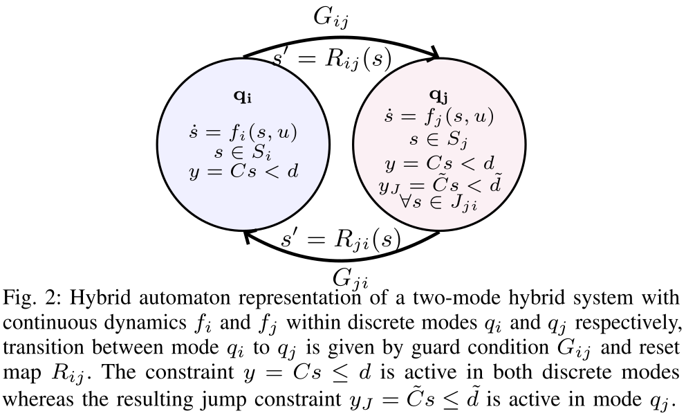
The hybrid automaton has finitely many modes, a continuous state and control, mode-specific evaluable dynamics, initial-state distribution, transition relation, guards and resets. A guard triggers a forced transition; a known affine map gives the post-reset state. The target is a known scalar affine inequality Cs≤d, initially of relative degree one, while a deterministic policy maximizes discounted reward.
Relative degree counts differentiations before control appears. A reset can turn the original constraint into a different pre-impact constraint, potentially requiring a higher-order construction. The policy must start from an admissible state and respect the relevant bounds and transition assumptions. Estimating guards or reset maps from data, as the paper suggests, would introduce uncertainty that is not covered by the exact-known-map theorem.
The infinite-horizon objective is formal; experiments use finite rollouts. The text allows discount one without specifying conditions for a finite return. Mode-dependent constraints in the pendulum example also require more bookkeeping than the initial mode-independent scalar presentation.
Equation 1
| (1) |
Original selectable caption
Equations 2–5
| (2) |
| (3) |
| (4) |
| (5) |
IV Our Framework
The design separates three questions: prevent continuous escape from the safe set; avoid guard states with unsafe reset images; and train a policy that meets the required inequalities. A learned affine architecture makes finite checks possible, but architecture and reward penalties alone do not establish the inequalities or the required uniform approximation bound.
IV-A Safety in a Discrete Mode
A strip of width w immediately below Cs=d forms the continuous-flow buffer. It must be a bounded convex polytope with known vertices, and the sampled implementation must not skip across it between decisions. Within the buffer the policy is affine. An auxiliary affine dynamics fit need not be supplied to the policy, but its projected error must be bounded by ε for every state in the buffer and every admissible action.
Theorem 1 requires Cf(v,π(v))≤−2ε at each vertex. One ε absorbs the discrepancy between actual and affine dynamics at the vertices. Affineness of the policy and approximation then interpolates the margin to every convex combination, and the second ε covers actual dynamics in the interior. Thus the output derivative is nonpositive throughout the buffer, preventing a continuous trajectory from crossing the constraint boundary under the stated assumptions.
The proof is a useful conditional certificate. A least-squares residual on sampled state–action pairs is not automatically a uniform error bound on their continuum. Convexity and boundedness of the mode domain are also needed; intersection with an arbitrary mode set need not yield the claimed polytope. The source alternates a strict safe set Cs<d with a non-strict target Cs≤d; the hard constraint being assessed is the latter.
Equations 6–11
| (6) |
| (7) |
| (8) |
| (9) | ||||
| (10) | ||||
| (11) | ||||
IV-B Safety When Transitioning Between Modes
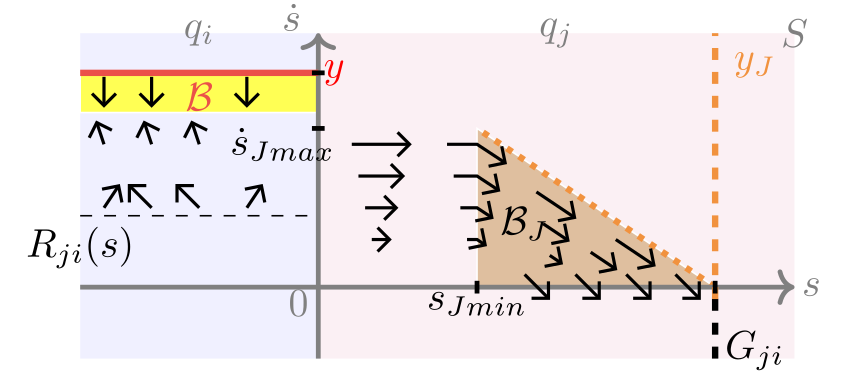
The unsafe portion of a guard consists of states with C R(s)>d. For R(s)=Ms+p, the reset condition becomes (CM)s≤d−Cp before impact. If this transformed output has relative degree one, Lemma 1 applies the same vertex certificate in a second buffer and keeps the trajectory from entering the unsafe guard. The buffer must protect the approach to the guard, not merely impose an inequality on states already defined as violating it.
For relative degree two, the proposed triangular buffer allows positive approach velocity away from the boundary, while requiring it to fall to zero at the boundary. Its slope β is the maximum entry velocity divided by the available output-distance margin. The intended interior condition is output acceleration no greater than −β times output velocity. With an admissible entry condition, this can keep the trajectory within a braking envelope.
Theorem 2’s general derivation needs qualification. It mixes scalar output derivatives with vector state derivatives and interpolates state derivatives as though they were affine, although the continuous dynamics may be nonlinear. Affine control actions alone do not justify that step. The appendix also overstates what follows from the differential inequality. The full original proof is retained; the first-order argument and reported simulations do not independently repair this higher-order gap.
The corollary combines valid flow and reset conditions across every relevant mode and transition. Multiple constraints would require compatible actors and buffers, including overlap and switching rules; simply adding actors does not establish their joint feasibility. These extensions are proposed rather than evaluated on a general high-dimensional hybrid system.
Equations 12–14
| (12) |
| (13) |
| (14) |
IV-C Training Pipeline
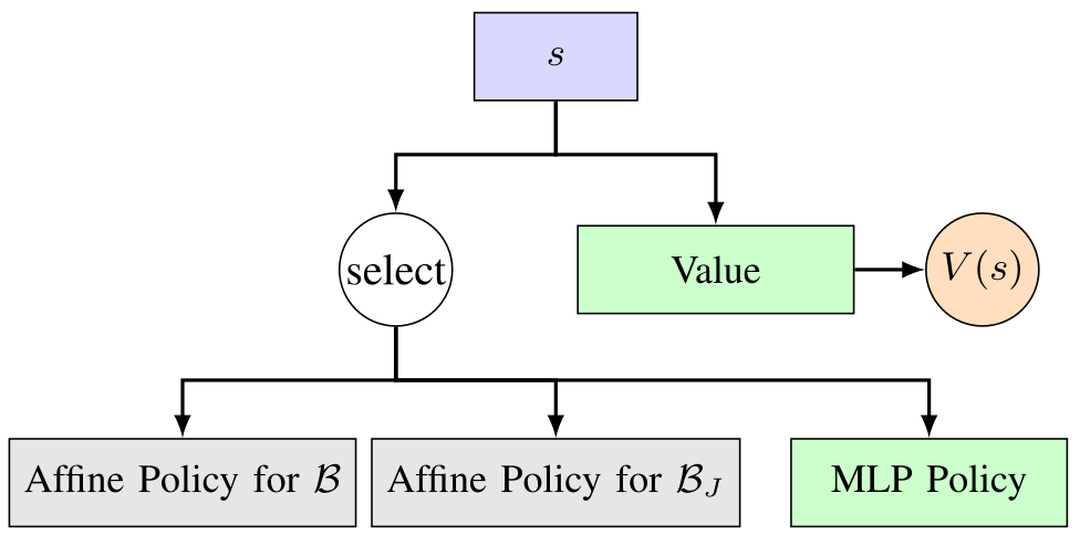
Three actors share a critic: one activation-free linear layer with bias for each buffer, and an MLP elsewhere. A state-dependent selector chooses the actor. The base task actor is trained first without safety considerations, then frozen. Affine actors train from repeated buffer resets using violation penalties while the task actor preserves previously learned behavior.
The paper explicitly separates this training heuristic from verification: safety requires checking the repulsion or dissipation conditions at every buffer vertex using a valid error bound. Training is not guaranteed safe, and an iteration cap is not a certificate of convergence. The source gives no complete treatment of action saturation, competing buffers, boundary switching continuity, or feasibility when actuator limits prevent sufficient repulsion.
V Numerical Simulations
Evaluation uses two low-dimensional deterministic simulators and compares the switched policy with base TD3, CPO and PPO-Barrier. Neither physical hardware nor stochastic disturbances, uncertain resets, high-dimensional modes or nonlinear reset maps are tested. Results concern the stated rollout protocol, not all possible safe initial conditions.
V-A Constrained Pendulum
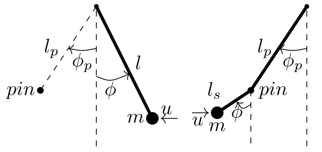
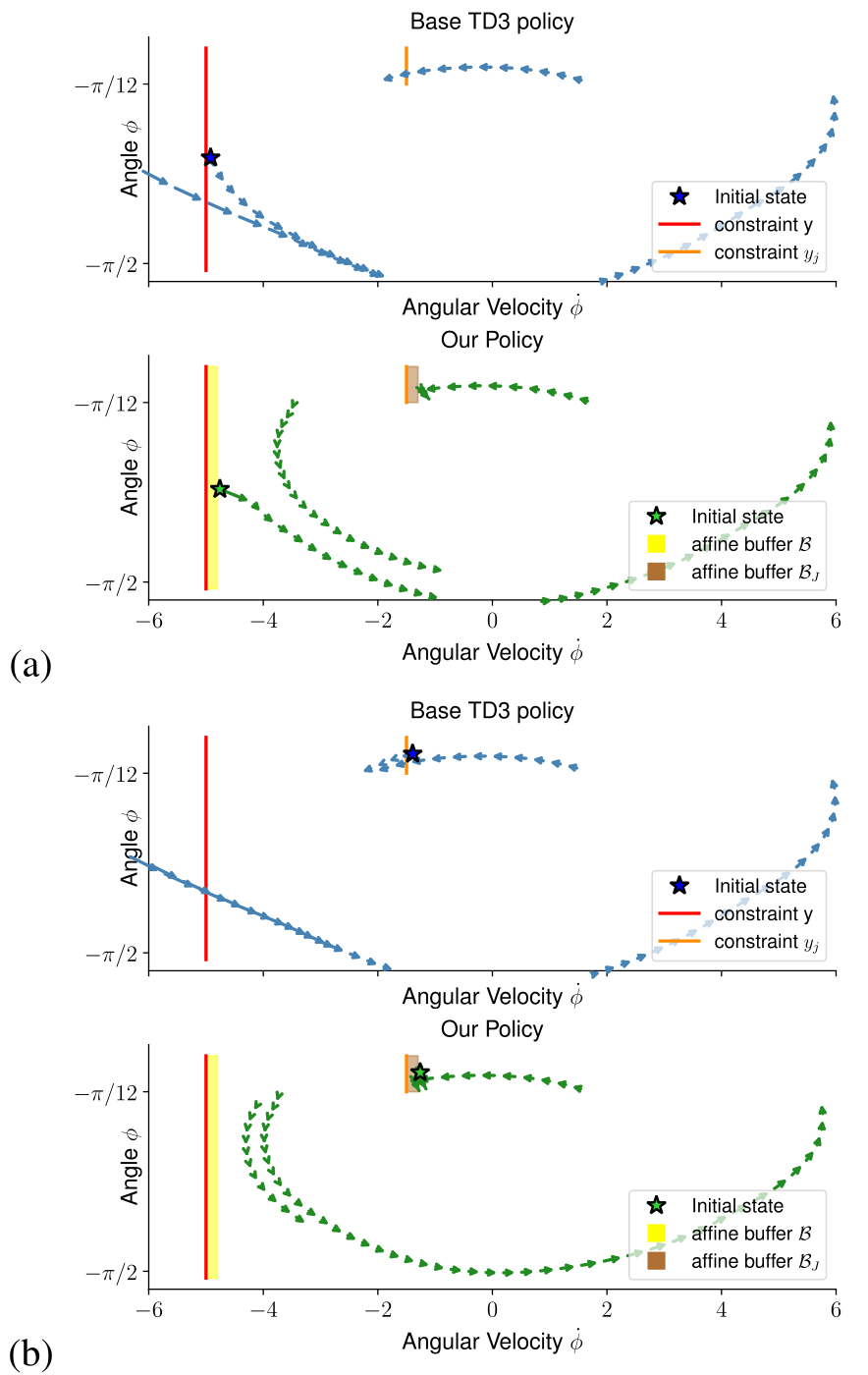
The pendulum changes effective length when it encounters a pin at −π/12, multiplying angular velocity at impact. The task is to reach −π/2 while respecting a velocity boundary in the shortened mode and its transformed pre-impact boundary. Two affine actors handle these regions; the task actor is a three-layer MLP. Main text uses length ratio 3.33, velocity boundaries −5 and −1.5 rad/s, buffer width 0.2 rad/s, and a sample-fitted approximation measure 0.1 rad/s².
Base TD3 trains for about 1,000 iterations, followed by up to 500 affine-actor iterations or completion of the first-order check. The phase portraits show the proposed actors bending trajectories away from the displayed boundaries while reaching the target, unlike the shown TD3 traces.
The source is inconsistent about which side is safe: it first writes velocity≤−5 and the corresponding pre-impact upper bound, but the Figure 5 discussion instead writes velocity>−5 and >−1.5, consistent with the plotted repulsion from large negative speeds. The appendix also changes the length ratio to 3. These are unresolved source conventions, not silently corrected parameters; the reported table is retained as the authors’ evaluation.
V-B Paddle Juggler
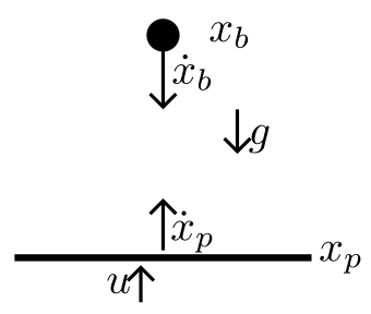
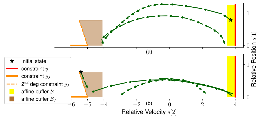
The paddle accelerates under control while the ball falls under gravity. A very heavy paddle is unaffected by impact, and restitution reverses/scales relative velocity. State coordinates are relative distance, relative velocity, paddle position and paddle velocity. The goal is a high ball apex while keeping post-impact relative velocity at most 4 m/s. With restitution 0.8, pre-impact relative velocity below −5 m/s would violate that bound after reset.
Continuous dynamics are affine, so their stated affine-fit residual can be zero. The upper-velocity buffer is 0.5 m/s wide; a second region is intended to dissipate dangerous approach motion before impact. Its actor trains from buffer resets for 1,000 iterations. Figure 7 illustrates both interventions; this qualitative plot is supplemented by the rollout table.
The written transformed output is −e times relative velocity, whose first derivative already contains control under Equation 25. It therefore has relative degree one for e=0.8, despite the paper calling it degree two. Relative distance has degree two, but the connection between a distance-based triangular braking region and the stated transformed output is not fully specified. The main triangular description also differs from the rectangular bounds printed in Equation 28.
V-C Comparison with Baselines
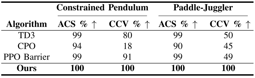
ACS is the percentage of episodes with no constraint violation, whether or not the task finishes. CCV requires both task completion and no violation. The evaluation uses 100 rollouts, split evenly between initializations near the boundary/reset and those farther away.
For the pendulum, ACS/CCV are 99/80 for TD3, 94/18 for CPO, 99/91 for PPO-Barrier and 100/100 for the proposed policy. For the paddle they are 99/50, 90/45, 99/49 and 100/100 respectively. Thus the proposed method has no observed unsafe or incomplete trials in this sample, with CCV gains of nine percentage points over the best listed pendulum baseline and 50 points over the best paddle baseline.
These counts do not prove safety over all trajectories. The source does not report repeated-training seed uncertainty, confidence intervals, detailed task-completion thresholds, rollout duration, apex-height values, returns, learning curves, runtime or full baseline tuning. Most TD3 and PPO-Barrier trials already satisfy the constraint; their larger deficit is completing the task safely.
VI CONCLUSION AND FUTURE WORK
The practical idea is to combine expressive task learning with simple actors in regions amenable to verification, including pre-impact regions. The finite tests show promising safe completion on two simulators. The formal claim remains conditional on exact transition knowledge, valid uniform error bounds, suitable buffer geometry, feasible checked actors and a sound higher-order argument.
The authors identify joint choice of width and approximation error as a limitation: a wider buffer gives more braking room but may require a worse affine approximation and a stronger margin. Automatic buffer selection and humanoid-scale systems are future work. The documented notation and proof gaps should be resolved before treating the general higher-order construction as an implementation-ready certificate.
VII Appendix
VII-A Buffer ℬ is a convex polytope
The appendix writes the buffer as the inverse image of a scalar interval intersected with the mode domain. The interval preimage is an affine strip, and its intersection with a bounded convex polytope is again a polytope. This proof assumes that the mode domain is such a polytope; that does not follow merely from the earlier statement that it is a subset of the state space. The proof’s width symbol r corresponds to the main text’s w.
VII-B Proof of Theorem 2
The proof first transfers a vertex margin to an affine acceleration approximation, then uses convex combinations to reach the buffer interior. Its last interpolation step replaces the weighted sum of derivatives at vertices by the derivative at the interpolated state. For general nonlinear dynamics, that equality is not implied by an affine policy. Moreover, β times a state-derivative vector cannot be subtracted from a scalar output acceleration without an explicit projection or suitable output coordinates.
Even if the intended interior inequality ÿ≤−βẏ is separately established, it bounds velocity exponentially; it does not yield Equation 18’s claimed bounds for both derivative orders or its extra strict inequality. A sufficient braking argument additionally needs the entry condition ẏ≤β(d−y). With that condition, h=ẏ+β(y−d) has ḣ≤0 and the envelope remains valid while the condition holds. This explains the intended mechanism without claiming that the printed proof establishes every required assumption.
Equations 15–18
| (15) | ||||
| (16) |
| (17) |
| (18) |
VII-C Buffer Design for Relative Degree 2 Buffer
The proposed envelope allows approach speed proportional to remaining distance: ẏ≤β(d−y), with β set by maximum speed at the outer buffer edge. At the constraint boundary this reduces to nonpositive approach speed. A compact polytope bounds the other coordinates. The unnumbered lower/upper-bound display and Equations 19–22 are preserved.
Equation 21 is a sufficient condition for preserving that envelope from a valid entry, not a consequence obtainable by freely differentiating an arbitrary inequality. A triangular polytope in output/velocity coordinates need not remain a polytope under an unspecified nonlinear mapping to the original state. The source also introduces inconsistent or undefined coordinate symbols and does not fully analyze entry from other faces or finite-time exit; non-crossing need not imply eventual exit.
Equations 19–22
| (19) |
| (20) |
| (21) |
| (22) |
VII-D Numerical Simulations Details
VII-D 1 Constrained Pendulum
The simulator uses gravity, viscous damping and control acceleration for the pendulum, with a reset that fixes the impact angle and scales angular velocity. The reverse reset divides velocity by the length ratio. This appendix sets the short length to one third of the original and hence ratio three, whereas the main text uses 3.33. A −5 rad/s boundary would transform to −5/3 under the appendix ratio rather than the main −1.5.
Rectangular buffers bound angle and velocity around the post-impact and pre-impact boundaries. Both stated velocity constraints are first order. Several notation problems remain: a scalar inequality is assigned a vector d, unsafe jump sets use ≤ where Definition 2 uses >, and the velocity signs disagree with the phase-portrait discussion. Exact displays are retained so readers can distinguish these source discrepancies from the reported empirical results. Numerical masses, damping, action bounds, integration timestep and detailed reward are not fully supplied.
Equations 23–24
| (23) |
| (24) |
VII-D 2 Paddle Juggler
The original-coordinate reset changes ball velocity to (1+e) times paddle velocity minus e times ball velocity. In relative coordinates only the relative velocity is multiplied by −e. Equation 25 gives relative acceleration −g−u and paddle acceleration u; distance derivatives follow the corresponding velocities. Ball and paddle start with zero velocity, and the paddle starts at zero position.
The continuous buffer bounds relative distance in [0,5], relative velocity in [3.5,4], paddle position in [−1,1] and paddle velocity in [−5,5]. Equation 28 gives jump-buffer bounds [0,0.77], [−5.5,−5], [−1,1] and [−5,5]. These are printed as a rectangular product, not the triangular envelope described earlier. The prose also writes a generic endpoint −e times the velocity limit, which differs from the correct pre-impact threshold −limit/e and from the numeric −5.
The appendix repeats vector/scalar threshold and unsafe-set-sign inconsistencies. Its explicitly defined transformed output has relative degree one; a different distance-based second-order output would need an explicit definition and verified connection to impact safety. The complete source dynamics and bounds are preserved, but the paper alone does not resolve which inconsistent convention was used by the implementation.
Equations 25–28
| (25) |
| (26) |
| (27) | ||||
| (28) | ||||