At a glance
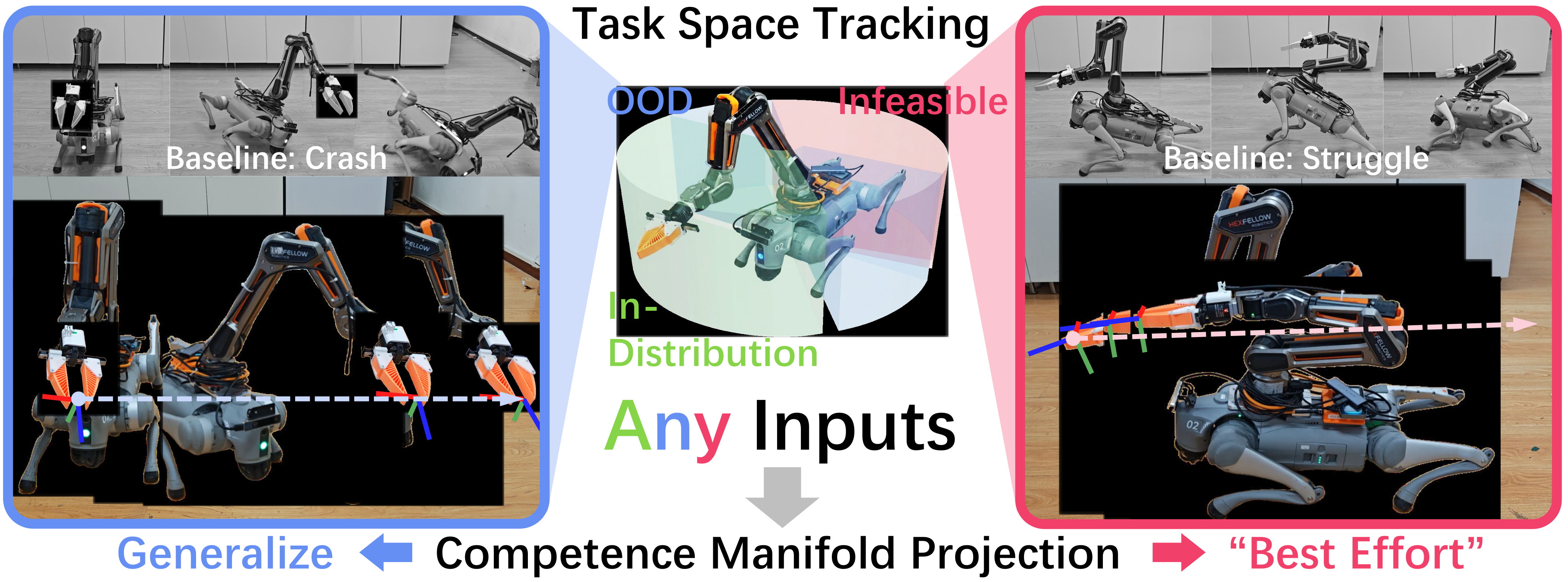
CMP adds a learned latent-command filter to whole-body end-effector tracking. Training encourages safer intentions to occupy smaller latent radii, so deployment can limit commands with a single radial projection rather than iterative safety optimization. At the selected radius, simulation survival rises from 4.7% to 46.9% for rear-workspace commands and from 6.9% to 40.3% for corrupted sensor inputs. The physical robot survives 42 of 45 trials, with tracking accuracy traded against survival. These are empirical robustness results, not certified safety for arbitrary commands.
I Introduction
Global end-effector commands let one controller coordinate legs and arm through interfaces such as UMI-on-Legs and UMI. However, noisy localization or unfamiliar targets can demand motions that the policy never mastered. Training-set membership alone does not identify this competence boundary: familiar examples can still fail.
CMP learns a safety value alongside a state-conditioned intent encoder and tracking policy, then shapes latent geometry so a radius threshold approximately selects safer intentions. The objective is continued motion with reduced ambition rather than abrupt rejection. This edition covers all 14 pages of v1, dated 8 April 2026, including all eight figures, six numbered tables, 17 numbered equations, the full appendix proof and 58 references.
II Related Work
II-A Whole-Body Control for Legged Manipulators
Modular locomotion/manipulation controllers simplify control and transfer, while unified policies can exploit whole-body coordination. Global-pose tracking improves compatibility with manipulation datasets but exposes the controller to bad relative targets from state estimation or users. CMP keeps a unified policy and modifies its latent input; the experiments do not establish that every modular design necessarily has inferior workspace or task performance.
II-B Physical Safety and OOD Handling
Recovery policies react to failure, while predictive safety filters, barrier functions and reachability methods try to intervene earlier. Learned failure detectors often stop rather than repair commands. CMP compares with latent-space shielding and a learned latent control barrier function, replacing their runtime checks or optimization with an encoder trained to organize safer intentions radially. Its speed advantage is measured for these implementations, not a universal impossibility result for other safety methods.
III Problem Formulation
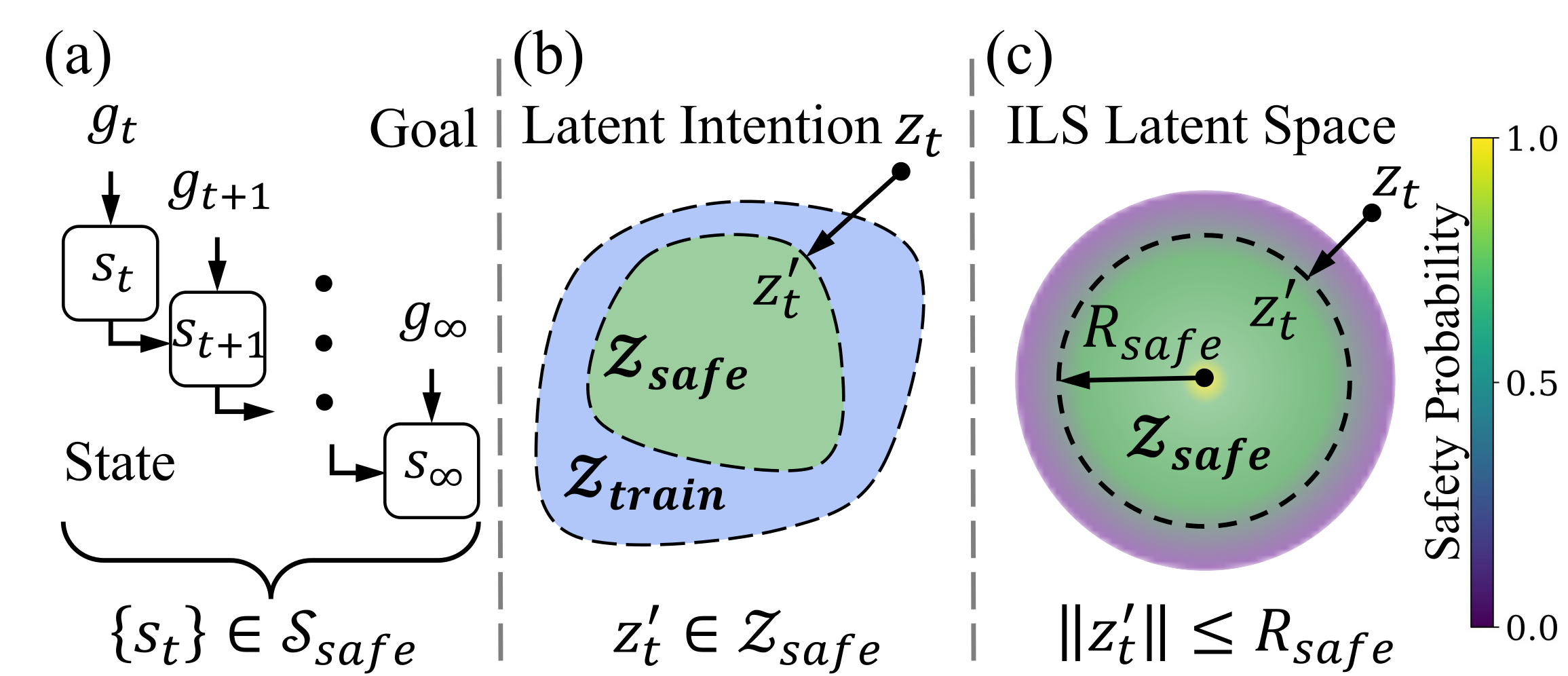
The desired controller remains in a designated safe state set despite arbitrary goal sequences. A learned competence set depends jointly on state and goal, rather than only on the training distribution. CMP seeks a minimally disruptive modification of unsafe intentions. The paper’s formal set is broader than the experimental termination rule: the latter primarily detects forbidden body contacts, while joint limits, torque saturation and action rates are soft penalties.
Safety cannot be recovered from every conceivable initial state; a state already outside the safe set violates the objective immediately. The practical question is which commands preserve recoverability from the current state, under the learned policy and modeled dynamics.
Equation 1
| (1) |
IV Method
IV-A Overview
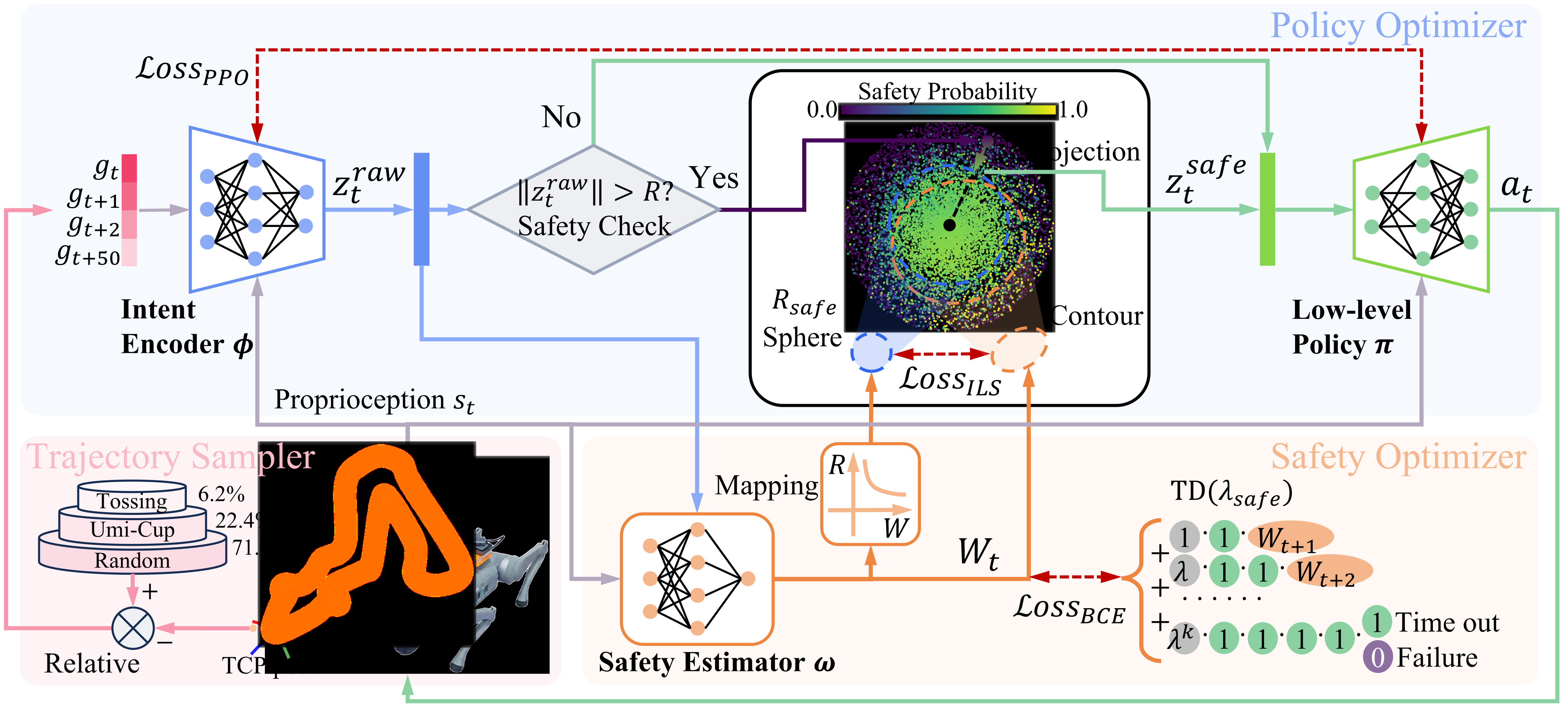
A state-conditioned encoder maps trajectory goals to latent intentions, and a low-level policy turns state plus intention into 18 leg/arm actions. A separately optimized estimator scores state–intention pairs. The encoder and policy share task training, while geometric regularization uses safety targets. The formulation treats a single observation as the state and omits history, so its Markov analysis assumes that this representation contains the information needed for prediction.
IV-B Frame-Wise Safety Scheme
Inspired by conditional latent models, the encoder outputs a Gaussian intention and the policy conditions on the sampled code and current state. PPO jointly trains the two networks. The theoretical value W(s,z) commits to the current intention and then maximizes survival probability over future intentions; its Bellman equation multiplies the current safe-state indicator by the next optimal value.
The competence set consists of intentions whose optimal-continuation value is at least 1−δ. Membership exactly expresses the existence of a sufficiently safe continuation. It does not by itself guarantee that repeatedly choosing arbitrary members achieves that probability forever: for δ>0, repeatedly taking a risky action can accumulate failure risk even when a safe continuation was available after each step. This distinction concerns the formal claim, not a demonstrated cause of the reported hardware failures.
Equations 2–4
| (2) |
| (3) |
| (4) |
IV-C Lower-Bounded Safety Estimator
The estimator replaces an expensive maximization over future intentions with its prediction at the latent origin. Backward TD(λ) targets mix this bootstrap value with later returns, using λ=0.8; failures receive zero and timeouts receive one. Binary cross-entropy fits the predicted probability independently of the tracking-policy optimizer.
The appendix derives conservative expected targets when the continuation values are exact. A fitted neural value is not automatically a lower bound and can overestimate, as the paper’s failure analysis acknowledges. Assigning one at a finite timeout also supervises survival to the episode horizon; it does not observe or certify perpetual safety beyond that timeout.
Equations 5–7
| (5) |
| (6) |
| (7) |
IV-D Isomorphic Latent Space
ILS makes safety filtering inexpensive by encouraging latent norm to correlate inversely with predicted safety. It is a statistical organization learned through regularization. It does not establish a bijective, distance-preserving map between original goals and a certified safe ball, despite the term “isomorphic.”
IV-D 1 Mapping Construction
A clipped inverse-cubic function maps the safety target to a Gaussian prior scale. The denominator includes ε=1−the batch-average safety, centering its typical value around one. Lower predicted safety produces a larger scale, while minimum and maximum clipping limit extreme gradients. The numerical clipping bounds and a calibrated correspondence between radius and failure probability are not provided.
Equation 8
| (8) |
IV-D 2 Implicit Isomorphism
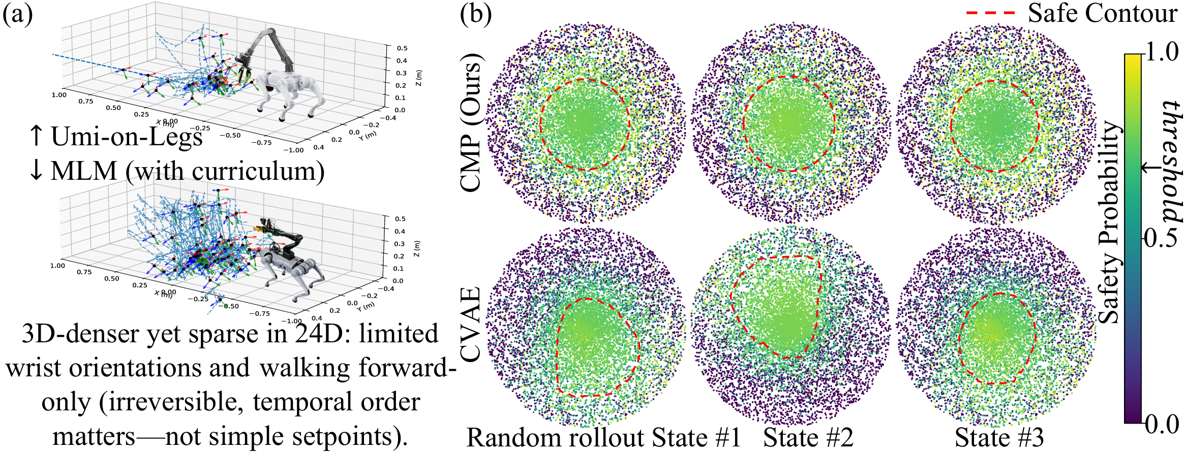
KL regularization matches each encoded Gaussian to an isotropic prior with safety-dependent variance. For an exact d-dimensional isotropic Gaussian, typical norm scales as √d times the standard deviation; this motivates radial organization. Finite-dimensional distributions overlap, and approximate KL matching does not make every point at a given radius equally safe. The three-state visualization supports a learned correlation rather than a universal geometric certificate.
Equation 9
| (9) |
IV-D 3 Runtime Competence Manifold Projection
Runtime projection scales an over-radius code down to the selected boundary and otherwise leaves it unchanged. This exactly projects onto a Euclidean latent ball and needs no iterative optimizer or estimator call. For fixed network and latent sizes the work per command is fixed; computing a norm and rescaling is linear in latent dimension if that dimension varies.
Clipping guarantees the norm bound, not that the learned ball equals the true safe set or that Euclidean proximity is the nearest goal under a task-semantic metric. Smoothly changing latent codes can produce useful partial tracking, but the paper reports failures from imperfect mapping. Radius is a runtime trade-off parameter rather than a calibrated probability guarantee.
Equation 10
| (10) |
V Simulation Experiments
Isaac Gym simulates a Unitree Go2 quadruped with a Hexfellow Saber arm and UMI gripper. Evaluation covers familiar trajectories, rear-workspace commands and injected localization errors. This changes commanded inputs while retaining the modeled robot/environment; it is not a test of arbitrary dynamics shifts.
V-A Overall Performance Comparison
Each scenario contains 7,000 trajectories and results are reported over three seeds. Main text rounds duration to 13 seconds; the appendix specifies 2,500 steps at 200 Hz, or 12.5 seconds. Survival means no early termination. Tracking errors are omitted when survival is below 30%, limiting comparisons in the hardest settings; omission does not by itself eliminate survivorship effects among reported runs.
At radius 2, CMP gives ID survival 94.7%, position error 4.5 cm and orientation error 0.106 rad. UMI-on-Legs gives 85.3%, 4.9 cm and 0.105 rad; Neural CBF has higher ID survival, 95.9%. Rear-workspace survival is 46.9% versus 4.7%, about 9.98× rather than exactly 10× from the displayed values. Sensor-corruption survival is 40.3% versus 6.9%, about 5.84×. CMP’s remaining rear-workspace errors are large: 79 cm and 1.661 rad.
Radius matters substantially. Radius 1 raises rear survival to 82.5% but yields 102.2 cm rear error and 15.6 cm ID error. Near-unclipped radius 100 has 3.5 cm ID error but only 5.1% rear survival. Compared with that same-policy setting, selected-radius ID position error increases about 28.6%; the headline “under 10%” is not a uniform bound across radii, metrics or comparison choices. Explanations of baseline failure mechanisms are author interpretations without a separate causal ablation.
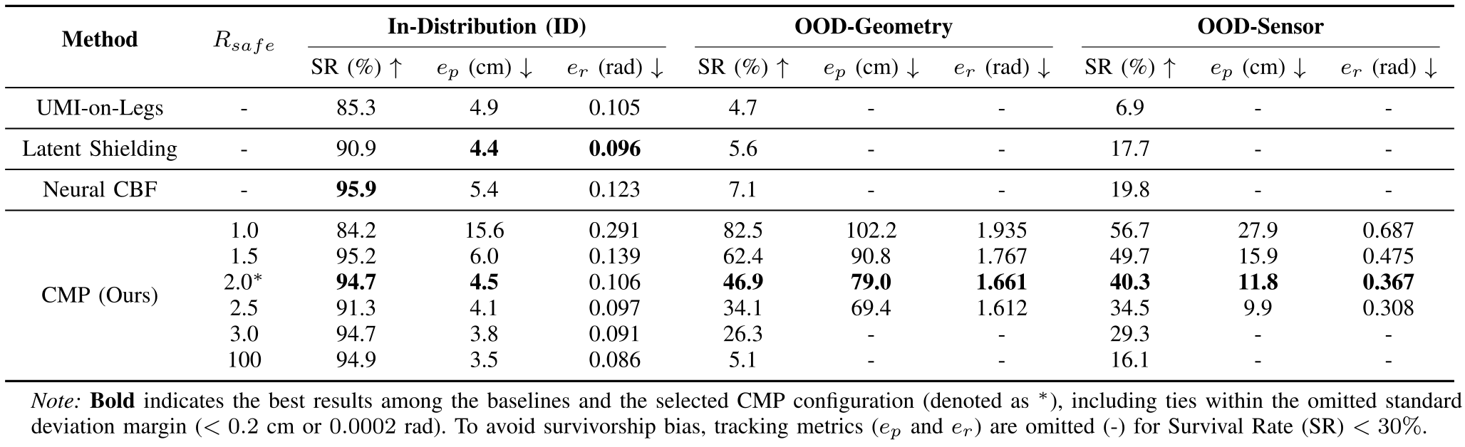
Original selectable table and notes
| Method | In-Distribution (ID) | OOD-Geometry | OOD-Sensor | |||||||
| SR (%) | (cm) | (rad) | SR (%) | (cm) | (rad) | SR (%) | (cm) | (rad) | ||
| UMI-on-Legs | - | 85.3 | 4.9 | 0.105 | 4.7 | - | - | 6.9 | - | - |
| Latent Shielding | - | 90.9 | 4.4 | 0.096 | 5.6 | - | - | 17.7 | - | - |
| Neural CBF | - | 95.9 | 5.4 | 0.123 | 7.1 | - | - | 19.8 | - | - |
| CMP (Ours) | 1.0 | 84.2 | 15.6 | 0.291 | 82.5 | 102.2 | 1.935 | 56.7 | 27.9 | 0.687 |
| 1.5 | 95.2 | 6.0 | 0.139 | 62.4 | 90.8 | 1.767 | 49.7 | 15.9 | 0.475 | |
| 2.0∗ | 94.7 | 4.5 | 0.106 | 46.9 | 79.0 | 1.661 | 40.3 | 11.8 | 0.367 | |
| 2.5 | 91.3 | 4.1 | 0.097 | 34.1 | 69.4 | 1.612 | 34.5 | 9.9 | 0.308 | |
| 3.0 | 94.7 | 3.8 | 0.091 | 26.3 | - | - | 29.3 | - | - | |
| 100 | 94.9 | 3.5 | 0.086 | 5.1 | - | - | 16.1 | - | - | |
V-B Ablation Studies
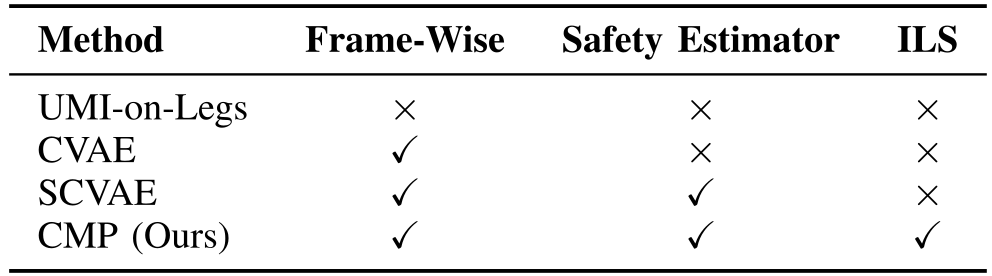
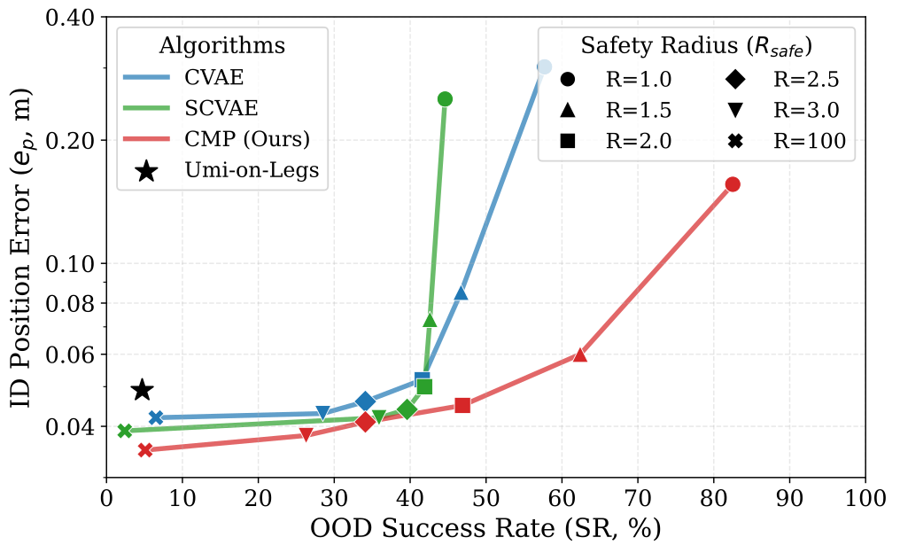
CVAE truncates a conventional latent distribution. SCVAE applies KL only to samples whose estimated safety exceeds the batch mean. CMP additionally shapes prior variance by safety. The radius sweep compares OOD-geometry survival against ID position error, supporting a better observed trade-off for the structured latent space.
SCVAE can worsen sharply under strong truncation because its center is not explicitly organized for safety. Smaller radius is not universally better: even CMP’s ID survival at radius 1 is below its selected-radius result. Figure 4 labels its horizontal axis “Success Rate,” while its caption and experimental metric define SR as survival; it should not be read as task completion.

Original selectable table and notes
V-C Validation of Safety Estimator
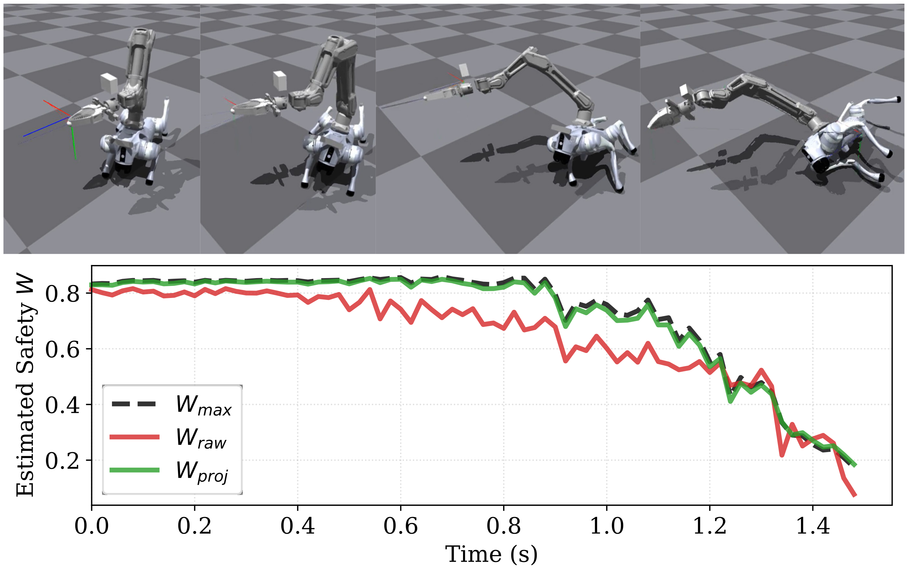
A qualitative rollout executes raw, unprojected commands. Origin, projected-code and raw-code scores are initially high; after an unfamiliar sideways target the raw score is lower, and near a fall all three decline. The projected score is evaluated counterfactually along the raw execution, not evidence that the projected rollout was executed in this figure. It illustrates sensitivity to state and intent; quantitative validation uses human judgments in Appendix D.
VI Real-world Experiments
VI-A Experimental Setup
The physical Go2 carries a six-DoF Saber arm. The UMI gripper is removed for all safety-critical evaluation, so the tasks test motion tracking rather than demonstrated object manipulation with that gripper. A RealSense T265 supplies global base localization; preset global target poses become relative policy inputs. Drift and infeasible user targets can therefore both create unfamiliar relative commands.
VI-B Robustness to OOD Commands
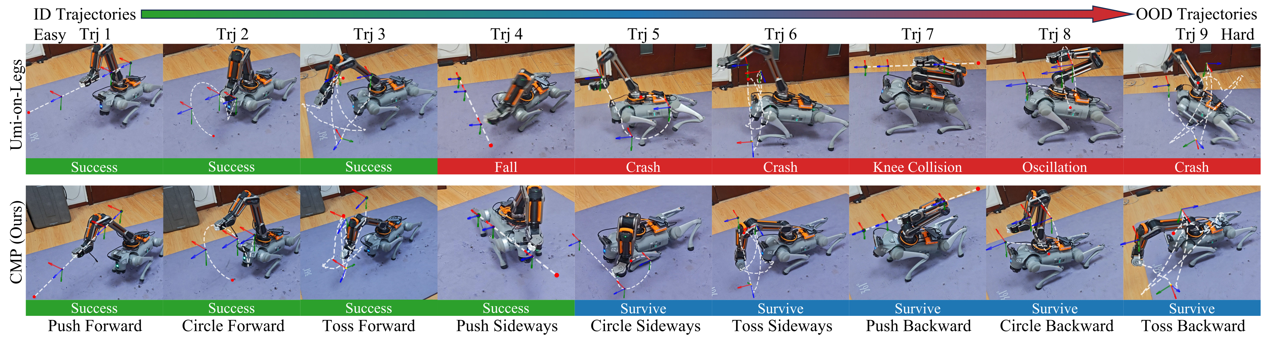
There are 15 target trajectories, five in each difficulty class, with three trials each: 45 trials per method. CMP survives 15/15 ID, 14/15 moderate OOD and 13/15 extreme OOD trials, or 42/45 overall. UMI-on-Legs survives 12/15 ID and none of either OOD category; latent shielding achieves 11/15, 5/15 and 3/15; Neural CBF achieves 12/15, 9/15 and 6/15. Survival and task success remain distinct, as the green/blue labels in Figure 6 show.
CMP’s ID position error is 5.1±1.8 cm versus UMI’s 4.9±1.6 cm, about a 4.1% increase; orientation error is 0.09±0.03 versus 0.07±0.02 rad, about a 28.6% increase in the means. Thus “under 10% tracking degradation” does not apply to every listed metric. Overlapping spreads are not a formal significance or equivalence test. Moderate/extreme CMP errors are 9.6/19.2 cm and 0.24/0.87 rad, showing survival at reduced fidelity.
Reported latency is 2.99±0.14 ms for CMP versus 2.97±0.15 ms unfiltered, 3.89±0.49 ms shielding and 5.36±0.54 ms Neural CBF. These implementation measurements show small CMP overhead; they do not alone prove all alternatives miss a particular control deadline. Of CMP’s three failures, the authors attribute one to estimator overprediction and two to imperfect spherical mapping. Payload or dynamics disturbances are outside the demonstrated scope.
VI-C Robustness to Sensor Divergence
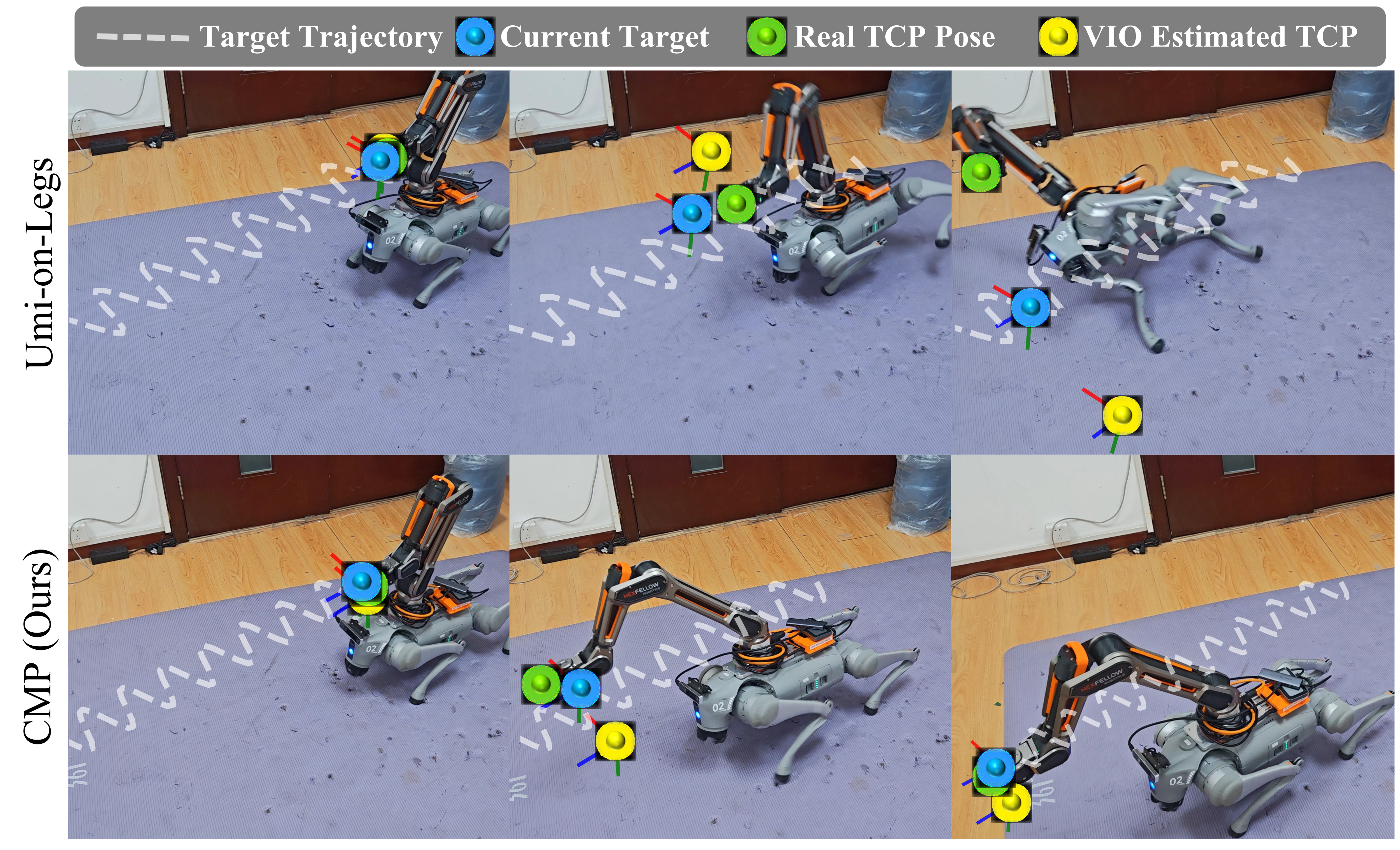
A sinusoidal tracking example provokes fast lateral adjustments and localization drift. The baseline responds aggressively to distorted targets, producing a feedback loop of motion and larger estimation error; CMP attenuates unfamiliar intentions and remains stable in the shown sequence. This is a qualitative illustration, without a quantitative sensor-bandwidth or drift-error sweep establishing the cause for every failure.
VII Conclusion
CMP offers a practical, inexpensive command filter that substantially improves survival in the reported shifts while retaining partial motion intent. Its central limitation is the gap between ideal optimal-continuation values and learned finite-horizon targets plus an approximate radial map. The authors propose humanoid scaling and online radius tuning; neither is evaluated here. The result supports empirical robustness on this robot and benchmark, not unconditional safety under arbitrary inputs or dynamics.
Appendix
VII-A Necessity of Latent Space Safety
Four six-DoF keyframes already form a 24-dimensional command space, where apparently dense 3D trajectories cover only a small part of the possible sequences. Order, kinematic singularities and base reorientation complicate direct constraints. This motivates a compact learned intent space, but dimensionality alone is not a formal proof that every direct feasibility algorithm is computationally intractable.
VII-B Visualization of Isomorphic Latent Space
PCA views compare learned latent organization for three sampled states. CMP’s scores appear more radially ordered than the conventional representation, consistent with the intended regularization. A 2D projection and three states cannot establish safety of every latent direction or a globally spherical boundary; the experiment is illustrative rather than a calibration certificate.
VII-C Proof of Lower Bound Property
The complete proof is preserved. It analyzes expected rollout survival with exact optimal continuation values, then forms a weighted mixture of those quantities. This is a useful idealized lower-bound argument; replacing exact values by learned estimates and finite timeouts requires additional assumptions not proved here.
VII-C 1 Definitions
V*(s) maximizes the safety value over the next latent intention. The multiplicative Bellman equation combines the current safety indicator with expected V* at the next state. These quantities assume the fixed low-level policy, correct dynamics and future controls chosen to optimize survival.
Equations 11–12
| (11) |
| (12) |
VII-C 2 The n -step Expansion Operator
The n-step quantity follows the rollout intentions for n steps and then uses optimal continuation. Products of state-safety indicators make a failed trajectory contribute zero. With the first intention fixed and exact continuation values, the one-step expression equals the ideal W value.
Equation 13
| (13) |
VII-C 3 Monotonicity Proof
Replacing one optimal future choice with the rollout policy cannot improve its expected safety value. Applying this inequality inside the nonnegative indicator product yields P(n)≥P(n+1). The result compares expected values under the stated model; it is not a pointwise guarantee for every sampled trajectory or fitted prediction.
Equations 14–15
| (14) |
| (15) |
VII-C 4 TD( λ s a f e ) Target and Tightness
For 0≤λ<1, geometric weights form a convex mixture of the n-step expectations, hence the mixture is no greater than the first term. The displayed inequality is non-strict and equality is possible, despite the text calling it a “strict lower bound.”
Larger λ propagates failure signals farther and relies less on early bootstraps, but increases variance and moves toward the rollout policy’s more conservative survival value. Smaller λ propagates failures slowly and depends more on estimator quality. The chosen λ=0.8 is a practical balance rather than a proven optimum.
Equations 16–17
| (16) |
| (17) |
VII-C 5 Approximation of the Maximization (Eq. ( 5 ))
The exact origin value cannot exceed the exact maximum over all intentions, so substituting that exact value is conservative. Substituting a learned estimate is only conservative if its estimation error also respects the bound. The proposed feedback between KL organization and estimator training may improve origin quality, but qualitative peak alignment does not prove a uniform approximation error bound.
VII-D Quantitative Validation of Safety Estimator
Five human evaluators label 500 sampled OOD rollout states as salvageable or unsalvageable. The low-score bin contains 84 states judged unsalvageable and two salvageable, giving 97.7% agreement with an unsalvageable interpretation. The high-score bin contains 289 salvageable and seven unsalvageable states, giving 97.6% agreement with a salvageable interpretation.
The middle bin contains 118 states, 46 labeled salvageable and 72 unsalvageable. These statistics measure correspondence with human judgments, not recovery outcomes under optimal controls or calibrated infinite-horizon probabilities. Vote aggregation and inter-rater agreement are not detailed. The full six-cell table is retained.

Original selectable table and notes
| Human Label | |||
|---|---|---|---|
| Salvageable | 0.4% | 9.2% | 57.8% |
| Unsalvageable | 16.8% | 14.4% | 1.4% |
VII-E Dataset Generation Details
All trajectories are standardized to 2,500 samples at 200 Hz, lasting 12.5 seconds; the main experiment text rounds this to 13 seconds. The initial robot faces +x and gravity points along −z. The training set combines augmented recorded motions with procedural trajectories.
VII-E 1 In-Distribution (ID) Dataset
The training dataset consists of 7,000 trajectories, constructed from two primary sources:
Augmented UMI Data
The source pool has 1,090 “cup in the wild” and 101 tossing trajectories from UMI-on-Legs. Tossing is oversampled threefold, and 2,000 augmented trajectories are drawn from the resulting pool; this is not 2,000 unique recordings. Centered trajectories receive x translations in [−0.2,0.2] m and yaw rotations in [−30°,30°] about a pivot at (−0.3,0,0) m.
Procedural Random Pushes
The remaining 5,000 training trajectories are random pushes. Horizontal steps are 0.1–0.5 m within ±45° of forward, with speed 0.01–0.4 m/s. Height ranges from 0.02 to 0.6 m with vertical speeds 0.01–0.2 m/s. Orientations interpolate roll ±30°, pitch 15–60° and yaw ±45° at 0.01–1 rad/s. A separate ID test set uses the same protocol with different seeds.
VII-E 2 Out-of-Distribution (OOD) Datasets
We evaluate generalization using two challenging variants, each containing 7,000 trajectories derived from the full ID dataset.
OOD-Geometry (Rear Workspace)
The rear-workspace set resamples the full ID collection 7,000 times and changes augmentation yaw to 179–181°. This rotates the frontal motion distribution toward the rear and can require whole-body reorientation. The broad 120–240° range in the main description characterizes resulting targets, while the appendix’s 179–181° is the added rotation; they are different quantities.
OOD-Sensor (Drift & Jumps)
The sensor set adds persistent command bias at random intervals of one to five seconds. Position perturbations have Gaussian standard deviation 0.2 m; Euler-angle perturbations have standard deviation 30° and are composed as rotations. Each event affects the remaining trajectory, so this models accumulated jumps/drift rather than independent framewise measurement noise.
VII-F Termination Conditions
Episodes terminate when a risk-sensitive non-foot body contacts the environment with force above 1 N. Listed links include base, hips, thighs, head and all arm segments; feet may contact the ground. Joint limits, torque saturation and action rates instead incur reward penalties. Survival therefore indicates only absence of the specified early-termination event during evaluation, not satisfaction of every operational constraint.
VII-G Implementation Details
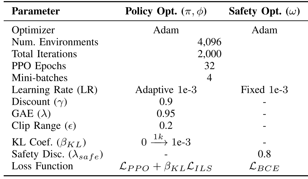
Training uses PyTorch on one NVIDIA RTX A6000 for approximately 2.5 hours and 2,000 iterations. The paper supplies architecture and optimization tables, but details such as exact radius-to-confidence calibration and statistical guarantees for the learned estimator remain absent.
VII-G 1 Network Architectures
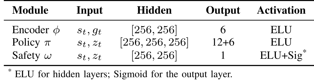
The intent encoder and safety estimator each use two 256-unit hidden layers; the policy uses three. Table V reports encoder output size six, policy output 12+6 and estimator output one. Hidden activations are ELU, with a sigmoid safety output. The main Gaussian-encoder description does not fully specify how means/covariances or sampling versus deterministic deployment correspond to that listed encoder output.
VII-G 2 Training Hyperparameters
Separate Adam optimizers train policy/encoder and safety value across 4,096 environments. The table lists 32 PPO epochs and four minibatches, adaptive policy learning rate 10⁻³ and fixed safety rate 10⁻³. Policy discount is 0.9, GAE λ is 0.95 and clipping is 0.2. The KL coefficient ramps from zero to 10⁻³ over 1,000 iterations; safety TD λ is 0.8. Policy loss combines PPO and weighted ILS, while the estimator uses binary cross-entropy.