Overview
This edition covers all twenty-one pages of arXiv v2, dated 8 September 2026, including Appendices A–G. The thirteen authors are affiliated with Sun Yat-sen, Peking, Tsinghua and Stanford universities and Jiangxing Intelligence. All twelve figures, eight data tables, mathematical definitions and references are retained.
At a glance
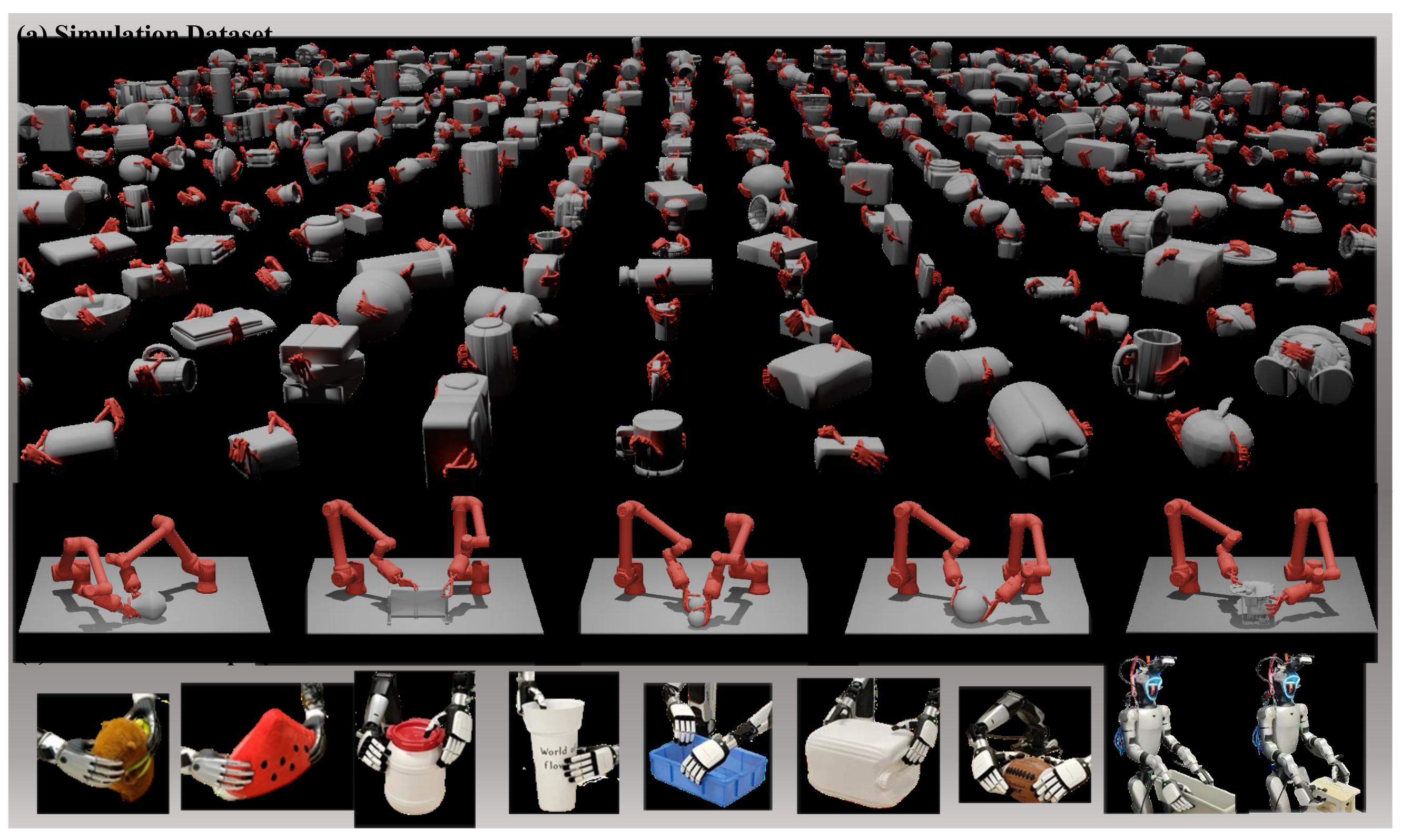
BiDexGrasp combines a synthetic dataset of 9.53 million bimanual grasps over 6,351 objects with a model that generates coordinated two-hand poses for unseen objects. Objects span eleven sizes from 30 to 80 cm.
Synthesis ranks plausible contact-region pairs before optimizing each hand’s grasp quality and checking reachability. The learned model selects compatible approach views, anchors each wrist to object scale and diffuses relative hand poses using local geometry. Reported success is 66.8% in the main simulated generation test and 74.6% across 260 real trials; these use different protocols.
1 Introduction
Two dexterous hands expand both useful object coverage and the search space. Independent single-hand candidates often collide, miss compatible contact regions or assign nearly all support to one hand.
The proposed solution addresses dataset construction and learned generation separately. Its synthetic poses cover geometry, scale, pre-grasp execution and feasible arm configurations; the learned generator predicts floating-hand grasps, with arm motion and hand retargeting handled afterward. Dataset size is a count of synthesized poses, not independent real executions.
2 Related work
The related work distinguishes bimanual control, synthetic grasp datasets and learned pose generators. Comparisons depend on hand embodiment, object scale, tabletop support and whether arm reachability is included.
2.1 Bimanual Dexterous Grasp
Bi-DexHands and ArtiGrasp study bimanual manipulation through learned control, while BimanGrasp and other data-driven methods synthesize or predict grasps. BiDexGrasp targets efficient paired-pose generation over varied objects rather than a general dexterous manipulation policy.
2.2 Dexterous Grasp Dataset
DexGraspNet and BODex show the value of large synthetic single-hand datasets. Extending them to two hands adds joint coordination and collision constraints. Table 1 retains the source’s coverage comparison, including object counts, scale ranges, tabletop support, IK and pre-grasp annotations.
The reported 9.53 million poses cover 6,351 base objects at multiple scales. Table 1’s claim of independence from preexisting single-hand grasp data does not imply independence from existing object-mesh collections.
| Dataset | Bim. | Obj | Grasp | Max | Range | Table | IK | Pre-Grasp | Data Independent |
| DexGraspNet[33] | 5355 | 1.32M | 30cm | 28cm | ✓ | ||||
| BODex[4] | 2397 | 3.08M | 24cm | 12cm | ✓ | ✓ | ✓ | ✓ | |
| DHAGrasp[19] | ✓ | 802 | 1.30M | 30cm | 20cm | ||||
| BimanGrasp[28] | ✓ | 900 | 0.15M | 40cm | 20cm | ✓ | |||
| BiDexGrasp | ✓ | 6351 | 9.53M | 80cm | 50cm | ✓ | ✓ | ✓ | ✓ |
2.3 Data-Driven Dexterous Grasp Framework
Prior generators use diffusion, transformers, contact representations, language or physical losses. Inspired in part by DexGraspNet 2.0, this work explicitly selects coordinated views and predicts relative poses around geometry/scale-adaptive anchors.
3 Preliminaries
A contact force constrained by friction maps through a grasp matrix to a six-dimensional force/torque wrench. Summing feasible contact-wrench sets gives the grasp wrench space (GWS). The origin-to-boundary margin is a useful stability measure when interpreted with origin containment and the assumed contact model.
QP energy measures squared distance from selected target disturbances to feasible grasp wrenches. Lower residual means better resistance to those targets. The text describes six ±x/y/z disturbances but also calls them six orthogonal axes in the supplement; this finite test should not be treated as a certificate of robustness to every six-dimensional disturbance.
Equations
4 BiDexGrasp Dataset
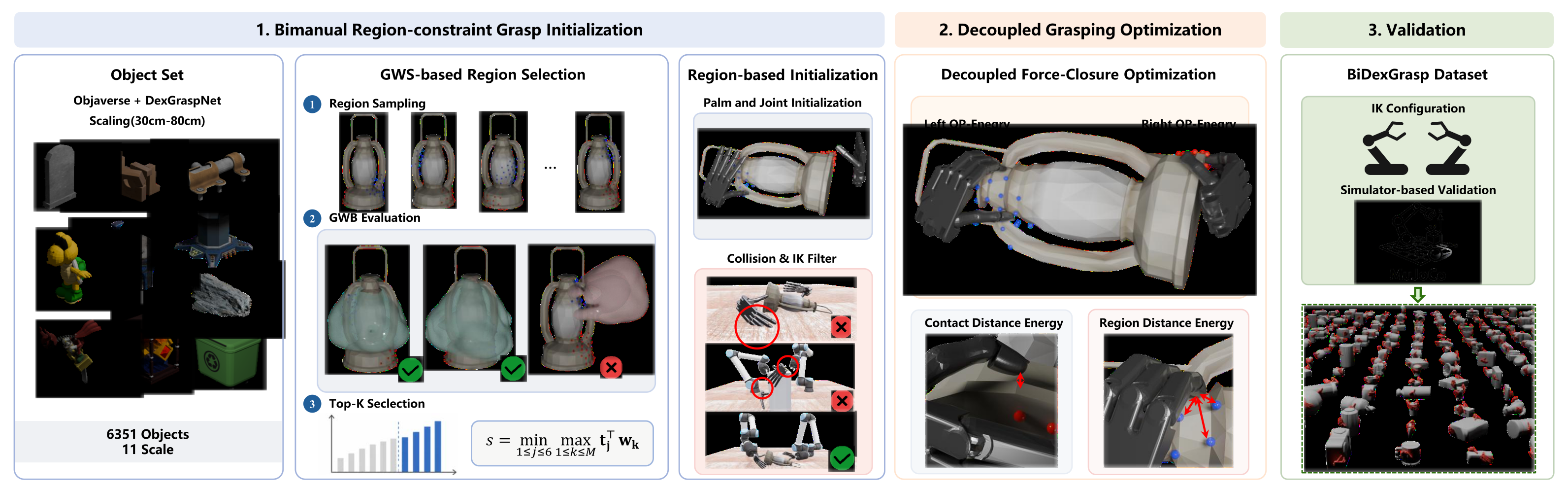
The synthesis pipeline first initializes coordinated regions, then optimizes contact quality and finally constructs feasible arm-hand execution configurations.
4.1 Overview
Represent each hand by wrist translation, wrist rotation and finger joints; the bimanual pose contains both. Collect 6,351 meshes from DexGraspNet and Objaverse and scale each to eleven sizes between 30 and 80 cm. The original left/right tuple ordering is retained exactly in the formal definition.
Equation
4.2 Bimanual Region-constraint Grasp Initialization
Use farthest-point sampling for 200 surface anchors, with 256 points in an 8-cm neighborhood defining each region. Remove region pairs closer than 5 cm. For each remaining pair, sample five contacts per region and estimate 1,000 wrench-boundary samples with the TDG estimator.
Score a pair by its worst support projection over the six tested disturbances and retain the top forty. This sampled directional score ranks candidate regions; it is not the exact minimum margin over all possible wrench directions.
Place each palm near its region on a dilated convex hull, align its normal to the surface and choose a favorable arm orientation. Reject collisions and unreachable wrist configurations before optimization. Figure 2 preserves the complete initialization–optimization–validation pipeline.
Equation
4.3 Decoupled Grasping Optimization
Equation 1 adds separate left/right QP energies, contact-to-object distance and region-consistency penalties. Separating the quality terms discourages one hand from carrying all grasp stability and simplifies optimization.
Joint limits, forward-kinematics contact locations and collision avoidance constrain the poses. Each predefined hand contact is associated with its nearest object surface point. Requiring strong local per-hand contacts can restrict the solution family; it is a design choice, not an equivalence proof for every jointly stable bimanual grasp.
Equation 1
| (1) | ||||
4.4 Kinematics-Aware Arm-Hand Configuration Synthesis
Following BODex, construct a pre-grasp with 1-cm contact clearance and a squeeze target extrapolated beyond the final grasp. Solve arm IK and generate trajectories from pre-grasp through squeeze to lift.
These checks make the synthesized dataset execution-aware. They do not mean the later diffusion network itself predicts arm joints or jointly guarantees arm-hand feasibility.
Equation
5 BiDexGrasp Framework
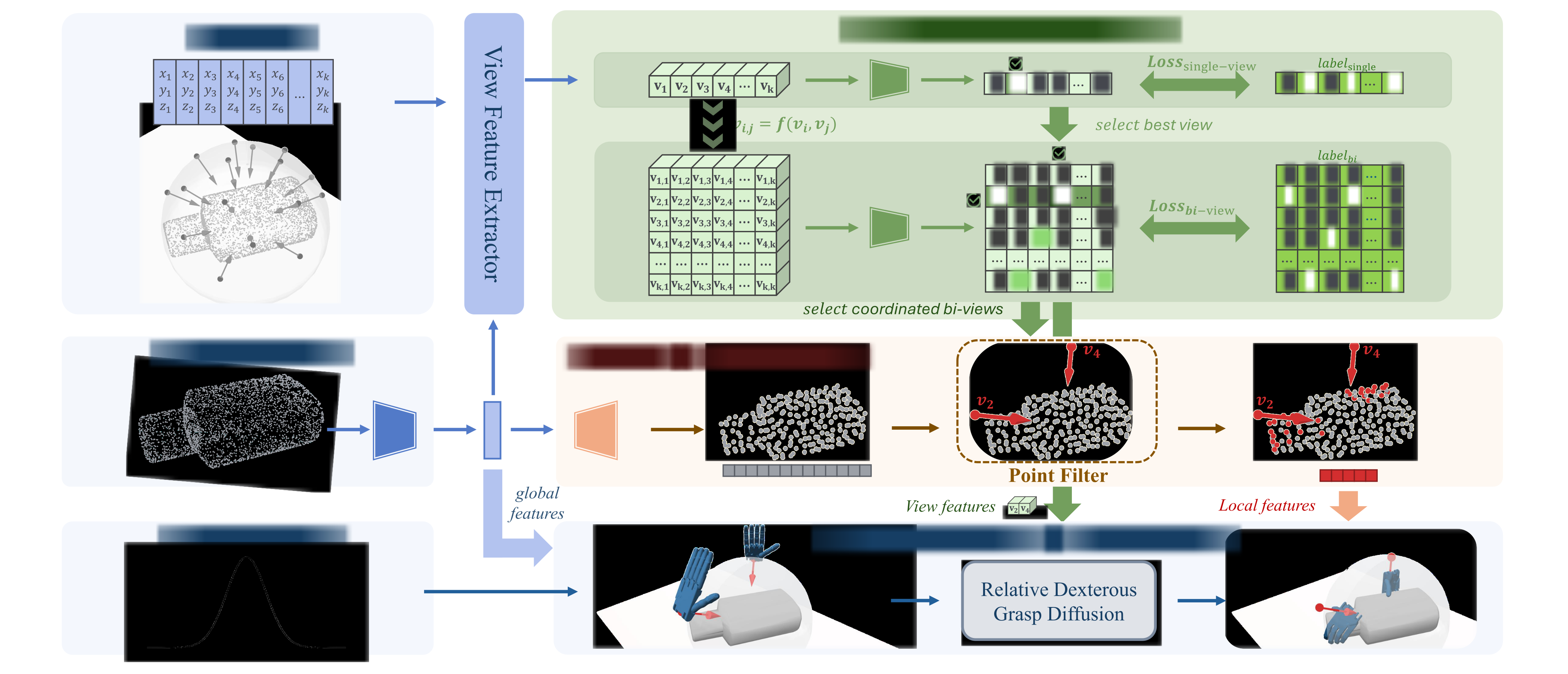
The learned model receives an object point cloud and outputs both wrist poses and finger configurations. A coordination module selects approach views; adaptive anchors and local geometry reduce the variation that the relative-pose diffusion model must explain.
5.1 Bimanual Coordination Module.
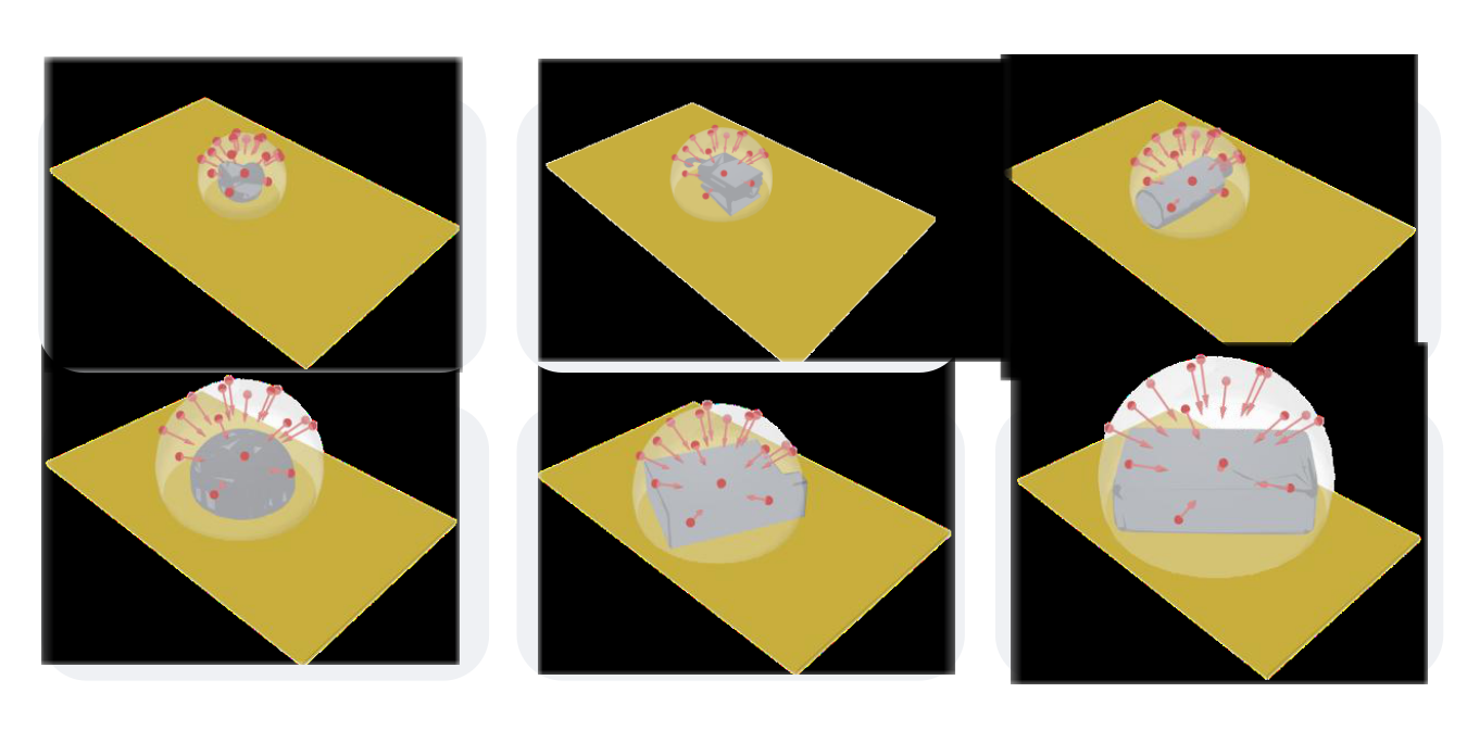
Cross-attend sixteen learnable view embeddings to PointNet++ object features. For each view pair, an MLP combines the two features, their difference and elementwise product to predict compatibility.
Supervise single-view and pairwise scores with SmoothL1 against normalized counts of successful training grasps assigned to their nearest candidate views. These are distributions induced by the synthetic dataset, not separately calibrated real-world success probabilities.
At inference choose a primary view and then a compatible secondary view. This conditional construction explicitly coordinates the two hands before continuous pose generation.
Equations
5.2 Geometry-Size-Adaptive Grasp Generation Strategy
Intersect each selected approach direction with the object’s minimum bounding sphere to obtain an anchor, then predict wrist translation/rotation relative to it (equation 2). The anchor removes much absolute scale variation while retaining fine pose offsets.
Use 256 representative object points and sixteen nearest neighbors around each anchor to extract local geometry; concatenate local, view and global features (equation 3). The source calls FPS “upsampling,” but FPS selects representative input points rather than synthesizing new surface samples.
DDPM generates relative bimanual wrist parameters and finger joints (equation 4). Training combines view regression, parameter L2, hand-surface Chamfer and physical penalties for penetration/contact (equation 5). Physical losses encourage feasible poses but do not enforce hard collision-free output.
Equations 2–3
| (2) |
| (3) |
| Method | SUC-F | SUC-L | SUC-A | S | PD | SPD | CDC | D |
| DexGraspNet | ||||||||
| BimanGrasp [28] | 26.80 | – | – | 0.16 | 1.52 | 0.26 | 1.87 | 0.150 |
| Ours(Float) | 75.84 | – | – | 6.73 | 0.17 | 0.02 | 0.59 | 0.190 |
| Ours(TableTop) | 77.11 | 80.83 | 71.34 | 6.87 | 0.15 | 0.02 | 0.52 | 0.165 |
| Objaverse | ||||||||
| BimanGrasp [28] | 30.21 | – | – | 0.16 | 0.87 | 0.23 | 1.38 | 0.156 |
| Ours(Float) | 70.82 | – | – | 4.55 | 0.20 | 0.04 | 0.67 | 0.180 |
| Ours(TableTop) | 62.41 | 70.41 | 62.40 | 5.10 | 0.20 | 0.05 | 0.67 | 0.158 |
Equations 4–5
| (4) |
| (5) |
6 Experiments
Experiments assess synthetic data quality, learned pose generation and real execution separately. Main comparisons and ablations use different training schedules and pose coverage.
6.1 Experiment Settings
MuJoCo evaluation uses Shadow Hand, friction coefficients 0.6/0.02, gravity 9.8 m/s² and the source’s stated object density of 2.5 kg/m³. That unusually low printed density is retained rather than silently converted; physical success depends on the simulated mass and friction assumptions.
The reported 12,000 synthesis instances imply 1,000 objects from each of two datasets at six sizes, with five candidates each: 60,000 grasps per method. BimanGrasp receives palm offsets of ±1 cm and finger perturbations of ±0.1 rad for pre-grasp/squeeze execution.
Learned generation uses the 2,397-object DexGraspNet tabletop subset, split by object 4:1, with 3,112,117 training grasps. Test three candidates per object pose/scale, totaling 139,956 grasps. This is narrower than evaluating all 6,351 dataset objects.
6.2 Implements Details
Synthesis weights QP/distance/region terms by 1,000/100/50. Dataset generation runs eight RTX 3090 GPUs, forty parallel worlds per GPU and twenty grasps per world.
Use sixteen views, 256 representative points and sixteen local neighbors. Comparison models train five epochs; ablations train twenty epochs on a subset with one tabletop pose per object and all scales. Framework experiments use one RTX 4090. These regimes explain why the ablation’s 61.9% is not directly interchangeable with the main 66.8% result.
6.3 Evaluation Metrics
SUC-F tests disturbance resistance, SUC-L tabletop lifting with floating hands and SUC-A lifting with arm control. S and SGS are raw and successful grasps per second. PD/SPD measure object-hand and intra-/inter-hand penetration; CDC measures spread in finger contact distances.
D is the first principal component’s explained variance ratio, so lower values indicate less concentration by this proxy. It is neither a direct count of grasp modes nor an independent measure of useful task diversity. Tables 3–5 preserve all synthesis, baseline and framework-ablation results.
6.4 Data Synthesis Experiments
On DexGraspNet, floating synthesis reaches SUC-F 75.84% versus BimanGrasp’s 26.80%, with 6.73 versus 0.16 grasps/s. Tabletop synthesis reaches 80.83% floating-hand lifting and 71.34% arm-controlled lifting. Objaverse results are lower but still exceed the floating baseline.
The raw reported speed ratios are about 42× for DexGraspNet and 28× for floating Objaverse. Appendix D says baseline speeds are copied from original reports, so these are not a controlled same-hardware timing comparison.
Adding region initialization, decoupled quality and pre-grasp strategy raises SUC-L 28.3→44.4→57.7→80.8% and SUC-A 12.9→39.8→49.5→71.3%. The sequential ablation supports their combined contribution without isolating all interactions.
6.5 Generation Framework Experiments
Table 4 compares the adapted SceneDiffuser and DGTR generators: SUC-L is 15.2%, 41.5% and 66.8% for BiDexGrasp. Its PD remains 1.53 cm, despite a much smaller SPD of 0.01 cm; generated poses are not perfectly penetration-free.
In Table 5, adding geometry/scale components alone raises success 41.2→44.7%; coordination plus local geometry gives 52.7%, and the full model gives 61.9%. Local features and anchors are not fully separated in every combination. The prose’s diversity trade-off is ambiguous: its defined lower-is-more-diverse D is 0.197 versus DGTR’s 0.201, but worse than SceneDiffuser’s 0.174.
6.6 Real-World Experiments
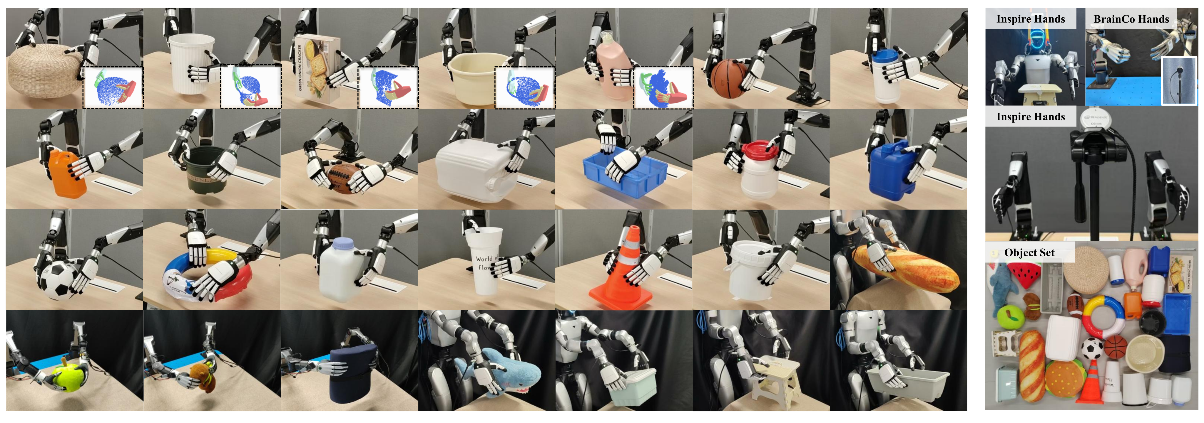
Execute 260 trials on thirty objects using Inspire/BrainCo hands and Unitree G1, Piper and Nero arm platforms. Single-view RGB-D uses Grounded-SAM segmentation; the “full cloud” condition samples a Hyper3D reconstructed mesh after scale alignment and FoundationPose pose estimation.
Reported success is 66.0% for the partial single-view input and 76.7% for the reconstructed full cloud, with 74.6% overall. Per-condition/platform trial counts and uncertainty intervals are not supplied, so the overall value should not be mistaken for their unweighted mean. Shadow Hand predictions are retargeted before execution.
7 Conclusion
The contribution is a broad synthetic bimanual pose dataset plus a view- and anchor-conditioned generator. Results support improved candidate quality and tested grasp execution, while leaving task-specific manipulation, heavier object assumptions and end-to-end arm-hand policy learning for further work.
8 Limitations
Fixed hand contact candidates limit contact-space diversity. Stability-oriented grasps need not satisfy functional requirements such as tool use. The network predicts floating-hand poses and does not use the dataset’s IK configurations to learn joint arm-hand outputs.
Additional evaluation limits include synthetic supervision, a narrower learned-model test subset, only thirty real objects, no reported real confidence intervals and residual penetration/noncontact failures. Generalization across the tested shapes/sizes does not establish robustness to arbitrary mass, friction, occlusion or semantic tasks.
Appendix A Preliminaries
Equation 6 retains the contact-force constraints and full 6×3 grasp matrix, mapping normal/tangent forces and their moment arms into object-frame wrenches. The normal force is bounded between zero and one; μ sets friction. The printed friction condition is conic, although the prose calls the cone discretized.
The individual wrench sets combine by Minkowski sum. Equation 7 optimizes contact forces to approximate each target disturbance, with a positive lower bound γ on total normal force and target scale β. The exact matrix, wrench-sum and feasible-set definitions are retained; numerical β/γ values and the complete disturbance-vector list are not given.
Equations 6–7
| (6) | ||||
| (7) | ||||
Appendix B Data Synthesis Details
The synthesis appendix specifies region separation, orientation/finger initialization and the nested optimization used to refine paired grasps.
B.1 Details of Bimanual Region-constraint Grasp Initialization
Keep a region pair only when its minimum point-to-point distance is at least 5 cm (equation 8). Choose palm orientation near preferred directions (1,−1,−1) for left and (1,1,−1) for right, supporting favorable arm configurations.
Normalize regional surface normals, average them and take resultant length R (equation 9). Angular variance V=2(1−R) below 0.005 marks a flat region (equation 10). Initialize fingers more open on flat surfaces and slightly curled otherwise. This heuristic depends on sampled normals and fixed thresholds.
Equations 8–10
| (8) |
| (9) |
| (10) |
B.2 Details of Decoupled Grasping Optimization
Equation 11 repeats the total constrained objective. Equation 12 sums squared contact-to-object distances. Equations 13–15 add a region penalty: zero inside distance a, a cubic Hermite transition until b=2a, then linear growth.
At fixed hand poses, solve the lower-level QP energies using ReLU-QP, an ADMM solver. Optimize hand parameters at the upper level using quality and geometric terms; cuRobo supplies joint-limit and collision energies. Numerical solver tolerances and region threshold a are not specified here. Penalty energies should not be read as a universal feasibility guarantee.
Equations 11–15
| (11) | ||||
| (12) |
| (13) |
| (14) |
| (15) |
Appendix C Framework Details
The framework appendix details candidate views, anchor coordinates, conditional sampling and every training loss.
C.1 Model Details
Sixteen candidate directions determine coarse approach geometry; the diffusion model then predicts continuous offsets and finger configurations around selected anchors.
C.1.1 Grasp View
Sample fixed unit directions on the upper hemisphere, pointing toward the object center. This tabletop-oriented restriction narrows the available approach family; it is not unconstrained full-sphere grasping.
C.1.2 Scale-Adaptive Grasp Anchor
Place the anchor at the chosen direction’s intersection with the minimum bounding sphere. Align its x-axis toward the center, project world z perpendicular to x for the anchor z-axis, and complete a right-handed frame.
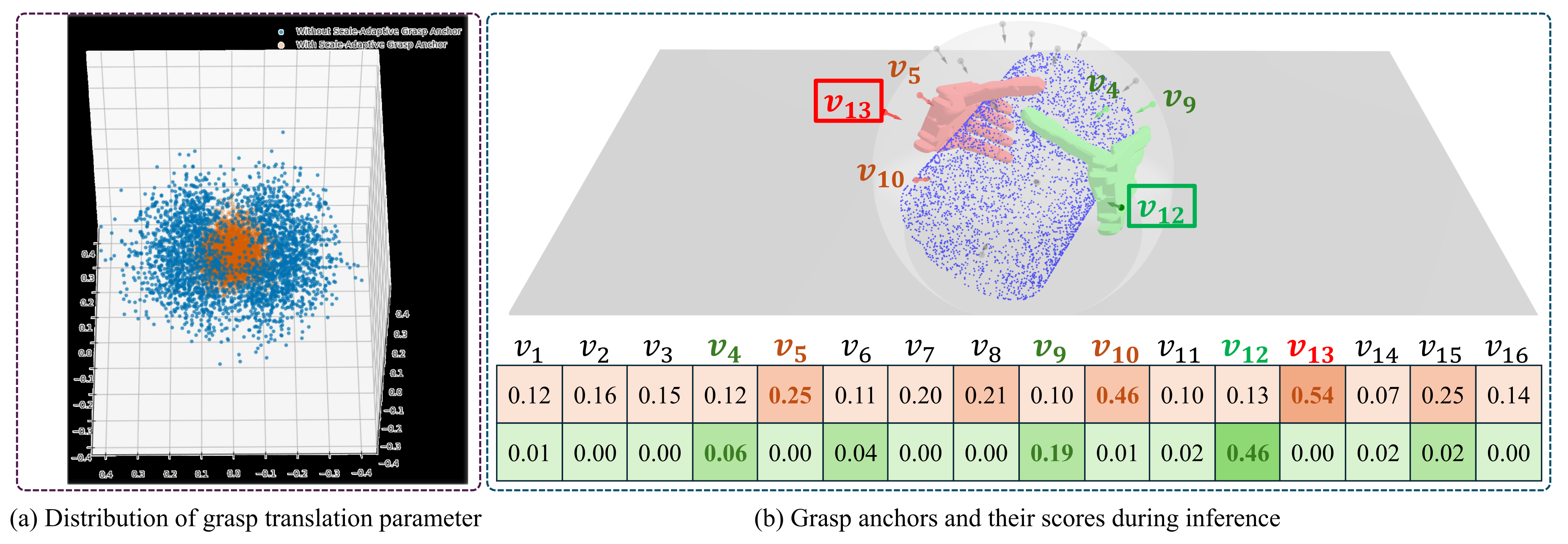
Translate/rotate world-frame grasps into this frame. Figure 6a shows more concentrated relative translations. The construction needs a fallback when approach x is parallel to world z; the source does not describe that degenerate case.
C.1.3 Selection of Grasp View in Training and Inference Time
Training uses ground-truth views to build anchors, a teacher-forcing choice that separates pose learning from predicted-view errors. Inference instead selects among the top five predicted primary views with softmax temperature 0.1, then applies the same strategy to the selected row of pairwise scores.
Figure 6b retains the example selecting primary view 13 and secondary view 12. This introduces a train/inference conditioning difference; the ablation tests sampling behavior but does not remove teacher forcing.
C.2 Loss Function Details
Equation 16 repeats the weighted objective. The following subsections retain each exact loss, mask and contact threshold definition.
Equation 16
| (16) |
Single-view Loss.
Equation 17 averages SmoothL1 primary-view score errors over valid supervised views, with ε preventing a zero normalization denominator.
Equation 17
| (17) |
Bi-view Loss.
Equation 18 applies SmoothL1 to every pair score but masks whole rows through the primary-view validity indicator. Normalize by valid rows times K, plus ε; there is no separately written validity mask for each secondary-view entry.
Equation 18
| (18) |
Parameter Loss.
Equation 19 penalizes squared L2 difference between predicted and ground-truth bimanual pose parameters. The text does not specify a separate rotation-manifold loss here.
Equation 19
| (19) |
Chamfer Loss.
Generate hand meshes from predicted and target poses, sample their surfaces and compute symmetric squared Chamfer distance (equation 20). This adds geometric supervision beyond parameter regression without requiring point-to-point mesh correspondence.
Equation 20
| (20) |
Physics-base Losses.
Equation 21 combines self-penetration, object penetration and contact-attraction terms. These differentiable penalties encourage plausible contact but do not replace execution validation.
Equation 21
| (21) |
Self-bi-penetration Loss.
Equation 22 penalizes pairs of predefined keypoints closer than safety threshold δ, covering both hands. Sparse keypoint separation is a proxy for continuous mesh collision, not an exact collision test.
Equation 22
| (22) |
Hand–Object Penetration Loss.
Equation 23 sums positive signed distances for hand keypoints inside the object. The source explicitly uses positive-inside convention; signs are retained unchanged.
Equation 23
| (23) |
Contact Loss.
Compute nearest object-surface distance for each contact candidate (equation 24) and average only candidates closer than τ (equation 25). Unlike the view losses, this expression has no written empty-set safeguard when no candidate qualifies.
Loss weights are single-view 10, pair-view 1, parameters 15, Chamfer 0.25 and total physics 1; within physics, object penetration is 100, self-penetration 50 and contact 50. Numerical δ/τ thresholds are not supplied here.
Equations 24–25
| (24) |
| (25) |
Appendix D Evaluation Metric Details
A simulated grasp succeeds when object translation/rotation remain within 5 cm/15° for at least three seconds after execution. Distinguish six-disturbance testing, floating-hand tabletop lift and arm-controlled lift; their denominators and mechanics are not interchangeable.
PD/SPD are maximum mesh penetration distances. CDC is the range of signed finger-contact distances. D is the first PCA component’s explained-variance ratio, inversely interpreted as diversity. S/SGS are raw/successful grasps per second on one RTX 3090 for this method; baseline timings are cited from prior reports.
Appendix E Experiments of Data Synthesis
Additional synthesis tests examine region ranking, clutter constraints, another hand model and visual diversity across scale.
E.1 Qualitative Experiments of Region Selection
Sample 2,000 objects from each mesh collection, five region pairs per object and five contacts per region. Table 6 reports Q1×10⁻² of 1.25 versus 0.47 on DexGraspNet and 1.41 versus 0.79 on Objaverse for ranked versus random regions.
These sampled contact-quality scores support better initialization; they are not measured physical success rates. The prose’s reference to Table 7 is stale; the region table is numbered 6.
| Method | ours(DGN) | random(DGN) | ours(Objaverse) | random(Objaverse) |
| Q1() | 1.25 | 0.47 | 1.41 | 0.79 |
E.2 Extension to Cluttered Scenes
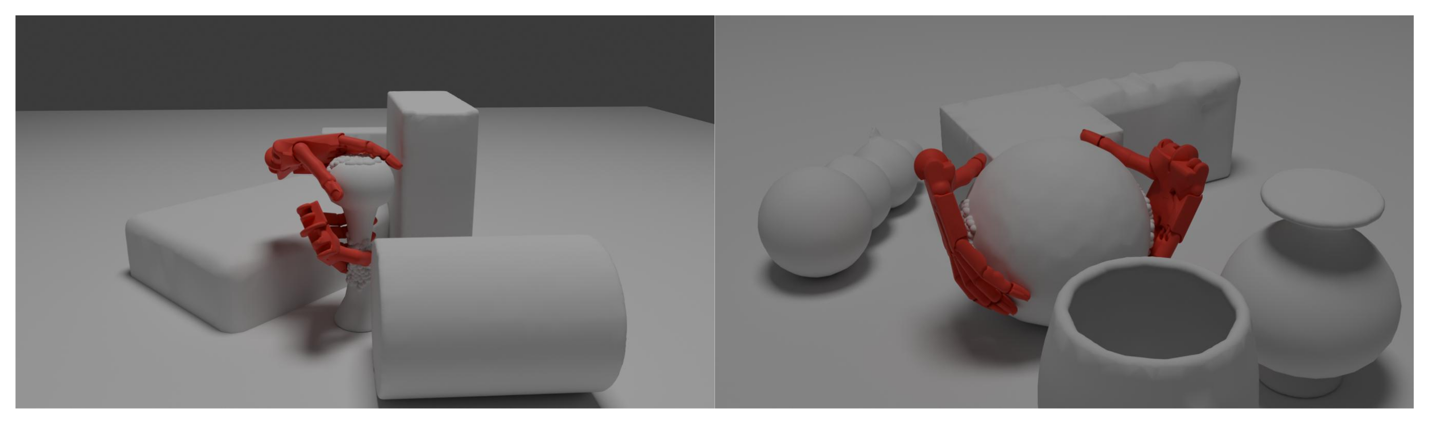
Figure 7 adds collision constraints for clutter and shows two examples. No quantitative clutter benchmark or end-to-end perception/planning success rate is reported for this extension.
E.3 More Visualization of Diverse Grasping on Data Generation
The following panels retain cross-hand synthesis examples and the dataset’s size/pose variation. Visual diversity is distinct from coverage of every possible stable or functional grasp.
E.3.1 Visualization of other Dexterous Hands
Figure 8 applies synthesis to LEAP Hand. It demonstrates that the optimization pipeline can be adapted to another embodiment; it does not establish zero-shot transfer of the learned Shadow Hand generator.

E.3.2 Visualization of Grasps in our Dataset
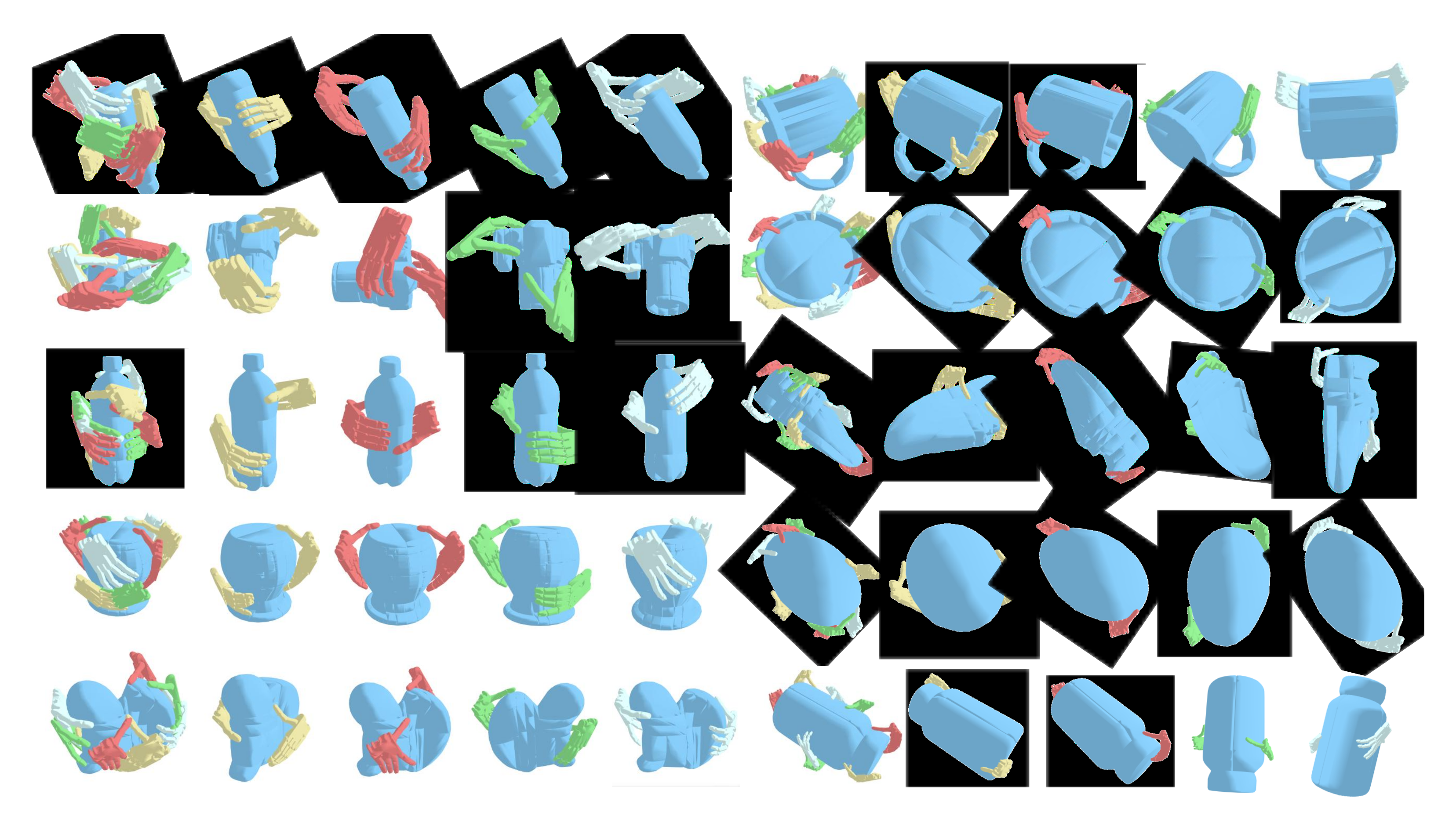
Figure 9 retains all grasp examples over multiple scales and object shapes, including alternative poses for the same tabletop placement. They illustrate the generated distribution rather than quantify its independent modes.
Appendix F Experiments of Framework
The framework supplement describes bimanual baseline adaptations, batch inference timing, conditional-view ablation and selected failure/success cases.
F.1 Reproduction of SOTA method
Adapt DGTR by doubling the output dimensions of its translation, rotation and joint MLP heads, summing the two hands’ losses and following its three-stage training procedure. Adapt SceneDiffuser by doubling input/output dimensions and retaining its existing loss.
These are bimanual adaptations of earlier methods, not native bimanual architectures with every component redesigned or independently tuned for this task.
F.2 Efficiency Analysis of Framework
At batch size 64, baseline inference is 1.21±0.03 s and BiDexGrasp 1.67±0.05 s: roughly 38% more batch latency, while SUC-L rises 41.17→61.93%. Measurements span five epochs.
This is batched model inference, not per-grasp robot execution latency or total sensing–retargeting–planning time. It is separate from synthesis throughput.
| Method | Average Inference Time (s) | Success Rate-Lift(%) |
| Baseline | 41.17 | |
| Ours | 61.93 |
F.3 Further Ablation of the Bimanual Coordination Module
Sampling a single pair directly from the pairwise score matrix yields 45.49% success versus 61.93% for primary-then-conditional sampling. PD improves 2.23→1.73 cm and CDC 2.96→2.56 cm, but SPD slightly worsens 0.01→0.02 cm.
This supports the implemented selection procedure. In probability theory a joint distribution can be factorized conditionally, so the result does not prove conditional sampling is intrinsically superior to every equivalent joint sampler; score normalization and top-k decisions matter.
F.4 Failure Case Analysis
Figure 10 retains penetration, noncontact and lateral-sliding failures. Competing contact and penetration losses can leave small geometric errors, while insufficient force closure can destabilize execution. No failure-category frequencies are provided.

F.5 More Visulization of Generated Poses
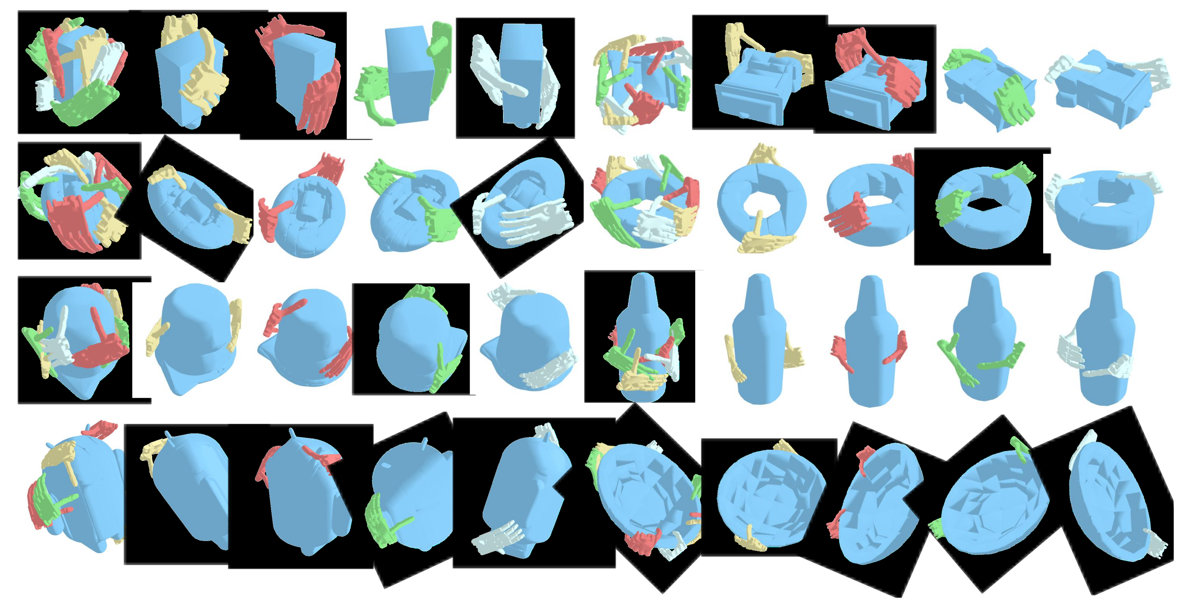
Figure 11 retains the full additional grid of model-generated bimanual grasps. The examples illustrate varied shapes, scales and paired poses; their selection does not establish a failure-free generation distribution.
Appendix G Real world Experiments
The real execution appendix specifies how object sensing, reconstructed geometry, hand retargeting and arm motion surround the learned floating-hand generator.
G.1 Real world Experiments Details
For partial input, segment a single RGB-D frame with Grounded-SAM. For “full” input, reconstruct a mesh from a single image, scale it by matching observed/reconstructed 3D bounding boxes, estimate its 6D pose, and sample the transformed mesh. The full cloud therefore includes generated hidden geometry, not an independently measured complete scan.
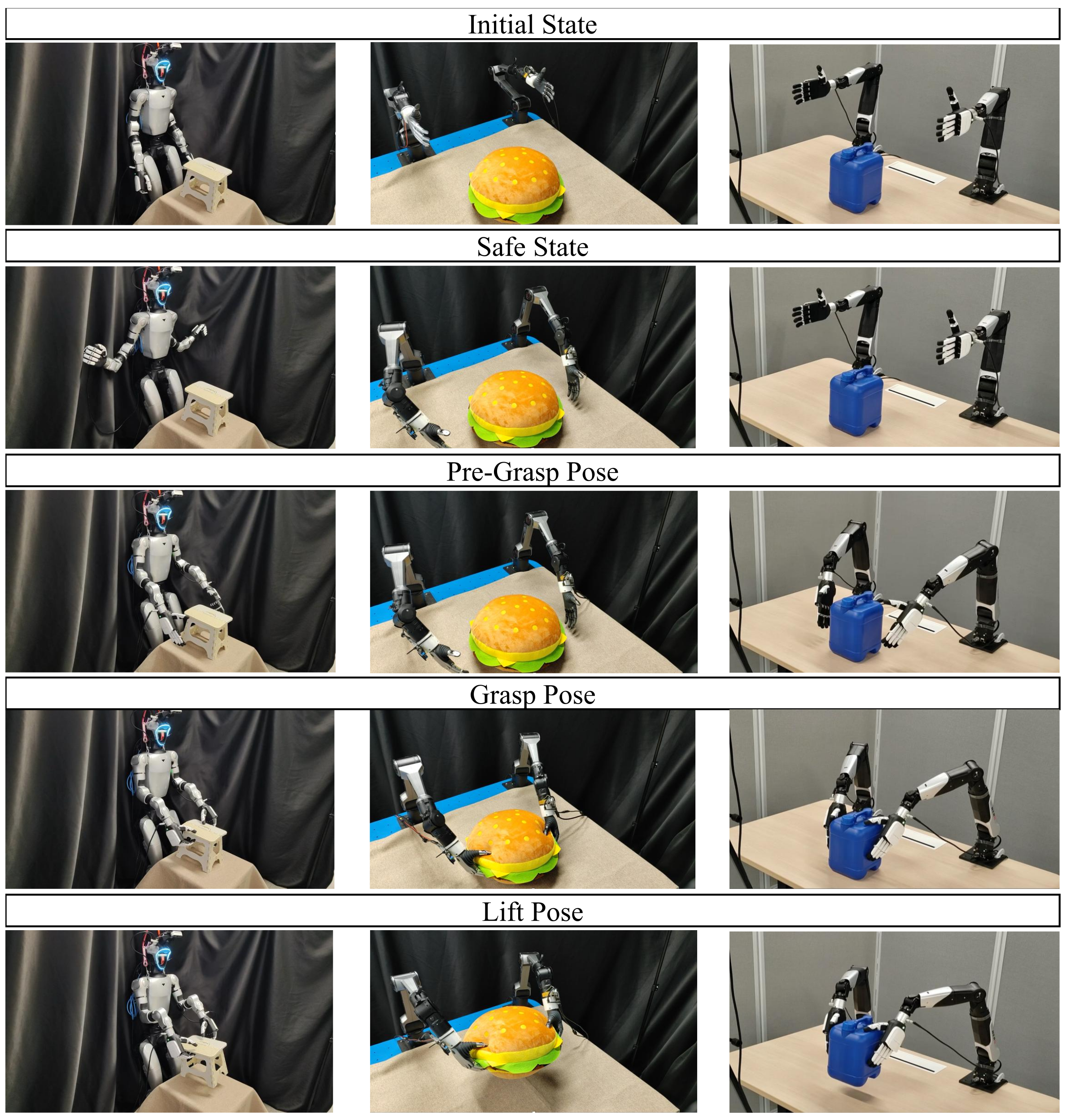
Retarget Shadow Hand joints with hand-object consistency; the appendix cites OmniDexGrasp while the main text cites Grasp as You Say. Retreat along each hand’s negative approach direction to form a pre-grasp, then execute safe configuration→pre-grasp→final grasp→lift. Figure 12 preserves all fifteen frames across three examples.
The real appendix does not specify a squeeze extrapolation identical to the synthetic protocol, the retreat distance, detailed per-platform trial counts or a separate physical success definition. These omissions limit exact reproduction of the aggregate real rate.