Overview
RAGEN-2 examines a failure of agent reinforcement learning: varied language can become insensitive to the particular problem. It pairs a cross-input diagnostic with reward-variance filtering and retains the full mathematical appendix.
At a glance
Reasoning can remain fluent and varied while converging to reusable templates across different inputs. RAGEN-2 diagnoses this with prompt–reasoning compatibility scores and proposes filtering updates toward prompts with informative reward differences. Results support the intervention across several agent tasks, algorithms and model sizes, with explicit exceptions when reward variance mainly reflects noise. The measurements are operational proxies for input dependence, rather than direct measurements of reasoning correctness or causal faithfulness.
1 Introduction
Ordinary reward and entropy monitoring can miss a policy that produces different-looking versions of the same generic rationale. Building on RAGEN, this work separates diversity within an input from differences across inputs. Its contribution is a diagnosis of template collapse, a gradient signal-to-noise interpretation, and an inexpensive update filter based on within-prompt reward variance. The empirical argument combines training curves, cross-run correlations and filtering interventions; the appendices state the assumptions behind the accompanying bounds.
2 Template Collapse in Multi-turn Agent RL
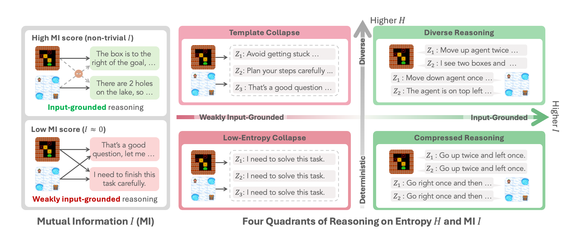
The proposed failure mode concerns the relationship between an input and its generated reasoning. A model may preserve token variability without preserving that relationship.
2.1 Setup and Preliminaries
At each interaction turn the agent sees an observation, produces reasoning and an executable action, and receives reward. The diagnostic input includes the complete available history; the measured reasoning excludes action tokens and boundary markers. Policy-gradient objectives combine reward-weighted updates with KL and entropy regularizers. These regularizers do not weight trajectories by reward differences, although their gradients can still depend on the prompt.
Equation
2.2 Rethinking Reasoning Collapse from an Information-Theoretic Lens
The entropy decomposition distinguishes within-input randomness from cross-input information. High values on both axes describe diverse, input-sensitive reasoning; high randomness with low input dependence describes template collapse. Low randomness can instead be either input-sensitive compression or complete collapse. Thus shorter or more deterministic reasoning alone does not establish that a model has stopped responding to its input.
Equation
2.3 Mutual Information Proxy Family
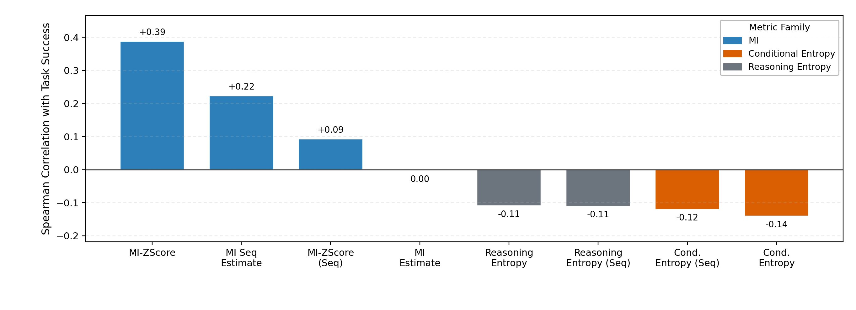
For each sampled reasoning trace, teacher-forced scoring compares its likelihood under its own prompt and every other prompt in the batch. Retrieval accuracy asks whether the original prompt ranks first; chance is 1/P. A continuous proxy compares matched likelihood with a uniform prompt-mixture likelihood, with per-token normalization and optional z-score/EMA smoothing. First-turn and trajectory-sampled variants are retained in Table 1. The reported strongest correlation with task performance is +0.39, while entropy correlations are −0.11 to −0.14. These scores depend on the scorer and candidate prompts; they are not exact Shannon MI. Reusing rollouts avoids additional sampling, but constructing the cross-score matrix still requires likelihood evaluations.
| Type | Proxy | Formula | Notes |
| Discrete | Retrieval-Acc | Chance level under template collapse | |
| bi lilin k | Recall@ | ||
| Continuous (raw) | MI-Est | Per-token; approaches 0 under collapse | |
| MI-Seq-Est | Per-sequence; no length normalization | ||
| Continuous (z-score) | MI-ZScore | Normalized by current-batch marginal std | |
| MI-ZScore-EMA |
Equations 1
| (1) |
3 The Mechanism of Template Collapse: A Signal-to-Noise Ratio (SNR) View
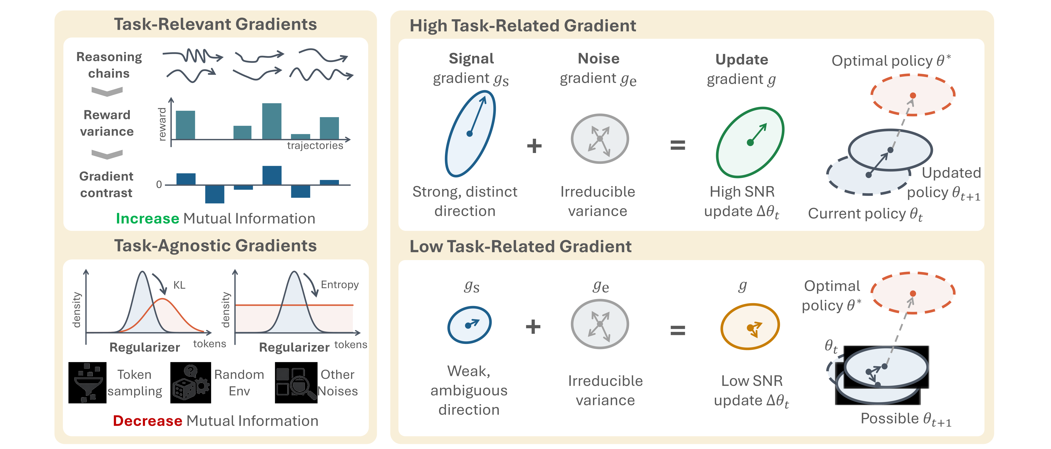
The proposed mechanism is an imbalance between reward-discriminative gradients and other update components. When rewards barely distinguish trajectories for a prompt, regularization and sampling noise can have greater relative influence. This motivates selecting update data by reward variation rather than regulating output entropy alone.
3.1 Observing Signal-Noise Imbalance in RL Gradients
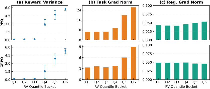
Figure 3 groups prompts into six reward-variance buckets for PPO and GRPO. Task-gradient norms increase with variance, while regularizer norms vary much less. The authors interpret this as weak task signal in low-variance groups. The caption also notes substantial low-variance task gradients, so the observation should not be reduced to a claim that every sampled gradient vanishes or that norm alone measures useful signal.
3.2 Formalizing the SNR Mechanism via Gradient Decomposition
With a conditional-mean baseline, Cauchy–Schwarz bounds the expected task-gradient norm by the square root of reward variance times a score-function factor. The update is then conceptually decomposed into task signal, task noise and regularization. This supports a low-variance weakness argument under the stated assumptions; it does not establish that high variance guarantees useful signal or that regularizers universally force MI to zero. Appendices H and K make the magnitude and dominance claims more precise.
Equations
| Component | Source | Level | Ctrl. | Mitigation |
| Meaningful reward differences across same-prompt trajectories | Prompt | No | SNR-Aware Filtering | |
| Sampling and environment stochasticity | Prompt | No | Filter high-noise prompts | |
| Uniform contraction per chain, independent of input (KL, entropy) | Chain | Yes | Tune , |

3.3 SNR-Aware Filtering: Prioritizing High-Signal Updates
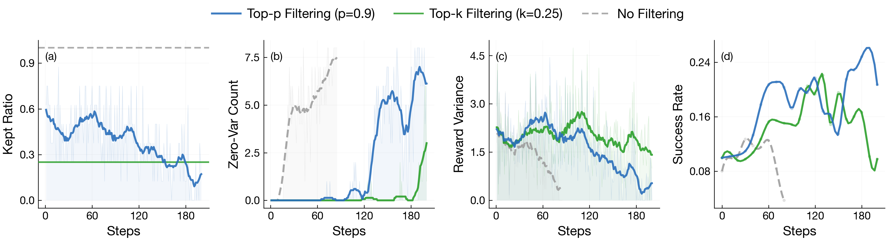
Sample several trajectories per prompt, estimate their return variance, and sort prompt groups from highest to lowest variance. Top-p filtering retains the smallest prefix containing a chosen fraction of total variance mass, then updates only on those groups. A setting of 0.9 therefore targets 90% of variance mass, not necessarily 90% of prompts. Selection happens after rollout collection, so it changes gradient contributions without changing that iteration’s sampling distribution. The score is cheap but conflates task-dependent variation with environmental or evaluation noise.
Equations
| Task | Stochastic | Multi-turn | State | Reward |
| Sokoban | ✗ | ✓ | Grid | Dense |
| FrozenLake | ✓ | ✓ | Grid | Binary |
| MetaMathQA | ✗ | ✓ | Text | Dense |
| Countdown | ✗ | ✗ | Text | Binary |
| SearchQA | ✗ | ✓ | Text | Dense |
| WebShop | ✗ | ✓ | Text | Dense |
| DeepCoder | ✗ | ✗ | Text | Dense |
4 Experiments
Experiments first examine collapse diagnostics, then compare filtering strategies, model/algorithm variants and interventions intended to probe the proposed mechanism. Reported peak validation performance should be distinguished from final-checkpoint performance.
4.1 Experimental Testbed
The testbed combines grid planning, navigation, mathematics, search, shopping and programming. Most controlled algorithm/model comparisons use four core tasks; additional plots cover search, web interaction and code generation.
Environments and tasks.
Sokoban stresses irreversible box pushes; FrozenLake adds sparse rewards and stochastic transitions. MetaMathQA tests mathematical answers, and Countdown constructs arithmetic expressions. SearchQA requires iterative retrieval, WebShop requires selecting products that satisfy instructions, and DeepCoder rewards executable solutions against tests. These tasks differ in observability, horizon and reward structure, so a shared filtering rule need not have the same effect everywhere.
Training and evaluation setup.
The main setup uses Qwen2.5-3B with veRL/HybridFlow and PPO, DAPO, GRPO or Dr. GRPO, for up to 400 iterations. A default iteration collects 128 trajectories as eight prompts with sixteen samples each. Filtering reduces the update batch, and the paper scales loss by the keep-rate parameter to keep step sizes comparable. Appendix B specifies validation, optimization and early stopping.
4.2 Template Collapse as a Consistent Failure Mode
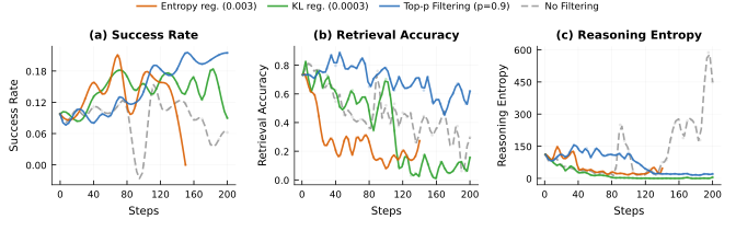
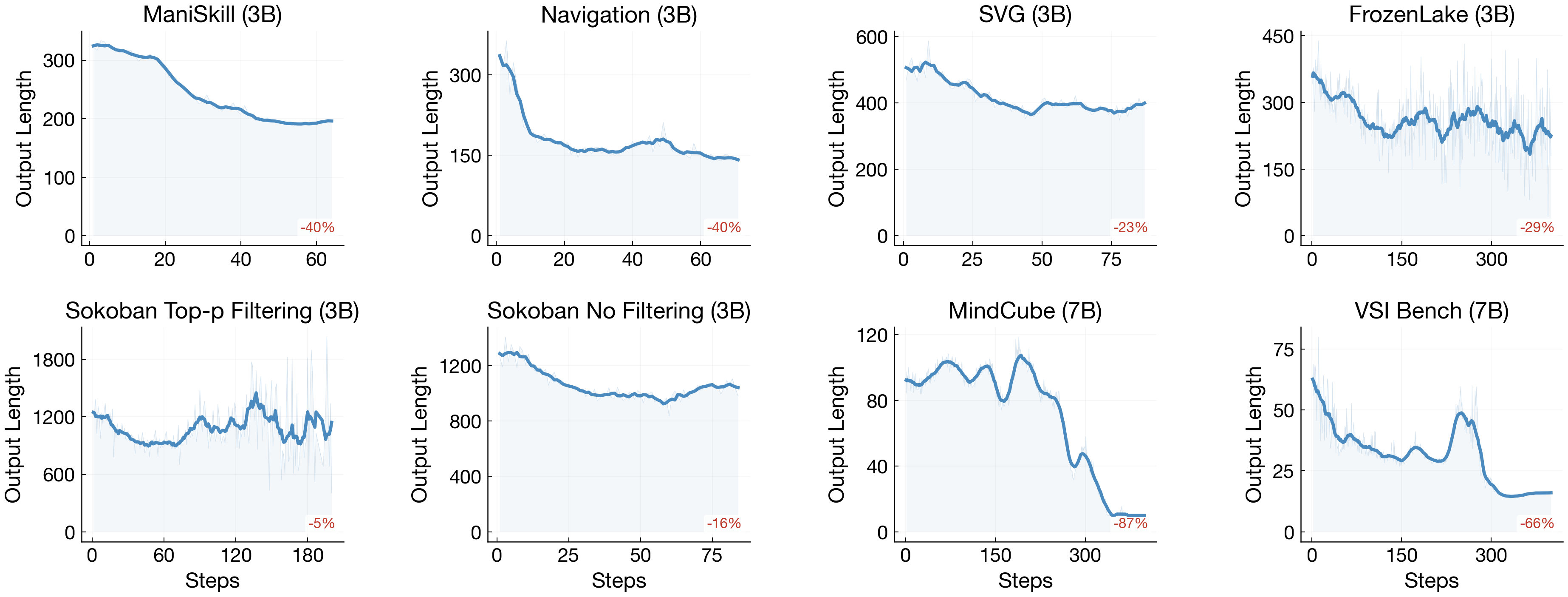
In the illustrated unfiltered runs, retrieval-based input dependence falls before task performance while reasoning entropy remains high or spikes. Filtering better preserves the diagnostic and task success. Additional length plots show compression in several settings, but length itself cannot distinguish efficient input-sensitive reasoning from generic templates; the input-dependence measurement is the central evidence.
| Experiment Variants | Sokoban | FrozenLake | MetaMathQA | Countdown | Average |
| Baseline | |||||
| PPO (Schulman et al., 2017b), | |||||
| Qwen2.5-3B (Qwen Team, 2024) | 12.9 (+16.0) | 67.0 (+10.9) | 92.6 (+0.6) | 97.9 (+0.0) | 67.6 (+6.9) |
| Algorithm | |||||
| DAPO (Yu et al., 2025) | 16.2 (+5.1) | 66.8 (+2.1) | 90.8 (+2.8) | 95.7 (+1.6) | 67.4 (+2.9) |
| GRPO (Shao et al., 2024) | 12.1 (+9.0) | 70.9 (-3.0) | 91.2 (+1.2) | 95.7 (+2.2) | 67.5 (+3.7) |
| Dr. GRPO (Liu et al., 2025) | 12.1 (-0.4) | 23.2 (+0.6) | 91.2 (+1.4) | 96.5 (+1.4) | 55.8 (+0.8) |
| Model Scale (PPO) | |||||
| Qwen2.5-0.5B (Qwen Team, 2024) | 3.3 (+22.9) | 19.5 (+0.0) | 10.0 (-0.2) | 23.0 (-0.7) | 14.0 (+5.5) |
| Qwen2.5-1.5B (Qwen Team, 2024) | 17.0 (+6.2) | 36.5 (+1.6) | 80.3 (+7.0) | 56.6 (+1.6) | 47.6 (+4.1) |
| Qwen2.5-7B (Qwen Team, 2024) | 42.4 (+4.9) | 85.0 (-0.6) | 84.0 (+11.7) | 97.7 (+0.3) | 77.3 (+4.1) |
| Model Type | |||||
| Qwen2.5-3B-Instruct (Qwen Team, 2024) | 22.5 (+14.2) | 83.6 (+2.3) | 91.2 (+0.4) | 96.3 (-0.6) | 73.4 (+4.1) |
| Llama3.2-3B (Meta Llama, 2024) | 24.4 (+18.8) | 84.6 (-0.2) | 86.1 (+3.7) | 99.2 (-1.2) | 73.6 (+5.3) |
| Modality (Input Type) | |||||
| Qwen2.5-VL-3B (T) (Bai et al., 2025) | 53.0 (+6.0) | 16.0 (+53.5) | - | - | 34.5 (+29.8) |
| Qwen2.5-VL-3B (V) (Bai et al., 2025) | 65.0 (+12.0) | 19.5 (+59.5) | - | - | 42.3 (+35.8) |
4.3 SNR-Aware Filtering Consistently Improves Performance
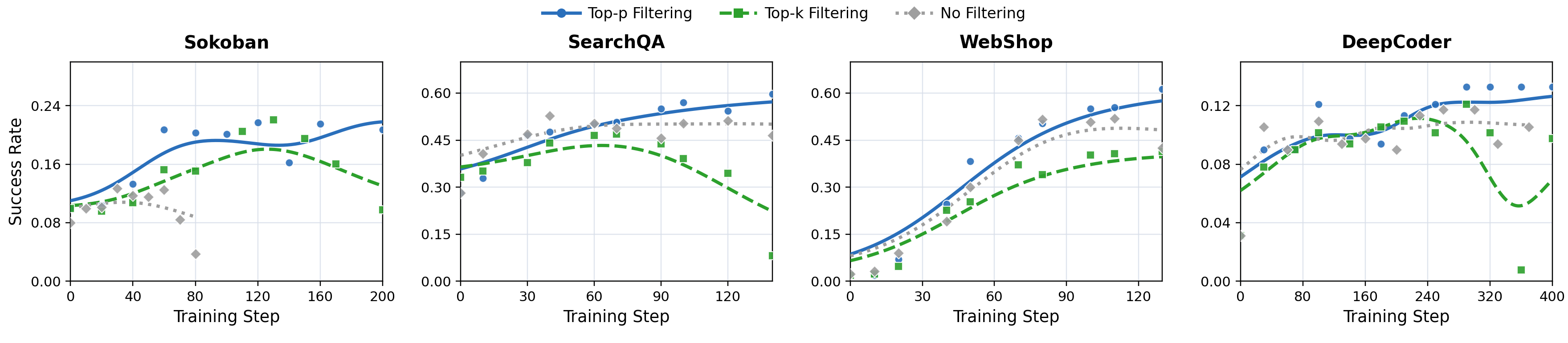
Table 4 reports higher average peak performance for every listed model/algorithm configuration, with individual task exceptions. Qwen2.5-3B PPO rises from 67.6% average by 6.9 percentage points; Sokoban rises from 12.9% by 16.0 points. Some cells decline, including Dr. GRPO on Sokoban and Qwen2.5-7B on FrozenLake. Figure 6’s actual panels cover Sokoban, SearchQA, WebShop and DeepCoder. At a fixed 128-rollout budget, Table 5 reports 26–41% shorter filtered update steps and under 0.1% overhead for variance calculation. This measures filtering cost, not the full cost of every MI cross-scoring diagnostic.
5 Analysis
The analysis asks whether the diagnostic separates interventions and whether controlled selection/noise experiments support the proposed signal-quality explanation.
5.1 MI Diagnoses Collapse Better Than Entropy Across All Interventions
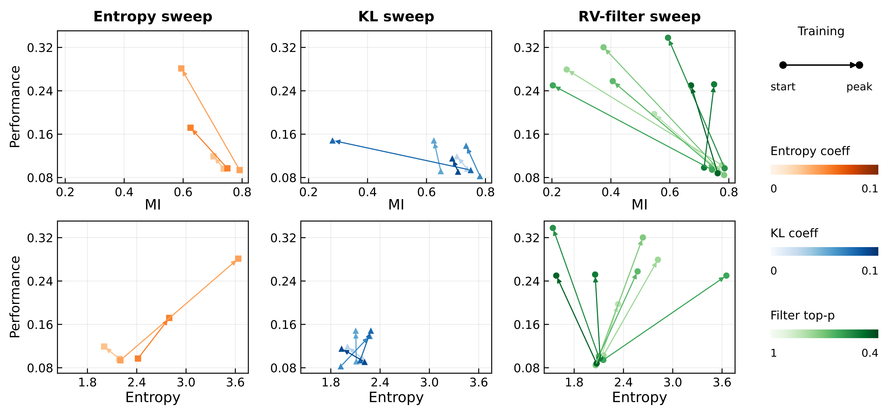
Entropy-strength, KL-strength and filter-mass sweeps trace different trajectories in performance–diagnostic space. The strongest reported MI-family correlation is +0.39; some MI variants are weaker or near zero, while entropy measures are slightly negative. This favors the selected proxy within these runs, without making it a universally calibrated predictor or validating the paper’s informal “twice as reliable” phrasing. KL anchoring can preserve properties of a reference policy without improving them.
5.2 Does SNR Mechanism Really Interpret Agent RL?
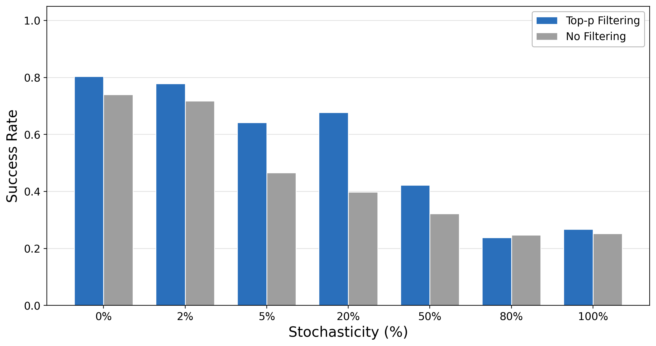
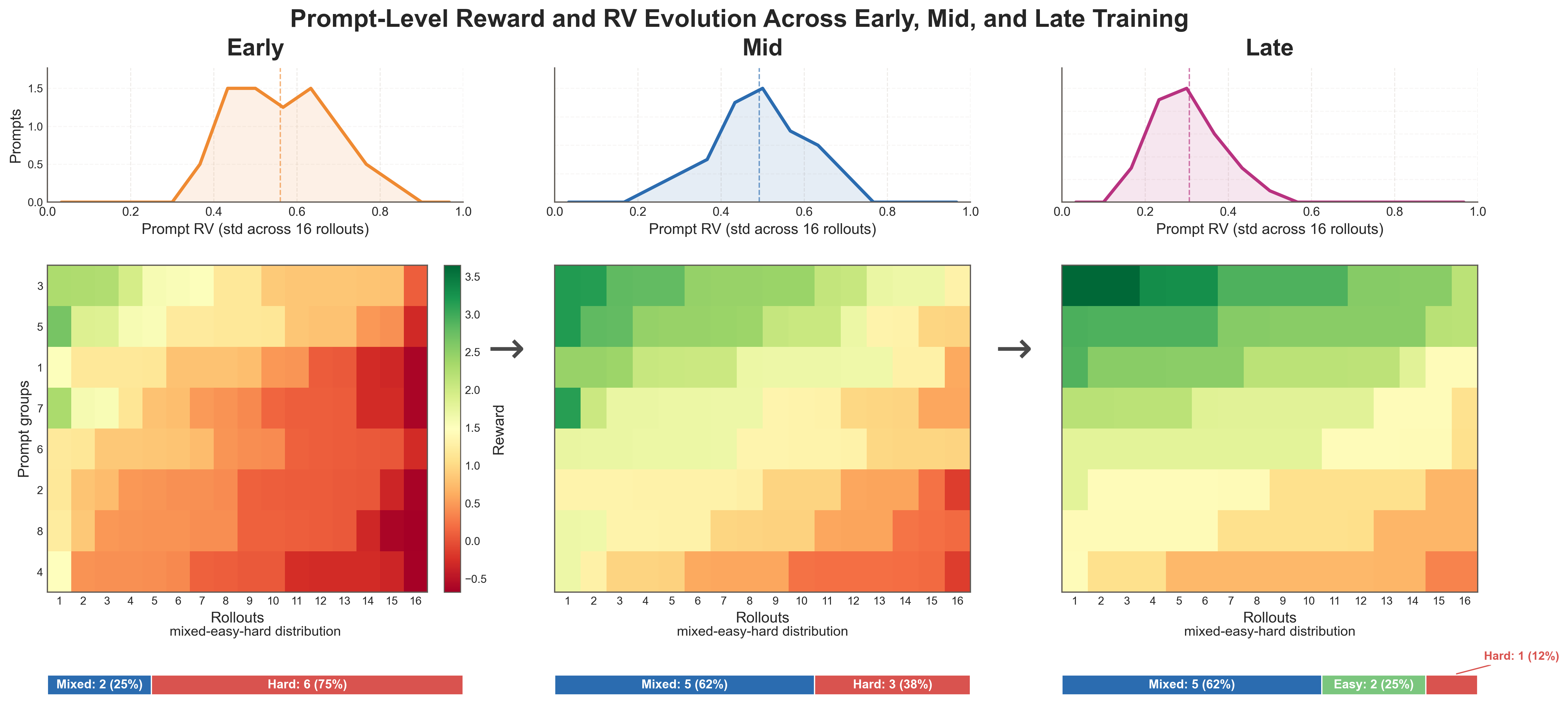
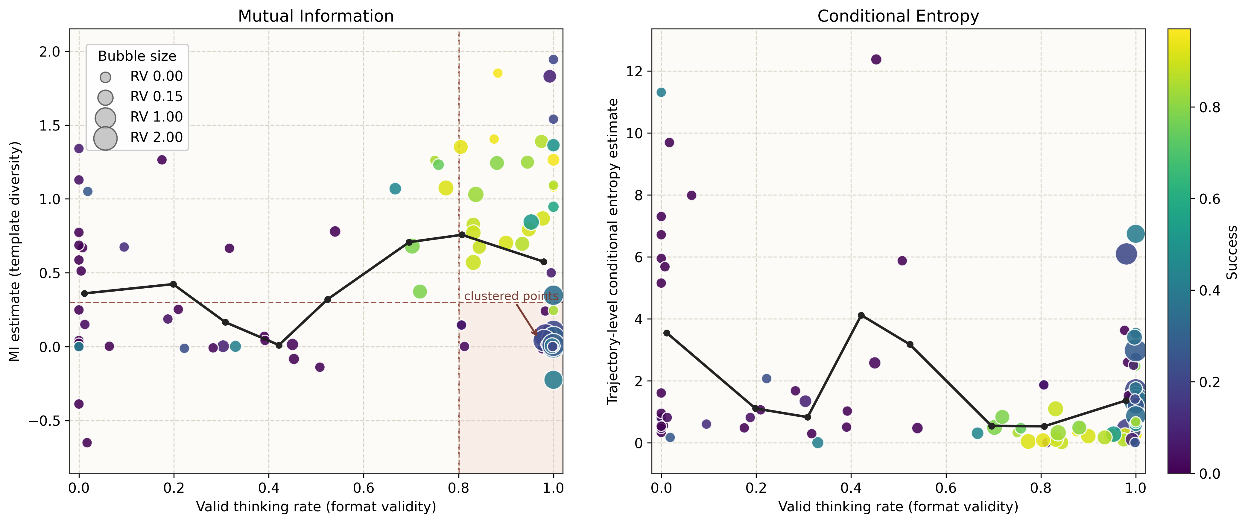
Keeping only the highest reward-variance quartile yields 21.1% Sokoban success versus 11.0% for the lowest; the intermediate task scores are not strictly monotone. In FrozenLake the filtering advantage largely disappears at 80–100% transition noise. A prompt-level filter reaches 23.6% versus 12.9% without filtering and 16.8% for the trajectory-selection baseline. The source’s trajectory counts and MI-proxy units are not fully consistent, so these results support an intervention effect without resolving every causal alternative. Cross-prompt variance heterogeneity also matters: Table 8 reports a −5-point FrozenLake GRPO case when variance is relatively uniform. As more prompts yield nearly identical rewards, adaptive selection tightens. High format validity can coexist with low input dependence; neither formatting, entropy nor response length substitutes for a content-sensitive diagnostic.
| Quartile | RV Range | Task Perf (%) | MI Proxy | Entropy |
| Q1 (highest RV) | [4.4–5.6] | 21.1 | 0.95 | 2.02 |
| Q2 | [1.5–4.2] | 19.5 | 0.93 | 1.53 |
| Q3 | [0.0–0.2] | 10.7 | 0.81 | 1.41 |
| Q4 (lowest RV) | [0.0–0.1] | 11.0 | 0.73 | 1.87 |
| Method | Prompts Used | Traj/Update | Task Perf (%) | MI Proxy |
| No filter | 8/8 | 128 | 12.9 | 0.83 |
| Prompt-level RV () | 3.2/8 | 50.6 | 23.6 | 1.80 |
| Trajectory-level | 8/8 | 64 | 16.8 | 0.20 |
6 Related Work
Related work distinguishes language-level rationale degeneration, action-policy concentration and collapse under repeated self-training. Lexical or embedding diversity does not necessarily measure whether differences follow the input. Retrieval-style matching probes that relationship, whereas reasoning faithfulness asks whether a rationale causally supports the decision. Filtering complements standard stabilization and credit-assignment methods by changing which sampled groups contribute updates.
7 Conclusions and Limitations
The practical takeaway is to monitor input dependence alongside reward and entropy, and to test whether reward-variance filtering improves a particular training regime. Limitations include coupling between task and regularizer gradients, single-agent experiments, possible gaming of the variance criterion, sparse/noisy rewards, reduced exploration under aggressive filtering, and task-dependent keep-mass tuning. The theoretical upper bounds and empirical proxies explain specific risks; they do not guarantee that retained reasoning is correct or faithful.
8 Acknowledgements
The authors acknowledge Yuxiang Lin for infrastructure and environment support, and Kyunghyun Cho for manuscript discussions.
Appendix Contents
The appendices provide extended context, experimental settings, diagnostic plots, filtering definitions and mathematical derivations. All original displayed formulas are retained below.
Appendix A Extended Related Work
The extended review separates three questions: what degenerates during closed-loop training, how to measure input-sensitive reasoning, and how stabilization methods interact with weak reward signals.
Reasoning collapse and policy degeneracy in closed-loop LM and agent RL training.
Repeated optimization on self-generated trajectories can narrow both language patterns and behavioral choices. Rationale templating may appear while external behavior still earns reward, so language-level collapse and policy-level degeneration need not coincide. Multi-turn interaction adds opportunities for cross-task templates and mechanical later-turn behavior.
Evaluating reasoning diversity, input dependence, and reasoning faithfulness.
Lexical overlap, distributional distance and token uncertainty measure output variation but may miss input-independent templates. Prompt reconstruction and matching provide a different diagnostic axis. Input sensitivity remains distinct from causal faithfulness: a rationale can mention the correct input without being the mechanism that produced the action.
Stabilizing multi-turn Agent RL under closed-loop sampling.
KL control, entropy bonuses, clipping, reward shaping, curricula, replay and intermediate supervision address related stability problems. When trajectories receive indistinguishable rewards, these mechanisms may still leave little directional task signal. The proposed filter acts on that data-selection problem and can coexist with those other controls.
Appendix B Detailed Experimental Settings
The experimental details specify reward functions, horizons, optimization and stopping rules. Several descriptions differ across sections, so those discrepancies are noted rather than silently harmonized.
B.1 Environments and Tasks
Sokoban gives +1 for placing a box, −1 for removing it, +10 for completion and −0.1 per action. FrozenLake’s stated default executes intended actions with 98% probability and rewards only reaching the goal. MetaMathQA describes exact-match correctness with halved reward after each retry; Countdown distinguishes correct, well-formed incorrect and malformed expressions. DeepCoder uses test outcomes, SearchQA rewards answers/search efficiency, and WebShop scores instruction–product matching. The appendix’s numerical Countdown example reuses a number despite the stated once-only rule; the notes retain the rule without adopting that example.
B.2 Training and Evaluation Setup
Interactive grid tasks use up to five turns with two actions each. This setup section assigns one turn to both Countdown and MetaMathQA, despite the earlier description of MetaMathQA retries. Actor/critic learning rates are 10⁻⁶/10⁻⁵, update batch size is 32, per-GPU minibatch size four, and entropy coefficient 0.001; malformed output incurs −0.1. Early stopping triggers after five persistently low-variance iterations or five validation checkpoints below 1% success. Evaluation uses 512 fixed prompts and temperature 0.5. The formal top-p rule is cumulative variance mass despite this section’s loose description as a prompt fraction.
Appendix C Filtering Ablation Results
Sokoban ablations vary token sampling, filter metric and retained variance direction. Table 9 reports peak success with diagnostics at that checkpoint, plus whether training ever collapses below 1% validation success. Reward-variance selection improves success from 0.17 to 0.38 in its comparison block; retaining the largest rather than smallest variance groups gives 0.44 versus 0.29 in a separate block. Entropy- and length-based alternatives can preserve one diagnostic while failing on stability or task success. Sampling parameters and filtering interact, so rows from different blocks do not form one controlled ranking.
| EXPERIMENT SETUP | TASK PERF | MI PROXY | ENTROPY | STABLE |
| Sampling Strategies | ||||
| Top-p = 1.0 (Baseline) | 0.17 | 0.54 | 2.76 | ✗ |
| Top-p = 0.9 | 0.38 (+0.20) | 0.84 (+0.29) | 1.64 (-1.12) | ✓ |
| Top-p = 0.5 | 0.29 (+0.12) | 0.83 (+0.29) | 1.88 (-0.88) | ✓ |
| Min-p = 0.05 | 0.42 (+0.25) | 0.67 (+0.13) | 1.64 (-1.12) | ✓ |
| Min-p = 0.2 | 0.45 (+0.27) | 0.36 (-0.18) | 3.01 (+0.26) | ✓ |
| Top-k = 0.25 | 0.22 (+0.05) | 0.86 (+0.32) | 1.28 (-1.48) | ✓ |
| Top-k = 0.5 | 0.44 (+0.27) | 0.89 (+0.35) | 1.47 (-1.29) | ✓ |
| Filtering Metrics | ||||
| No Filter (Baseline) | 0.17 | 0.54 | 2.76 | ✗ |
| Reward Variance | 0.38 (+0.20) | 0.84 (+0.29) | 1.64 (-1.12) | ✓ |
| Reward Sum | 0.24 (+0.07) | 0.80 (+0.26) | 4.18 (+1.42) | ✗ |
| Entropy | 0.20 (+0.02) | 0.41 (-0.14) | 2.20 (-0.56) | ✗ |
| Entropy Variance | 0.23 (+0.06) | 0.70 (+0.16) | 2.94 (+0.18) | ✗ |
| Length | 0.16 (-0.02) | 0.91 (+0.36) | 1.65 (-1.10) | ✗ |
| Keep Strategies | ||||
| Keep Largest (Baseline) | 0.44 | 0.89 | 1.47 | ✓ |
| Keep Smallest | 0.29 (-0.15) | 0.47 (-0.42) | 5.31 (+3.84) | ✓ |
Appendix D Additional Experimental Visualizations
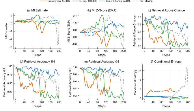
The supplementary plots show how several cross-scoring diagnostics and conditional entropy evolve under the same interventions.
D.1 MI Proxy Metrics During Training
Figure 14 includes the raw MI estimate, normalized/smoothed score, above-chance retrieval and retrieval at different candidate counts. The curves support the distinction between input dependence and entropy, with top-p filtering generally retaining stronger retrieval. The original trajectories are retained because individual metrics and regularization settings do not behave identically.
Appendix E Notation and basic identities
The notation distinguishes the policy’s true distribution from the fixed-scorer quantities used to approximate it.
E.1 Random variables and distributions
A rollout consists of a prompt, sampled reasoning trajectory and reward. Subtracting the conditional mean reward yields a within-prompt zero-mean advantage; the policy score is the gradient of log likelihood and has zero expectation under regularity conditions. Reward variance measures observed spread, which may come from meaningful trajectory differences or evaluation noise.
Equations
E.2 Entropy and mutual information
Conditional entropy measures average variability for a fixed input. Mutual information measures how far each conditional reasoning distribution differs from the marginal distribution over reasoning. These are properties of the full policy-induced distribution.
Equations
Decomposition identity (Shannon quantities).
The Shannon identity relates true marginal entropy, conditional entropy and MI. Scorer-defined likelihood quantities are measured under a possibly different distribution and need not equal these Shannon quantities. Their diagnostic interpretation depends on how well the scorer represents the evaluated policy.
Equations 2
| (2) |
Interpretation for reasoning diversity.
A fall in conditional entropy means greater within-prompt concentration; a fall in MI means weaker cross-prompt discrimination. Tracking both prevents treating all compression as the same failure mode. Low reward variance is one proposed condition under which reward-agnostic updates gain influence.
Appendix F Scorer-based Proxies for Reasoning Diversity
This appendix formalizes matched and mixture likelihoods using a fixed scorer and a sampled collection of prompt groups.
F.1 Setup and notation
For each of P prompts, sample G trajectories and score every trajectory under every prompt. The matched score uses the originating prompt; the mixture uses a log-sum-exp over the uniform prompt set. Both depend on the scorer and batch composition. Appendix F fixes the scorer, whereas the main description writes current-policy likelihoods; the paper does not fully reconcile those conventions. Neither finite-batch proxy should be treated as exact MI without additional assumptions.
Equations
Appendix G Formal Definition of the Filtering Operator
A filter is specified by a grouping key, a statistic computed within each group, and a selection mask. Multiplying the per-sample loss by that mask removes rejected groups from gradient computation. The displayed definition is general; reward variance and prompt grouping are the paper’s primary instantiation.
Equations
Remark (post-sampling).
Filtering occurs after sampling. It leaves the already-collected rollout distribution intact while changing the distribution of samples used for optimization.
Remark (normalization).
Normalizing by all samples, retained samples or retained groups changes gradient scale even when the selection mask is identical. This is relevant when comparing learning rates and effective batch sizes.
G.1 Filtering Strategy Variants
The variants share prompt groups and return-variance scores; their difference is how the kept subset is selected.
Top-p (nucleus-style) filtering.
Top-p sorts by descending variance and keeps the smallest prefix reaching a chosen share of total variance mass. The number of groups adapts to the distribution. Zero-signal batch rejection requires the implementation’s handling of zero groups and numerical thresholds; it does not follow automatically from the positive-total-mass formula alone.
Equation
Top-k (proportional) filtering.
Top-k retains a fixed fraction of groups by rank. It controls update count directly but can retain weak groups when little useful variation exists anywhere in the batch.
Equation
Min-p (threshold) filtering.
Min-p keeps groups whose variance exceeds a chosen fraction of the maximum. It adapts the count to a relative quality threshold, but a fluctuating maximum can make selection unstable.
Equations
Reverse top-p (low-variance) filtering.
Reverse top-p prioritizes low-variance groups as a diagnostic intervention. Its role is to test whether the high-variance direction matters, rather than merely reducing the update batch.
Implementation notes.
The implementation can exclude exactly zero-variance groups before selection and uses epsilon 0.01 for cumulative-threshold checks. These details affect degenerate batches and are separate from the idealized operator.
Appendix H RV Controls Task-Signal Magnitude and SNR
The bounds connect observed reward variation to expected task-gradient magnitude and sampling noise under explicit assumptions. They provide upper bounds and illustrative cases, not a guarantee that high-variance prompts carry useful gradients.
H.1 Setup
Fix a prompt and sample trajectories from its conditional policy. Use the conditional mean reward as baseline, so the second moment of advantage equals reward variance. The score-function norm supplies the additional factor in the gradient bound.
H.2 Assumption
Reward decomposes into a trajectory-dependent conditional mean and noise with zero conditional mean. The assumed conditional noise variance depends on the prompt but not the sampled trajectory, while the policy score is a measurable function of prompt and trajectory. These conditions support the variance decomposition that follows.
Equations
H.3 Task-gradient magnitude is RV-controlled
The expected task-gradient norm is at most √RV times the root second moment of the score. The proof applies Cauchy–Schwarz to every unit-vector projection and takes the supremum. Low variance limits expected gradient magnitude when the score factor is controlled; the bound supplies no positive lower bound for high-variance groups.
Equations
H.4 SNR is upper bounded by RV and reward noise
For G independent rollouts, the estimator’s mean-squared error has a floor from conditional reward noise. Combining that floor with the magnitude bound gives SNR ≤ √(G·RV)/σ. The result is vacuous when σ is zero. It formalizes a noise limitation under the stated model, rather than equating observed variance with signal.
Equations
H.5 Low-SNR updates induce parameter drift
An illustrative independent zero-mean update process has expected squared displacement η²Tv after T steps. The proof expands the sum and removes cross terms using independence. This shows how noise can accumulate without a directional mean; it does not itself prove template formation in a trained language model.
Equations
Appendix I Template Mixing Reduces Input Dependence
Mix each prompt-conditional distribution with the same prompt-independent template distribution at weight α. Joint convexity of KL yields Iα ≤ (1−α)I: this particular mixing operation can only contract input dependence. The result assumes the shared-template mixture rather than proving that every regularizer implements it. The source’s closing continuity remark concerns the separate KL-closeness result in Appendix L.
Equations
Appendix J Filtering Reduces Gradient-Estimation MSE
Filtering changes both estimator noise and the target mean gradient. The derivation separates these two effects.
J.1 Setup
Each prompt group has a mean gradient plus independent zero-mean estimation noise with a specified second moment. A retained subset contains n such groups. The analysis treats that subset and its target gradient as given.
Equation
J.2 Unfiltered vs. filtered estimators
For a fixed kept subset, the averaged estimator is unbiased for that subset’s mean and has MSE equal to the sum of kept noise variances divided by n². The proof uses independence to remove cross terms. Dropping high-noise groups can help, but fewer groups also change the denominator; this identity alone does not guarantee an improvement for every selection rule or for data-dependent selection using the same noisy samples.
Equations
Remark (bias relative to the original objective).
The filtered estimator generally targets a different mean gradient from the full batch. Its unbiasedness for the retained objective should not be described as unbiasedness for the original training objective.
Appendix K Reward-Agnostic Regularizers and Update Dominance
The regularizer analysis concerns reward-agnostic gradients: they do not use advantage weights. This is weaker than saying the gradients are identical for every input.
K.1 Setup
Write the total expected update as the task gradient plus KL/entropy regularizer gradients. Define a dominance ratio from the regularizer norm relative to the sum of task and regularizer norms. Prompt dependence is explicit in the appendix’s notation.
Equations
K.2 Low-RV prompts amplify regularizer influence
The task-gradient upper bound induces a lower bound on regularizer dominance. If regularizer and score-function norms change slowly compared with reward variance, smaller variance makes the regularizer’s relative influence larger. This is a conditional influence statement; the resulting direction of change in input dependence requires further assumptions or empirical evidence.
Equations
Appendix L KL-Closeness to the Base Implies MI-Closeness
On finite prompt and reasoning alphabets, uniform KL-closeness to a reference implies MI-closeness. The proof bounds joint KL, applies Pinsker to total variation, then uses entropy continuity for joint and marginal distributions. The bound depends on alphabet size and may be loose for language spaces. Staying near a reference can preserve its input dependence, but does not imply increasing it.
Equations
Appendix M Decomposing Changes in Input Dependence
The change in true MI equals the change in marginal entropy minus the change in conditional entropy. Therefore, if within-input diversity increases more than total diversity, MI decreases. An entropy bonus may create this imbalance, but the algebraic identity does not say that it always does; the paper presents that connection as a plausible mechanism.
Equations
Appendix N GRPO Normalization Amplifies Noise at Low RV
The displayed normalization divides advantage by √RV. Under the reward-noise assumptions, the normalized gradient estimator has a variance floor proportional to σ²/(K·RV), times the score second moment. Low reward variance can thus amplify the relative noise contribution. The bound is zero when σ is zero and describes the idealized population normalization, rather than all practical stabilized finite-sample implementations.
Equations
Appendix O Core Author Contributions
Zihan Wang led work across conceptualization, infrastructure, analysis, experiments and writing. Chi Gui, Xing Jin and Qineng Wang contributed ideas, software, experiments and presentation; Licheng Liu focused on formal analysis and theory alongside experiments and writing.