Overview
The teaser contrasts a high-level latent subgoal plan with the primitive actions used to reach the next subgoal. Its shared representation differs from the later H-JEPA hierarchy.
At a glance
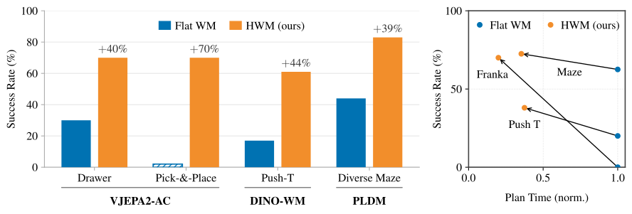
Intuition. To put a cup on a shelf, first plan a useful intermediate grasp and lift, then plan the fine motions that reach it. HWM learns a longer-timescale predictor and compressed macro-actions on top of a shorter-timescale visual world model. Both levels share a state representation, so the high-level model’s predicted next state can become the low-level planner’s goal. At test time, it searches over actions rather than running a separately trained hierarchical policy. The framework improves the studied long-horizon simulated tasks and supports real Franka manipulation from a goal image. Shared latent geometry, finite rollout accuracy and the reachability of proposed subgoals remain limitations; this is distinct from October’s H-JEPA, which learns a separate representation at each level.
1 Introduction
A direct goal-matching optimizer may favor a greedy shortcut even when success requires first moving away from the goal, and long rollouts compound prediction errors. HWM addresses these problems with learned temporal abstraction and top-down subgoal planning. Its high-level action space compresses primitive-action chunks, reducing the search dimension while keeping planning task-agnostic.
2 Hierarchical Planning with Latent World Models
The agent receives current and goal observations and searches under offline-trained latent dynamics. Receding-horizon execution repeatedly observes feedback. The hierarchy changes how this search is organized; it does not provide a reward-trained controller or assume known physical dynamics.
2.1 Learning Multi-Timescale Latent World Models
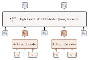
The low-level model predicts short transitions. A learned action encoder summarizes longer primitive-action chunks into macro-actions, and a high-level predictor forecasts their endpoints in the same latent state space. Fewer long-scale rollout steps reduce compounding error, while action compression shrinks the search space. The shared representation enables direct subgoal matching but limits level-specific abstraction.
2.2 Top-Down Hierarchical Planning
The high-level optimizer chooses macro-actions toward the final goal. Its next predicted latent waypoint becomes a target for a short-horizon primitive-action optimizer. Only an initial part is executed before replanning, allowing new observations to correct both levels. Predicted waypoints still have to be physically reachable by the low-level planner.
Equations
3 Empirical Evaluation of Hierarchical Planning Across World Models
The same planning principle is instantiated with V-JEPA2-AC, DINO-WM and PLDM. Real manipulation, longer Push-T episodes and held-out maze layouts test different failure modes; their backbones and data are not identical.
3.1 Franka Arm with Robotiq Gripper
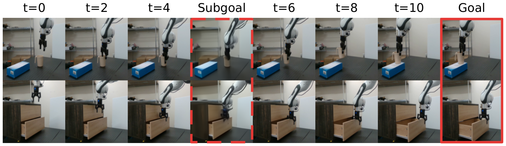
The Franka evaluation includes pick-and-place and drawer tasks with five trials per configuration. A matched flat world-model baseline helps isolate hierarchy; vision-language-action comparators use differing conditioning and sometimes extra camera information. The trial breakdown matters because success rates reflect configuration difficulty as well as stochastic execution.
| Method | P&P Cup | P&P Box | Drawer |
| Octo | 0% | 0% | 43% |
| -FAST-DROID | 52% | 18% | – |
| -DROID | 68% | 36% | – |
| VJEPA2-AC | 0% | 0% | 30% |
| VJEPA2-AC (hierarchy) | 70% | 60% | 70% |
3.2 Push-T
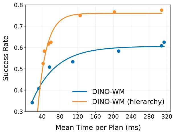
Push-T start–goal pairs extend beyond the shorter horizons of the original DINO-WM setup. Two-level cross-entropy planning is compared with flat planning and offline goal-conditioned policies. Gains are interpreted together with the planning compute budget rather than as a task-independent hierarchy advantage.
| Method | |||
| GCIQL | |||
| HIQL | |||
| HILP | |||
| DINO-WM | |||
| DINO-WM (hier.) | 89% | 78% | 61% |
3.3 Diverse Maze
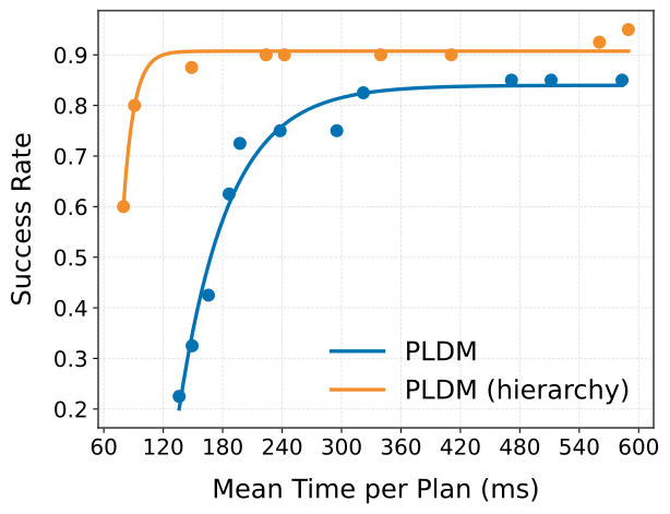
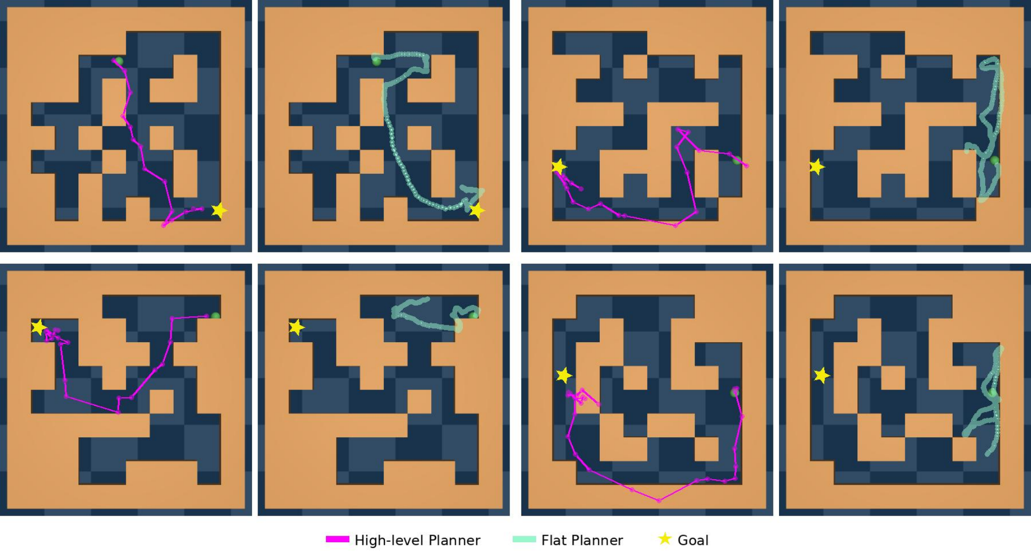
Diverse Maze uses image observations and held-out layouts with increasingly distant goals. Hierarchical path-integral planning improves the reported long-range results over a flat PLDM planner. Generalization is to the described layout distribution, not arbitrary environments or unseen dynamics.
| Method | |||
| GCIQL | 85% | 40% | 33% |
| HIQL | 88% | 73% | 48% |
| HILP | 48% | 20% | 10% |
| PLDM | 100% | ||
| PLDM (hier.) | 100% | 95% | 83% |
3.4 Ablations and Analysis
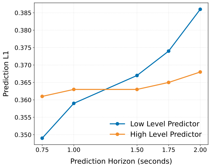
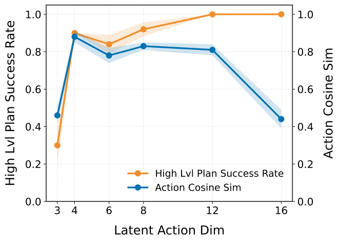
The short-timescale predictor is more accurate nearby, while the long-timescale predictor becomes more accurate at longer horizons in the tested robot data. Macro-action and capacity ablations show that extra parameters alone do not explain the reported gains. Subgoal usefulness depends on both being a plausible future state and being reachable by lower-level search.
| Action | ||
| Concatenated | 52% | 37% |
| Macro-actions | 95% | 83% |
| Action | Cos | |
| Delta pose | ||
| Macro-actions |
4 Related Works
The paper separates predictive world-model planning from hierarchical policies that amortize actions through task-oriented learning, and from controllers using known dynamics. Earlier temporal abstraction ideas remain foundational; the contribution is a modular hierarchy over visual latent models trained through prediction.
| Method | Zero-shot | Representation | Training | Hierarchical Interface |
| HWM (ours) | ✓ | pixels latent | Next-latent pred. | Subgoal matching (latent) |
| CAVIN [20] | ✓ | structured state | Learned dynamics | Subgoal matching (state) |
| LAT [21] | ✓ | structured state | Learned dynamics | Skill-conditioned policy |
| Safe HMPC [22] | structured state | Analytical dynamics | Reference tracking | |
| IQL-TD-MPC [42] | state latent | Offline RL + MPC | Goal-conditioned policy | |
| Director,Puppeteer [14, 19] | pixels latent | Model-based RL | Goal-conditioned policy | |
| THICK [17] | pixels latent | MB-RL + reward | Subgoal matching (latent) |
5 Conclusion
High-level predictions can provide useful intermediate goals without manual decomposition at deployment. The experiments support this mechanism across several backbones, but every tested method still degrades as tasks become harder or longer.
6 Limitations
A shared representation simplifies transferring subgoals but may retain detail unnecessary at higher levels. High-level waypoints are determined by temporal sampling and macro-action design, and may be difficult for low-level planning. Learned subgoal discovery and feedback from low-level feasibility are proposed improvements.
Appendix Contents
Appendix A Training Details
A.1 Low Level World Model
The low-level objective combines teacher-forced next-latent prediction with an autoregressive rollout term. These two losses train local accuracy and behavior under self-generated context, respectively; rollout training does not remove long-horizon model bias.
Equations 1–3
| (1) | ||||
| (2) |
| (3) |
A.2 Franka Arm with Robotiq Gripper
Robot data combines DROID and RoboSet trajectories with visual observations, end-effector proprioception and pose-change actions. Sampling frame rates and action/state conventions are retained because they define the temporal scale of the learned macro-actions.
| World Model | Epochs | Batch Size | context | ||
| VJEPA2-AC (Low-Level) | 200 | 256 | 1.0 | 1.0 | 16 |
| VJEPA2-AC (High-Level) | 120 | 768 | 1.0 | 0.0 | 3 |
A.3 Push-T
Push-T uses the released DINO-WM dataset and frozen DINOv2 features. Actions are chunked across the image stride. The high-level predictor changes temporal abstraction on top of this backbone rather than retraining all visual perception end to end.
| World Model | Epochs | Batch Size | context | ||
| DINO-WM (Low-Level) | 100 | 256 | 1.0 | 0.0 | 4 |
| DINO-WM (High-Level) | 500 | 128 | 1.0 | 0.0 | 5 |
A.4 Diverse Maze
Random maze trajectories span many layouts and velocities; held-out layouts test navigation generalization. The main text’s10-by-10 layout includes the outer boundary, while the appendix describes the 8-by-8 interior grid. Velocity and coverage remain important to interpretable comparisons.
| World Model | Epochs | Batch Size | lr | pred | |||||||
| PLDM (Low-Level) | 3 | 128 | 0.018 | 29.4 | 17.9 | 2.80 | 4.81 | 0.0 | 1.0 | 14 | 2.42 |
| PLDM (High-Level) | 5 | 128 | 0.018 | – | – | – | – | 0.0 | 1.0 | 6 | 1 |
Appendix B Planning Details
CEM and MPPI have different low- and high-level budgets. Primitive actions have physical units, whereas macro-action scale comes from training, so their search distributions require different calibration. Full sampling and replanning settings are preserved for reproducing compute–success tradeoffs.
Equations
| # elites | # iters | # samples | Var EMA | ||||
| Franka | 1 | – | 20 | 15 | 2400 | 0.75 | 6 |
| Push-T () | 5 | 10 | 30 | 30 | 300 | 0 | 5 |
| Push-T () | 5 | 20 | 10 | 30 | 1200 | 0.9 | 10 |
| Push-T () | 5 | 25 | 20 | 20 | 1000 | 0 | 15 |
| High-level planner | Low-level planner | |||||||||||
| # elites | # iters | # samples | Var EMA | # elites | # iters | # samples | Var EMA | |||||
| Franka | 1 | – | 22 | 15 | 3000 | 0.65 | 2 | 12 | 5 | 800 | 0.25 | 2 |
| Push-T() | 5 | 10 | 10 | 20 | 900 | 0 | 2 | 10 | 30 | 300 | 0 | 5 |
| Push-T() | 5 | 20 | 10 | 40 | 1500 | 0.9 | 4 | 10 | 20 | 900 | 0.8 | 5 |
| Push-T() | 5 | 25 | 10 | 20 | 1200 | 0.9 | 5 | 10 | 20 | 1200 | 0.8 | 5 |
| noise | # samples | |||||
| Maze () | 4 | 500 | 5 | 125 | 0.0025 | 150 |
| Maze () | 4 | 500 | 5 | 250 | 0.0025 | 200 |
| Maze () | 4 | 500 | 5 | 250 | 0.0025 | 250 |
| High-level planner | Low-level planner | |||||||||
| noise | # samples | noise | # samples | |||||||
| Maze () | 4 | 265 | 10 | 2000 | 0.0025 | 25 | 5 | 500 | 0.0025 | 10 |
| Maze () | 4 | 365 | 10 | 2000 | 0.0025 | 35 | 5 | 500 | 0.0025 | 10 |
| Maze () | 4 | 485 | 10 | 4000 | 0.0025 | 47 | 5 | 1000 | 0.0025 | 10 |
Appendix C Computational Analysis Details
C.1 Push-T
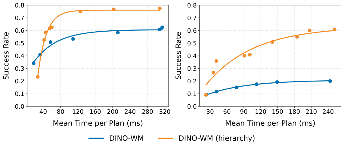
Compute frontiers are obtained by sweeping candidate counts, iterations and distribution smoothing at several Push-T horizons. This compares optimized configurations across budgets instead of one arbitrarily chosen runtime setting.
C.2 Diverse Maze
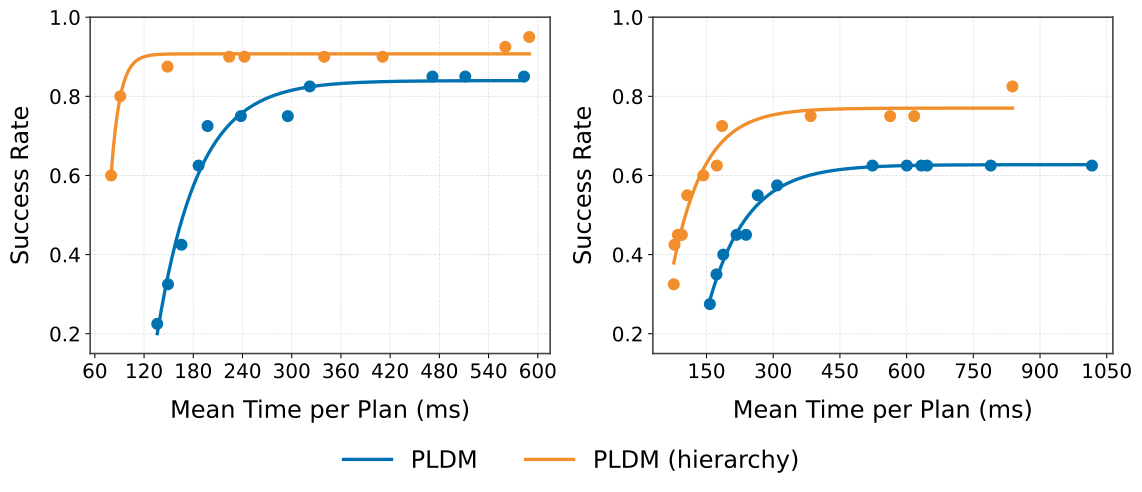
Maze frontiers vary flat horizons and both levels’ sampling budgets. Measured wall-clock comparisons depend on the implementation, model shapes and hardware; they are not operation-count guarantees for every planner.
Appendix D Additional Ablations and Analysis
D.1 Model Size vs. Hierarchy
Larger flat models fail to reproduce the hierarchical gains in the capacity controls. This supports the importance of planning structure in the studied settings, without proving that no differently trained flat model could match it.
D.2 Strides for Fixed Interval Waypoints
A moderate temporal stride helps, but excessive abstraction eventually hurts predictive fidelity and success. The optimal stride therefore balances fewer high-level steps with enough information for reliable subgoals.
| High-level stride | 6 | 8 | 10 | 12 | 14 |
| Success Rate () | 50% | 55% | 77% | 78% | 75% |
D.3 Emergence of semantic subgoals
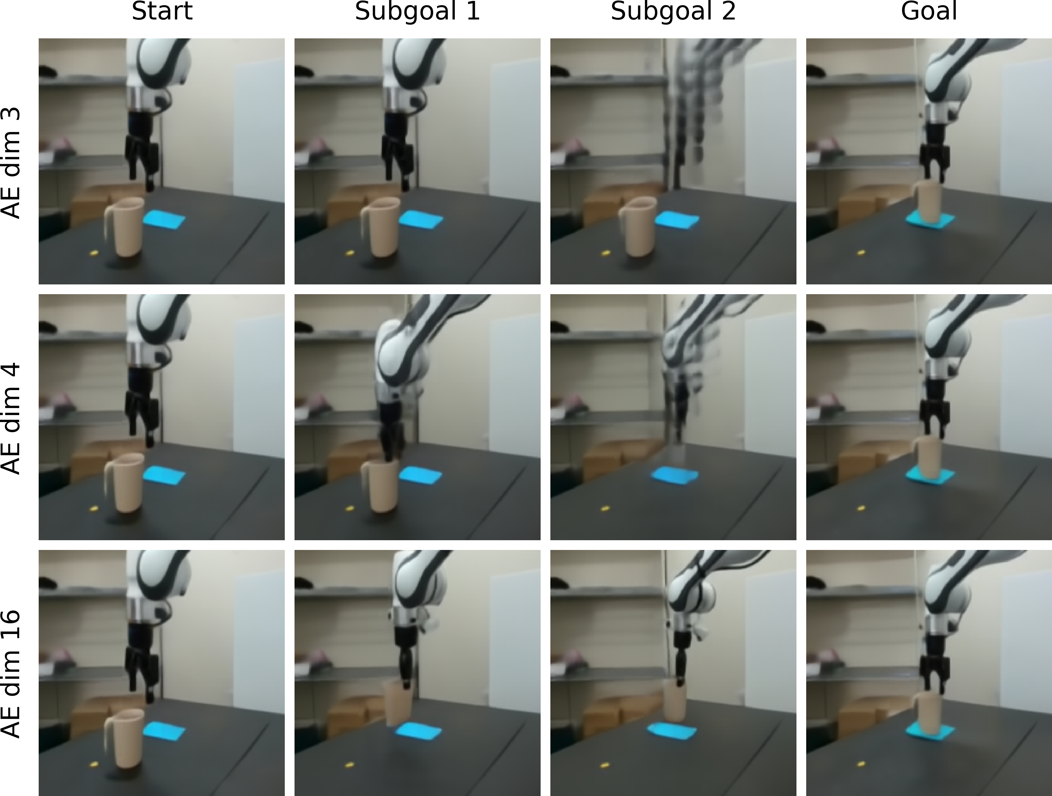
A macro-action bottleneck must be expressive enough for useful transitions but restrictive enough to avoid complicated, hard-to-reach subgoals. The reported Franka choice reflects this tradeoff. A visually meaningful high-level prediction does not automatically imply low-level executability.
Appendix E Manual Subgoals: Isolating Planning from Representation
Manually supplying intermediate grasp images lets the flat planner solve tasks it fails end to end. This control separates planning-objective difficulty from a complete absence of useful dynamics. Such supervised subgoals are a diagnostic, not part of the autonomous HWM deployment protocol.
Appendix F Visualizing World Model Predictions
Separate decoders visualize high-level latent predictions and execution trajectories. Decoder training is not part of the reward-free world-model objective, and a plausible decoded image cannot alone certify a feasible robot motion.
Appendix G Robot Task Definitions
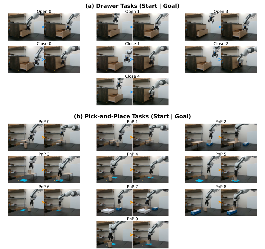
The retained initial and goal images specify pick-and-place and drawer configurations. Box tasks use the same arrangements as cup tasks with a different manipulated object.
Appendix H Per-Configuration Trial Breakdown for Franka
Per-configuration counts and exact confidence intervals accompany aggregate success. Outcomes are largely repeatable within a configuration, so variability across task arrangements is an important source of the aggregate rates.
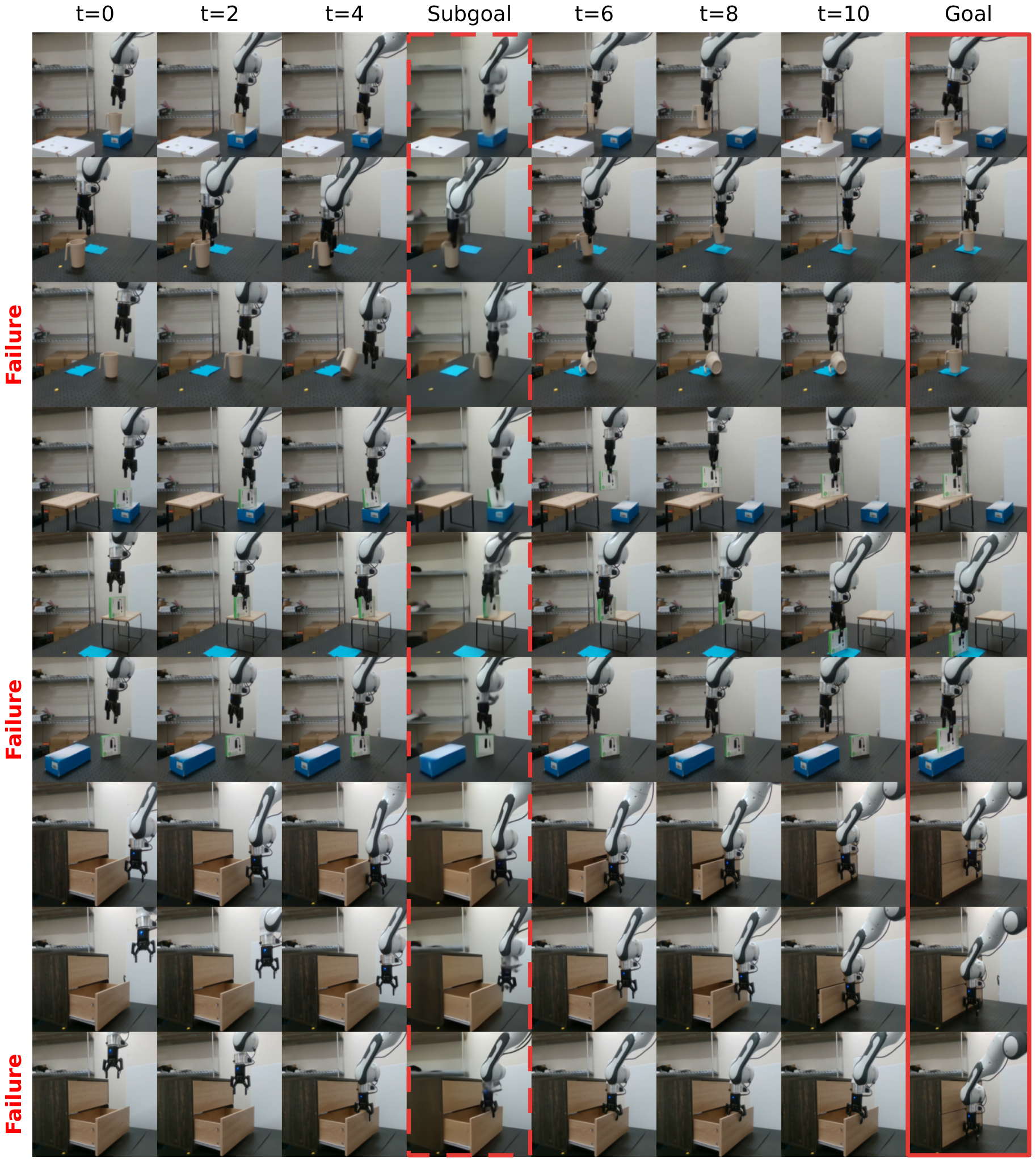
Appendix I Additional Execution Rollouts for Franka
Additional Franka execution sequences retain inferred subgoals and actual motion, allowing comparison between planned intermediate images and execution.
Appendix J Execution Rollout Examples for Push-T
Additional Push-T rollouts retain high-level subgoals and the corresponding lower-level action execution. These selected examples supplement the aggregate evaluation.

Appendix K Offline Planning Evaluation for Franka
An offline proxy compares planned action aggregates with expert directions for the evaluated manipulation configurations. It permits faster iteration but uses manually specified subgoal structure and cannot substitute for all closed-loop robot trials.
Appendix L Baselines
L.1 Vision-Language-Action Models
Camera, conditioning and checkpoint choices for the vision-language-action models are documented. Some policy baselines consume wrist images or language goals unavailable to the world-model planner, so the comparison is informative but not a perfectly matched ablation.
L.2 Goal-Conditioned & Zero-Shot RL Methods
Goal-conditioned IQL, hierarchical IQL and HILP use learned policies or value geometry rather than online predictive search. Their official implementations and per-difficulty tuning are retained to separate baseline construction from the hierarchy claim.
| GCIQL | HIQL | HILP | |||||||
| lr | expectile | rand goal | lr | expectile | rand goal | alpha | lr | expectile | |
| Push-T() | 0.6 | 0.0 | 0.9 | 0.0 | 3.0 | 0.6 | |||
| Push-T() | 0.6 | 0.3 | 0.9 | 0.3 | 1.0 | 0.6 | |||
| Push-T() | 0.9 | 0.6 | 0.9 | 0.3 | 1.0 | 0.6 | |||
| Maze() | 0.8 | 0.0 | 0.6 | 0.3 | 1.0 | 0.9 | |||
| Maze() | 0.6 | 0.3 | 0.8 | 0.6 | 3.0 | 0.9 | |||
| Maze() | 0.6 | 0.0 | 0.8 | 0.6 | 3.0 | 0.9 | |||