At a glance
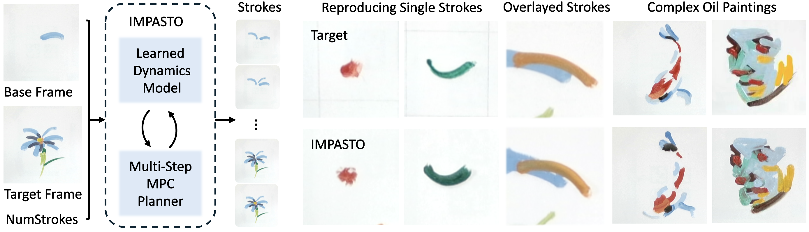
IMPASTO combines a robot-trained image dynamics model, stroke planning and force-sensitive brush control to reproduce oil paintings from intermediate target images. The model predicts the next canvas patch from the current patch and a candidate stroke. Planning searches for strokes whose predicted results match the target, then uses new camera observations to correct execution errors. Experiments cover 60 strokes from five artists, 50 robot-produced overlaid strokes, two short paintings and longer qualitative demonstrations.
I Introduction
Oil painting couples deformable bristles, wet pigment, contact force and stroke order. IMPASTO learns these effects from robot self-play rather than a faithful physics simulator or human action trajectories. It still receives human-produced target images, sometimes step by step; “no demonstrations” means no demonstrated robot controls, not absence of visual supervision.
The system estimates a discrete pigment/opacity choice separately, predicts grayscale canvas changes, searches geometric stroke parameters and executes them on a Franka arm. This edition covers all 14 pages of v1, dated 31 March 2026, including nine main figures, seven appendix figures, two tables, Algorithm 1, all 20 numbered equations and 53 references. Figure numbers follow the PDF because the HTML reset them incorrectly.
II Related Work
II-A Modern Robot Painting
Earlier painting systems range from programmed AARON strokes to visual-feedback e-David and differentiable planning in FRIDA. Learning approaches include reinforcement, imitation and generated stroke models. IMPASTO focuses on reproducing existing wet-paint strokes with a state-conditioned forward model. Its FRIDA-CNN comparator adapts one FRIDA component to this task; it is not an evaluation of the entire original FRIDA workflow.
II-B Planning with Learned Neural Dynamics Models
Visual foresight and related learned dynamics approaches predict consequences in images, latent states or structured geometry. Pixel prediction is natural here because the objective is canvas appearance. Sampling methods such as MPPI avoid requiring smooth action gradients but can be expensive; gradient optimization can encounter local minima. IMPASTO combines image-derived initial guesses with adaptive stochastic refinement.
III Method
We describe the parameterization of brushstrokes, color prediction, the hardware system setup for oil painting, the architecture design and training of the dynamics model, the multi-step planning algorithm, and baseline methods for comparison.
III-A Brushstroke Model
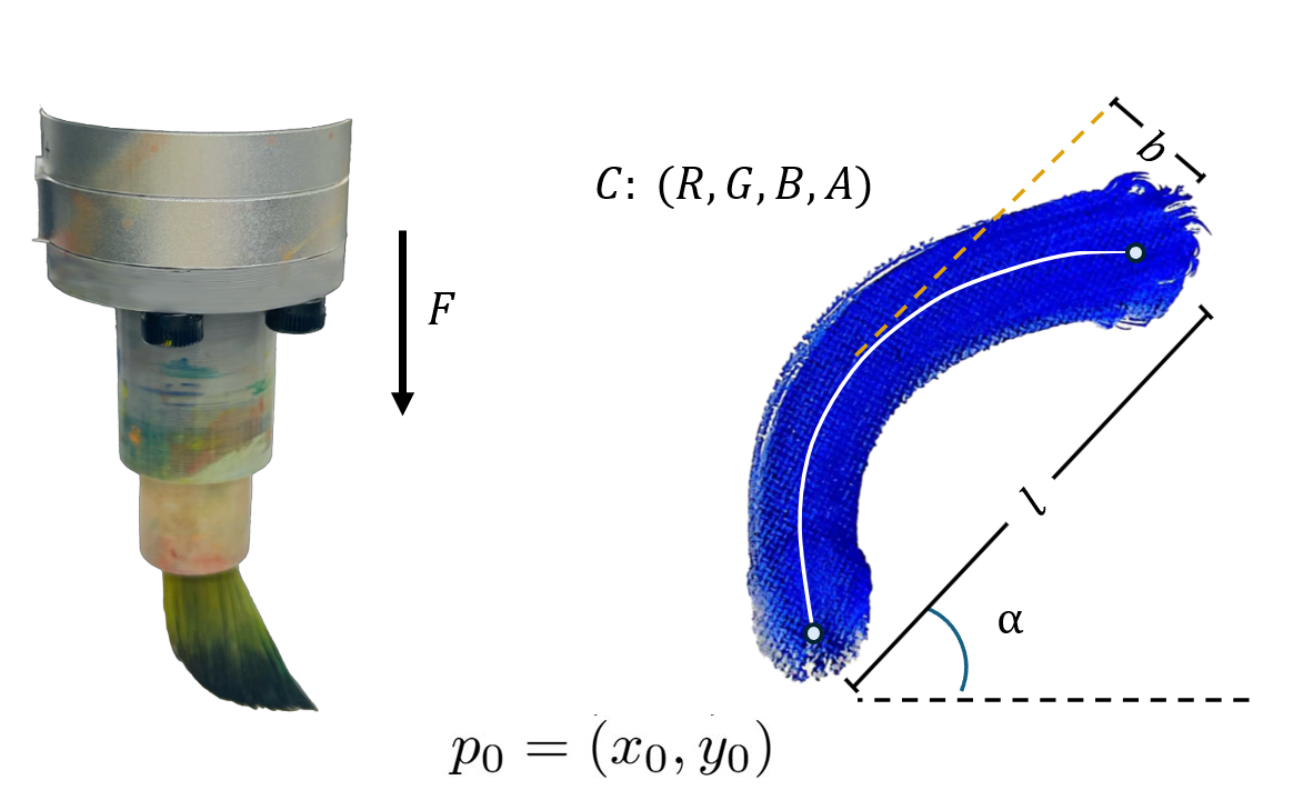
A stroke has six geometric/control coordinates: starting x/y, length, bend, in-plane heading and normal force. A quadratic Bézier curve supplies the centerline; color and transparency are estimated separately. Bounds restrict actions to the calibrated task range. Force replaces the penetration-depth parameter used by related Spline-FRIDA models.
This family represents smooth curved strokes, not arbitrary brush motion. Abrupt direction changes, serif-like endings, changing brush orientation and richer within-stroke force profiles lie outside the stated parameterization. The evaluation controls brush and pigment condition to reduce stochasticity rather than modeling every hidden paint/brush state.
Equation 1
| (1) |
III-B Color Prediction
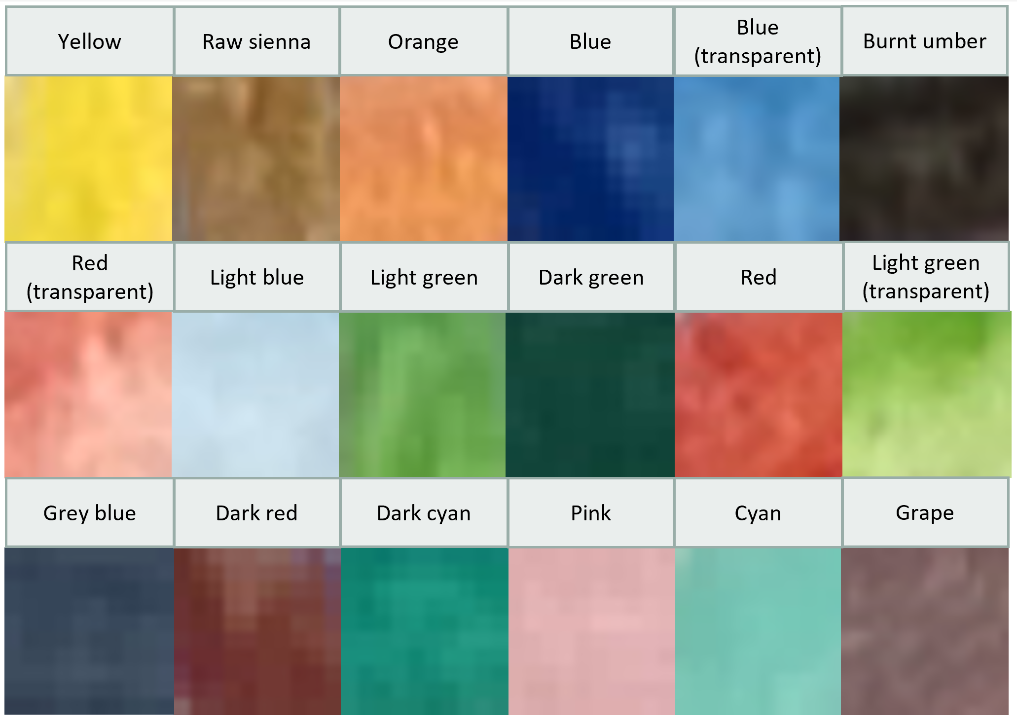
The color module summarizes target pixels within a stroke mask and selects a nearby measured pigment prototype using a covariance-scaled Mahalanobis distance in linear RGB. A ratio comparing observed color change with palette-to-base contrast classifies transparency. This is selection from premixed colors and measured conditions, not unrestricted paint mixing or a learned full-color fluid model.
III-C The Hardware System and Robot Control
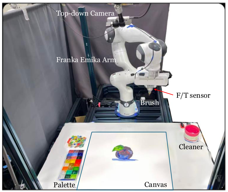
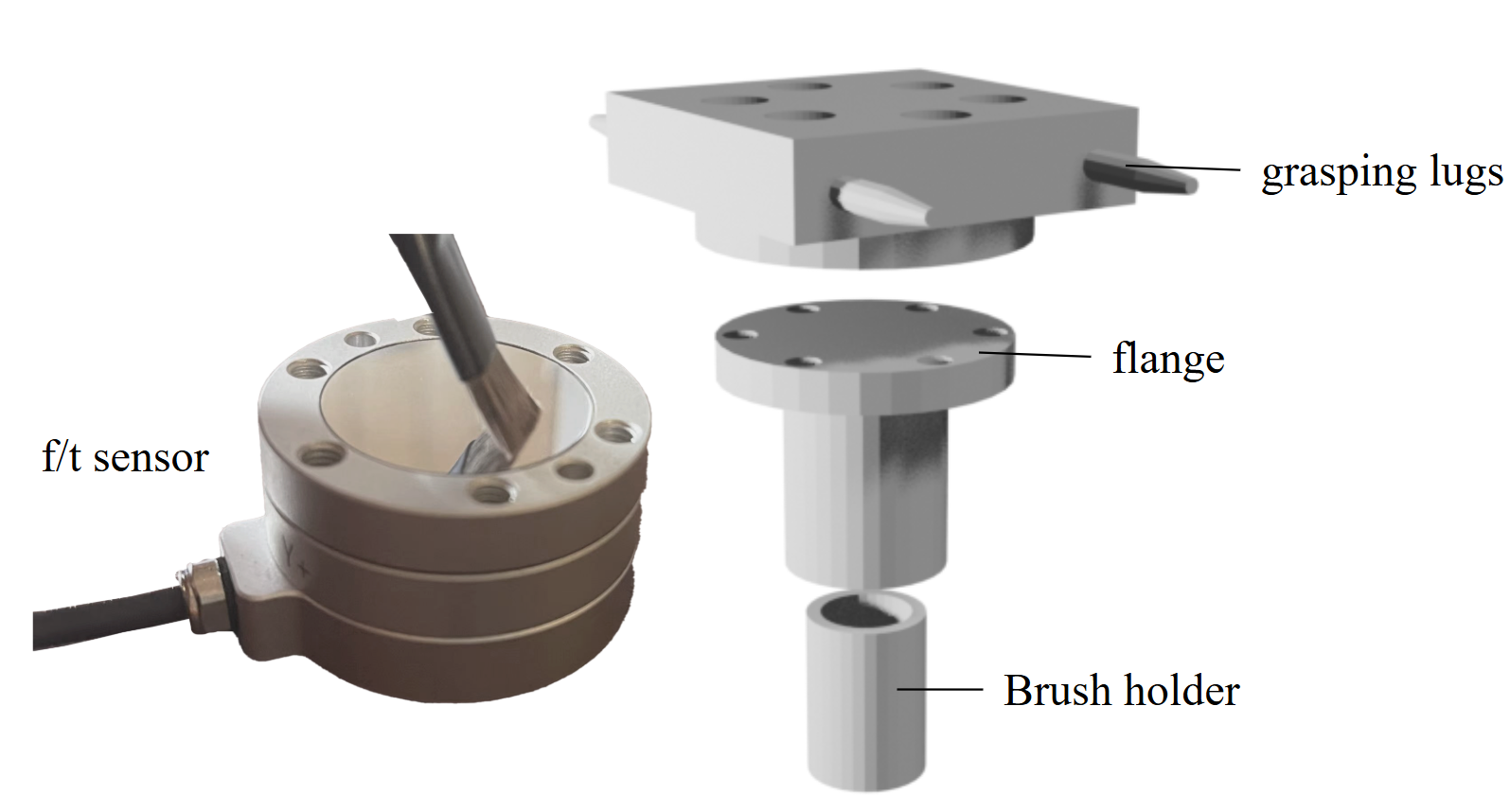
A seven-DoF Franka Panda carries a six-axis force/torque sensor and a size-8 round synthetic brush trimmed to 5 cm, held perpendicular to an 18×21-inch canvas. The reported force range is 0.1–4 N. A top-down RealSense D435 image is undistorted, homography-warped and cropped. Palette trays and a motorized water spinner support dipping and cleaning.
At contact onset, an exponentially filtered force error accumulates a feedforward command that enters joint torque through a Jacobian transpose. After reaching the target force, the robot holds the same vertical position under impedance control for the rest of the stroke. Thus the described controller does not continuously regulate the specified normal force throughout every stroke; its adequacy relies on local canvas flatness and stable contact. Gains, sampling rate and force-tracking error statistics are not supplied.
Equations 2–4
| (2) |
| (3) |
| (4) |
III-D The Pixel Dynamics Model and Training
Pixel dynamics model
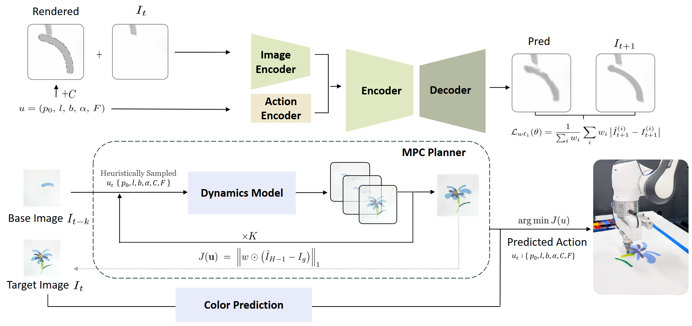
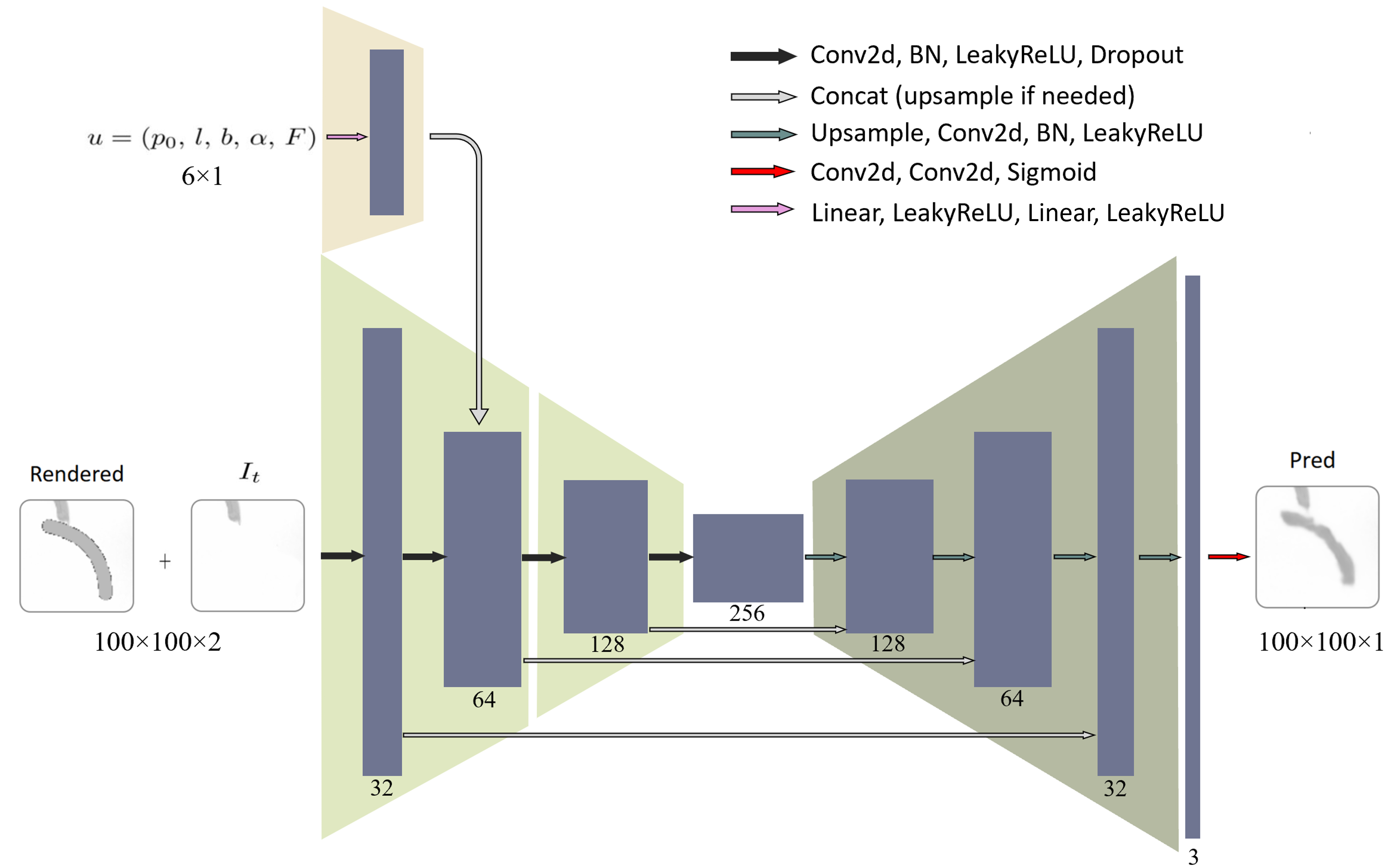
A U-Net image encoder receives the current canvas patch concatenated with a simple rendering of the proposed stroke. A separate encoder processes the six action coordinates, and the decoder fuses both paths to predict the full next patch. The rendered footprint makes position, orientation and width explicit in image space, while the learned component models departures from that simple rendering.
The Bézier midpoint control is offset by the bend along the normal direction; a calibrated force-to-width map sets the footprint. Network patches are 100×100 grayscale images. Color selection therefore operates outside the learned image dynamics, and RGB artwork appearance should not be mistaken for full-color neural state prediction.
Equations 5–7
| (5) |
| (6) | ||||
| (7) |
Dataset and training
Self-play samples stroke location, length, bend, heading and force while cycling fixed colors. Before/action/after tuples supervise a weighted absolute-error loss, normalized by total weight and emphasizing a dilated mask of changed pixels. Slight cropping, rotations and flips augment training; Adam updates the model. The source also states that color-prediction runs use ground-truth color labels, without a separate reported classification-accuracy evaluation.
A single image does not explicitly encode brush loading, residual pigment, wetness or drying history. Controlled conditions make the experiments interpretable, but they limit claims about robustness to arbitrary hidden material state.
Equation 8
| (8) |
III-E Multi-Step Stroke Planning
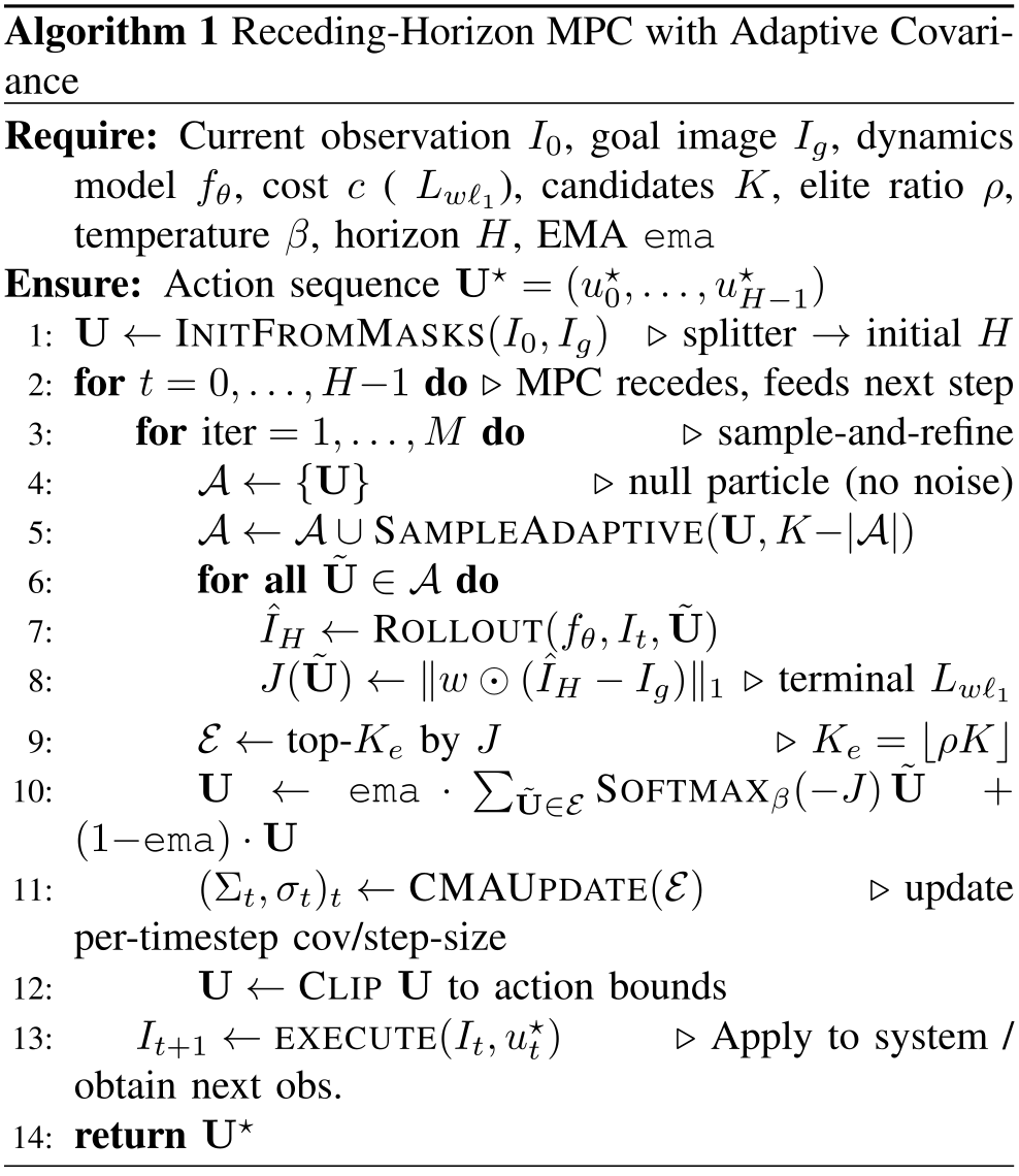
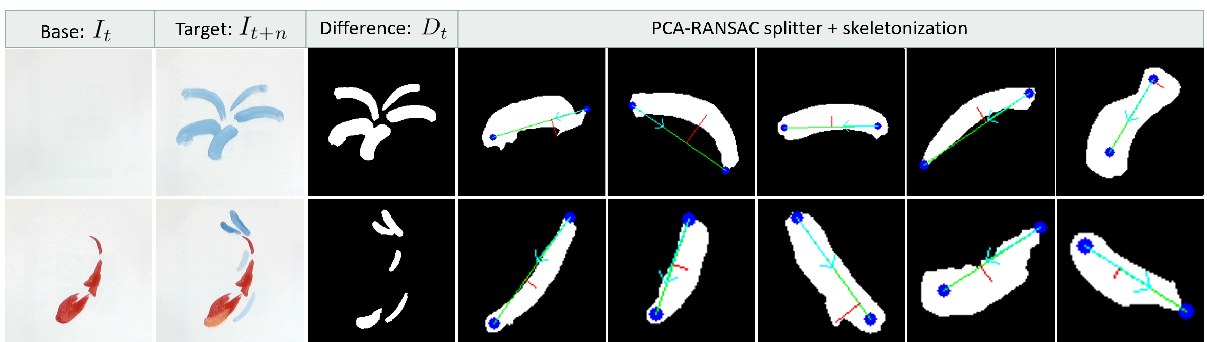
For multi-stroke planning, the prose specifies horizon five and execution of the first two strokes before observing and replanning. A PCA–RANSAC splitter proposes stroke masks; adaptive Gaussian sampling, elite softmax weighting and covariance/step-size updates refine the sequence. Candidates are clipped to action bounds and scored by weighted terminal image error.
The source descriptions differ in detail: Equation 9 uses predicted image ÎH−1, whereas Algorithm 1 scores ÎH; the algorithm executes one indexed action inside its loop rather than explicitly showing the prose’s two-action execution block. Original equations and pseudocode are retained. These indexing/execution ambiguities should be resolved before reproducing the planner; the paper does not establish a general stability or error bound for its closed-loop procedure.
Equation 9
| (9) | |||
Original selectable algorithm
III-F Baseline Methods
IMPASTO-LR fits force to a softplus-transformed affine thickness parameter and stamps a trajectory, then blends a constant-color stroke. Despite the name, the displayed thickness function is not purely linear. Heuristics-only skeletonizes the target difference, derives endpoints/heading/bend and uses fixed force 0.5. FRIDA-CNN predicts a canonical stroke mask from length, bend and force, then transforms and composites it.
These comparators do not condition stroke formation on the existing canvas. They still use the base image when compositing the predicted increment, while U-Net predicts the full next image. That difference may favor preserved background pixels for baselines and contextual overpainting for U-Net; it is not an otherwise identical architecture ablation. The original statement that baselines lack base-state access concerns prediction conditioning, not final compositing.
Equation 10
| (10) |
IV Experiments and Results
Our experiments are designed to address three key questions: . How much data is needed to train a dynamics model in our case? . Can IMPASTO reproduce expert human artists’ strokes with low error and high visual similarity? . Can IMPASTO enable closed-loop, multi-step planning to approximate a given oil painting?
𝒬 𝟏 . Can IMPASTO ’s pixel dynamics model be trained to predict the stroke effects with high fidelity?
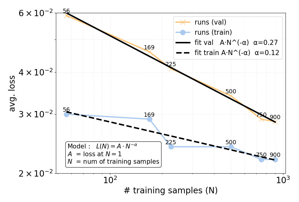
Prediction error decreases with more self-play examples. At 900 training samples the reported unweighted absolute image error is 0.0285; validation uses a fixed 10% of the total collected dataset. Figure 5 shows fitted power-law trends, not a guarantee about larger datasets or other brushes. This unweighted dynamics error is distinct from the weighted planning/execution losses in the later tables. Repeated-training uncertainty and detailed split dependence are not reported.
𝒬 𝟐 . Can IMPASTO reproduce human individual strokes with lower error and higher visual similarity than baseline methods?
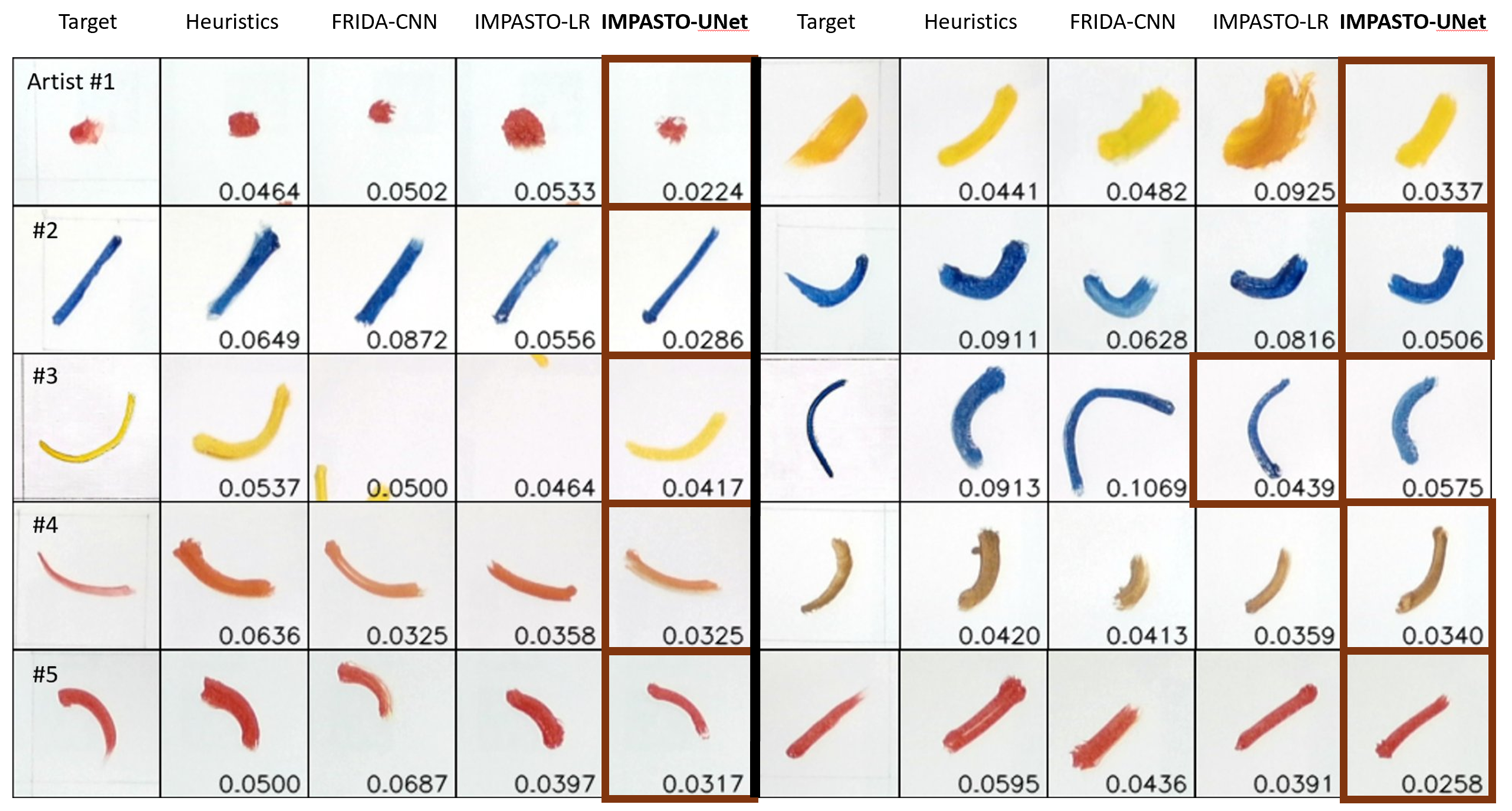
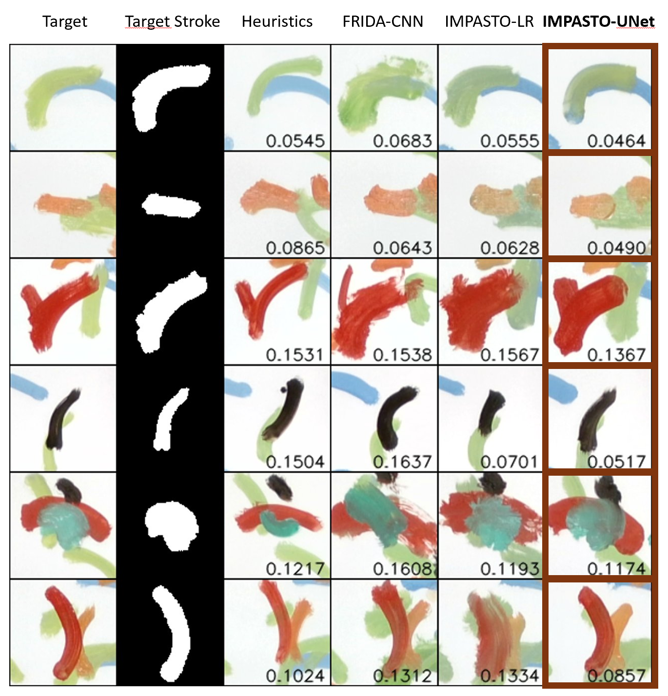
The held-out single-stroke set contains 12 strokes from each of five expert artists, 60 total. A separate 50-stroke overlaid set is produced by the robot, not human experts. One-step planning is evaluated first through predicted images and then through physical execution photographs. Brush and pigment conditions are matched as closely as possible. Weighted pixel error and LPIPS perceptual distance measure different aspects; LPIPS is not a human-rater study.
Across artists, U-Net’s mean planning/execution/LPIPS losses are 0.02224/0.04934/0.18078. Relative to FRIDA-CNN these decrease by 16.45%, 19.48% and 35.36%; relative to LR by 5.28%, 5.33% and 18.21%. Execution pixel error and LPIPS improve over the heuristic by 21.21% and 15.68%. These are relative reductions of averaged losses, not success-rate gains.
U-Net has the lowest LPIPS for every artist, but LR has lower planning pixel error for Artist 3 and lower execution pixel error for Artists 3, 4 and 5. On the robot overlaid set, U-Net gives 0.0258 planning, 0.0907 execution and 0.2209 LPIPS, best among the listed methods. No repeated-execution uncertainty, significance tests or blinded aesthetic assessments are provided; controlled conditions and examples support a scoped reproduction result.
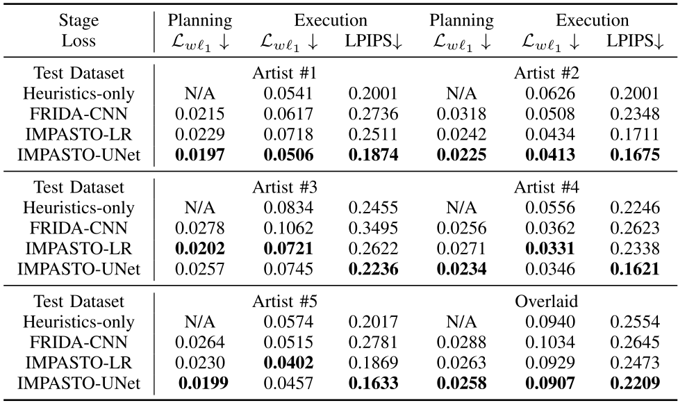
Original selectable table
| Stage | Planning | Execution | Planning | Execution | ||
|---|---|---|---|---|---|---|
| Loss | LPIPS | LPIPS | ||||
| Test Dataset | Artist #1 | Artist #2 | ||||
| Heuristics-only | N/A | 0.0541 | 0.2001 | N/A | 0.0626 | 0.2001 |
| FRIDA-CNN | 0.0215 | 0.0617 | 0.2736 | 0.0318 | 0.0508 | 0.2348 |
| IMPASTO-LR | 0.0229 | 0.0718 | 0.2511 | 0.0242 | 0.0434 | 0.1711 |
| IMPASTO-UNet | 0.0197 | 0.0506 | 0.1874 | 0.0225 | 0.0413 | 0.1675 |
| Test Dataset | Artist #3 | Artist #4 | ||||
| Heuristics-only | N/A | 0.0834 | 0.2455 | N/A | 0.0556 | 0.2246 |
| FRIDA-CNN | 0.0278 | 0.1062 | 0.3495 | 0.0256 | 0.0362 | 0.2623 |
| IMPASTO-LR | 0.0202 | 0.0721 | 0.2622 | 0.0271 | 0.0331 | 0.2338 |
| IMPASTO-UNet | 0.0257 | 0.0745 | 0.2236 | 0.0234 | 0.0346 | 0.1621 |
| Test Dataset | Artist #5 | Overlaid | ||||
| Heuristics-only | N/A | 0.0574 | 0.2017 | N/A | 0.0940 | 0.2554 |
| FRIDA-CNN | 0.0264 | 0.0515 | 0.2781 | 0.0288 | 0.1034 | 0.2645 |
| IMPASTO-LR | 0.0230 | 0.0402 | 0.1869 | 0.0263 | 0.0929 | 0.2473 |
| IMPASTO-UNet | 0.0199 | 0.0457 | 0.1633 | 0.0258 | 0.0907 | 0.2209 |
𝒬 𝟑 . Can IMPASTO enable closed-loop, multi-step planning to approximate complex oil paintings?
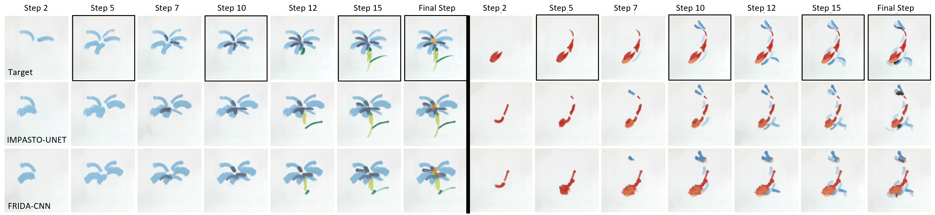
The controlled multi-step comparison uses Flower and Fish, containing 17 and 18 artist strokes. Targets include images after steps 5, 10, 15 and the final stroke; the planner therefore receives intermediate progress images rather than only a final artwork. Both U-Net and FRIDA-CNN use horizon five.
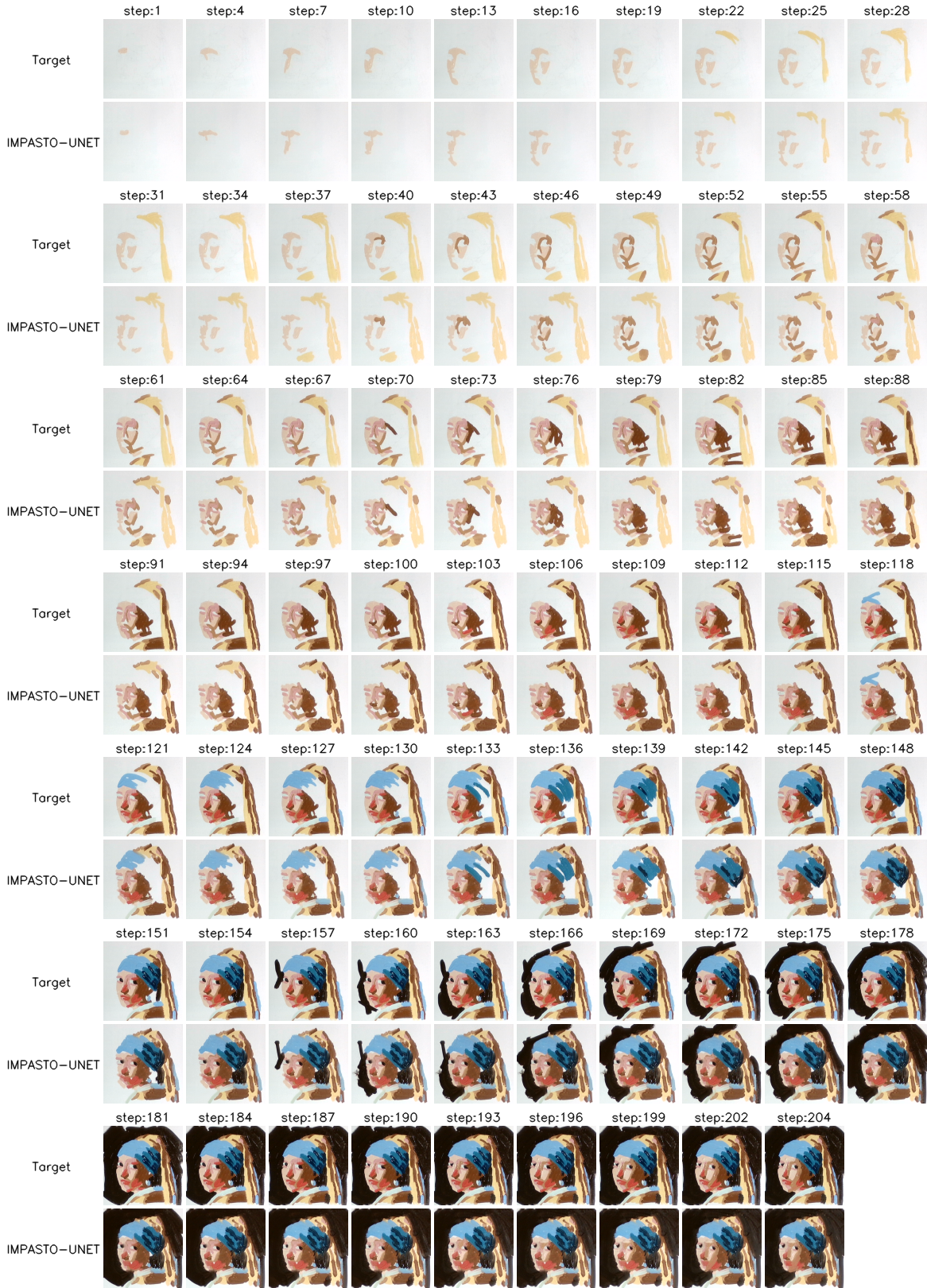
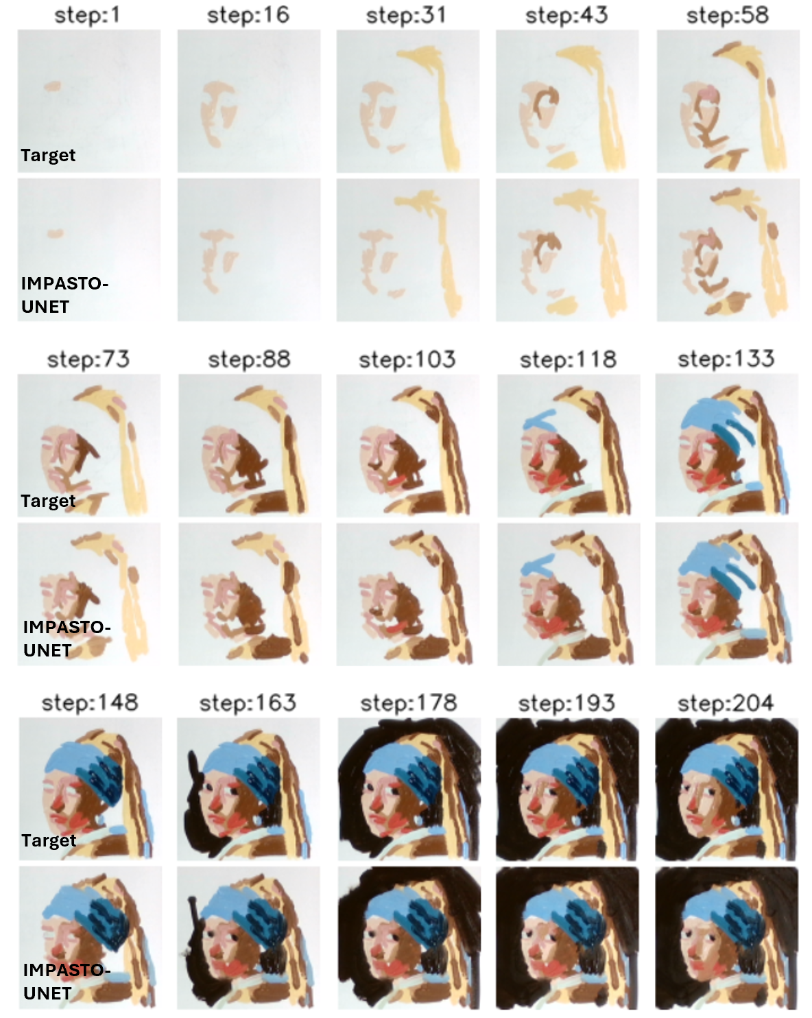
For Flower, U-Net’s planning/execution/LPIPS losses are 0.0427/0.0464/0.1293 versus 0.0597/0.0501/0.1619. For Fish they are 0.0421/0.0452/0.1117 versus 0.0519/0.0523/0.1204. Averaged relative reductions are 24.01%, 10.55% and 14.63%. These are two artwork comparisons without reported replication uncertainty. The 204-stroke example demonstrates a longer reproduction sequence; Appendix D identifies its mode as step-by-step artist following with CMA-ES, not a 204-action joint optimization from a final image.

V Conclusions
The main result is a physical system that learns local stroke consequences from self-play and uses them to improve constrained painting reproduction. Its strongest controlled evidence is the stroke-level comparison and two short multi-stroke paintings. Generalization to new brushes, pigments, surfaces, drying conditions and arbitrary final-image decomposition remains untested. Runtime, planning sample counts and calibration/control constants are incompletely reported, and the longer artworks are qualitative demonstrations.
ACKNOWLEDGMENT
This work is in part supported by the Stanford Institute for Human-Centered AI (HAI), the Schmidt Futures Senior Fellows grant, ONR MURI N00014-21-1-2801, ONR MURI N00014-22-1-2740, ONR MURI N00014-24-1-2748, and NSF RI #2211258.
Appendix A. Robotic Hardware System
The printed mount connects gripper lugs, the force sensor flange and brush holder. Grounding reduces acquisition noise; a short stationary window estimates sensor bias before each primitive, followed by exponential smoothing. This filter’s coefficient weights the new sample, while the main force-error filter’s λ weights the previous estimate, so the two displayed conventions should not be interchanged.
RGB capture is 1920×1080. Training uses distributed data parallelism on NVIDIA RTX A5000, RTX 3090 and A40 GPUs; deployment uses RTX 4090 hardware. Device names alone do not establish planning latency or real-time throughput.
Equation 11
| (11) |
Appendix B. Learning the Dynamics Models
The detailed architecture uses U-Net skip connections, an action branch and a single-channel output. Adam trains for 1,000 epochs with batch size 120, learning rate 5×10⁻⁴ and weight decay 10⁻³; the rate is multiplied by 0.75 every 100 epochs.
A simple rasterizer stamps filled circles along a straight or quadratic centerline. Radius follows rmin+kFγ, with positive γ. It renders identical RGB channels for grayscale-loader compatibility and fully opaque alpha, then resizes to 100×100. This rendering prior differs from the separately estimated physical color/transparency choice; learned corrections, rather than the prior alone, produce the final state prediction.
Equation 12
| (12) |
Baseline Implementation Details
Topology-preserving thinning produces a one-pixel skeleton. Endpoint degree in an eight-neighbor graph determines candidates; endpoint displacement gives length and heading, and the largest signed normal deviation gives bend. Branches or poorly defined endpoints can challenge this restricted representation; the paper does not quantify these failures.
FRIDA-CNN maps three canonical parameters through batch normalization, an MLP and convolution into a 100×100 occupancy mask. Position/heading transform the mask; opacity is clipped and used in a convex blend of base image and scalar stroke color. All baselines share this state-independent incremental-stroke interpretation.
Equation 13
| (13) |
Color Prediction Module
The tray has 24 physical slots, with only a task-specific subset used. A measured 25×25 patch database includes multiple color/transparency conditions. For single strokes, a thresholded base–target difference and distance-transform weights select pixels; for multi-step planning, the rendered stroke foreground is intersected with a disk around its geometric center.
A weighted mean in linear RGB is classified by the nearest prototype under that label’s estimated covariance. Transparency is decided from median observed change divided by median palette-to-base contrast plus a safety constant. Threshold, disk radius, covariance regularization and quantitative classifier errors are not specified. The ratio is a heuristic for these measured materials, not a physical model of arbitrary pigment mixing.
Equations 14–15
| (14) |
| (15) |
Equations 16–17
| (16) |
| (17) |
Appendix C. Planning
PCA-RANSAC multi-way splitter
The splitter clusters changed pixels using normalized spatial coordinates, computes a local PCA frame, then uses RANSAC to fit a line or quadratic. Candidate inliers are scored for uncovered area with penalties for curvature and overlap. Centerline seeding and constrained region growth thicken the selected nonoverlapping masks into stroke initializations.
The appendix uses K for the number of candidate stroke masks and later for the number of sampled action sequences, while the main planner asks for H stroke initializations. These roles should be distinguished in an implementation. Mask decomposition is a heuristic, not evidence of uniquely recovering an artist’s original stroke sequence.
Equations 18–19
| (18) |
| (19) |
Stochastic Sampling with CMA-Style Adaptive Covariance
Each iteration retains the nominal sequence as a noise-free candidate and samples the others with per-time-step Gaussian perturbations σtAtzt, where AtAt⊤=Σt. After clipping and rollout, the lowest-cost elite set receives temperature-softmax weights; its mean updates the nominal sequence by exponential averaging.
CMA-style evolution paths adapt step sizes and covariance matrices, including a rank-μ contribution. The paper names these updates but does not supply complete update equations, candidate/elite counts, temperature, iteration count or timing. It is an MPPI-style weighted search with CMA-style adaptation; the longer demonstrations are separately described as using CMA-ES.
Equation 20
| (20) |
Appendix D. Additional Results
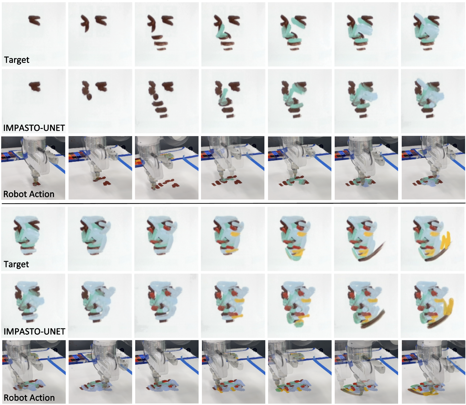
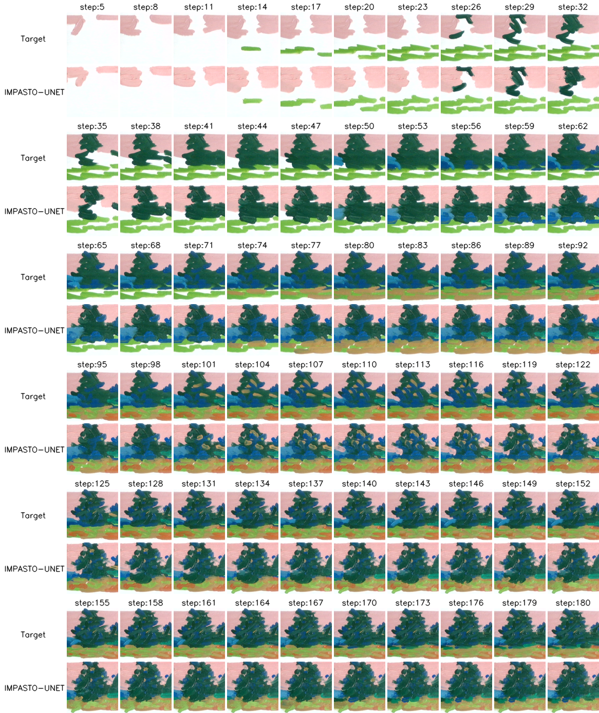
All appendix montages are retained: a 40-stroke portrait with robot-action photographs, a 180-stroke landscape and a 204-stroke portrait. They compare selected human and robot intermediate images, with the latter portrait also appearing in the main text. The stated procedure follows the human artist step by step using CMA-ES. These examples show sustained physical execution under supplied intermediate goals, without a quantitative long-artwork baseline or proof of autonomous stroke-order discovery.