Overview
This edition covers all fifteen pages of arXiv v1, dated 28 March 2026, including the supplementary camera/depth losses, ablations, additional benchmarks and qualitative comparisons. Weibang Wang, Kenan Li and Zhuoguang Chen contributed equally; Yijun Yuan and Hang Zhao jointly advised the work.
At a glance
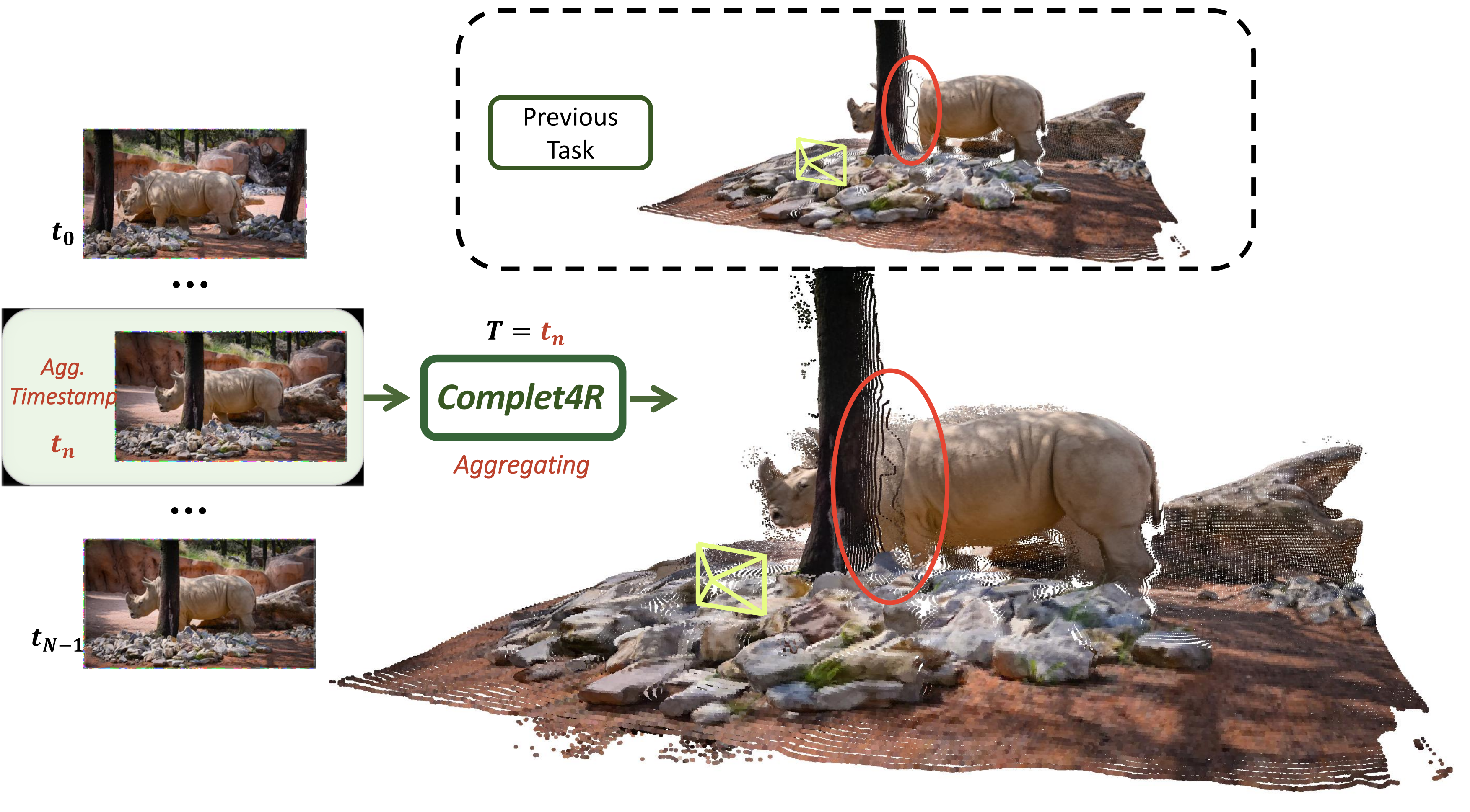
Complet4R takes a monocular video and a target timestamp, then predicts where points observed throughout the video lie at that time. Combining these predictions recovers surfaces occluded in the target image but visible elsewhere in the sequence.
A transformer initialized from VGGT uses target-specific tokens, global attention and a focal-weighted point loss. It improves a new synthetic completion benchmark and scale-aligned 3D tracking. “Complete” refers to geometry observed somewhere in the input, not arbitrary never-observed surfaces or guaranteed watertight objects.
1 Introduction
Static reconstruction combines views under a rigid-scene assumption. Dynamic methods must additionally estimate where moving surfaces go; reconstructing only each frame’s visible points leaves holes when surfaces become occluded.
Complet4R aggregates all observed geometry into a chosen time and repeats this operation for other times to form trajectories. This makes completion and tracking two uses of the same prediction, rather than stitching only pairwise correspondences. Its evidence concerns geometric accuracy and track consistency; the paper’s broader language about physical causality is not an independently tested causal model.
2 Related Work
The related work separates camera/scene reconstruction, dynamic 4D reconstruction and point tracking. These families differ in their inputs, outputs and treatment of occlusion.
2.1 Camera Estimation and Scene Reconstruction
SfM/SLAM estimate rigid geometry and camera motion through matching and optimization. Feed-forward DUSt3R, MASt3R and VGGT predict geometry more directly; MonST3R, MegaSaM and CUT3R extend this direction to dynamic scenes.
Many such methods still output the visible geometry of each frame. Temporal completion additionally needs to place surfaces seen at other times into the current dynamic configuration.
2.2 4D Reconstruction
RGB-D fusion, nonrigid reconstruction, neural radiance fields and Gaussian splatting model moving scenes with different observation and optimization assumptions. Several recent generative methods emphasize photorealistic novel views.
Complet4R instead predicts geometry directly from a monocular sequence. St4RTrack and related 4D point-map methods establish correspondence, but their original formulations do not directly aggregate all observed points into each target timestamp.
2.3 3D Point Tracking
Long-range 2D trackers exploit temporal and spatial context but do not directly supply world-coordinate motion. SpatialTracker methods lift tracking into 3D; SpatialTrackerV2 also estimates camera motion.
Sparse or pairwise tracking can require subsequent alignment and accumulation for dense completion. Complet4R shares the global temporal reasoning needed by both tasks, although its finite benchmark results do not guarantee drift-free trajectories.
3 Geometric Complete 4D Reconstruction
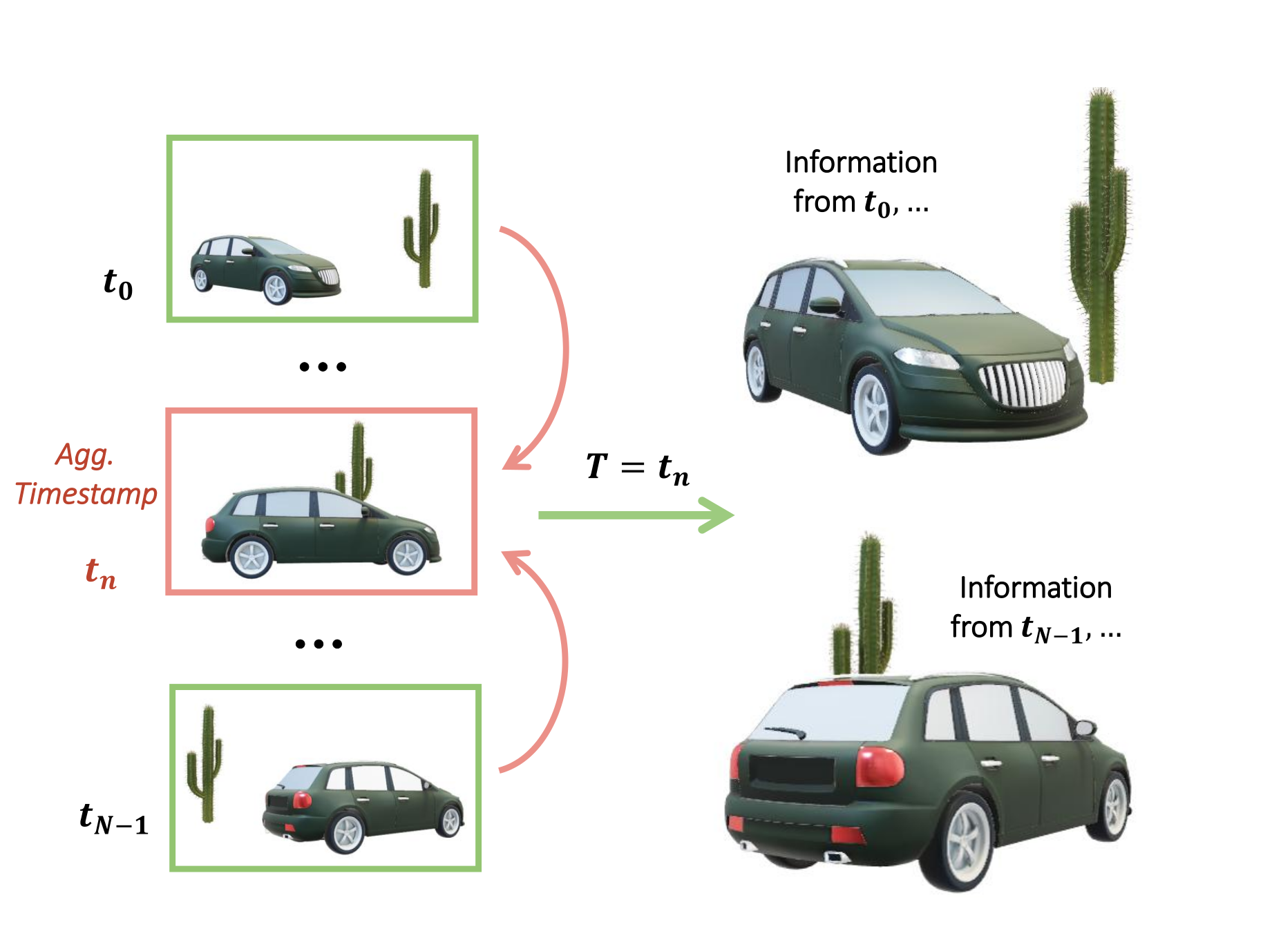
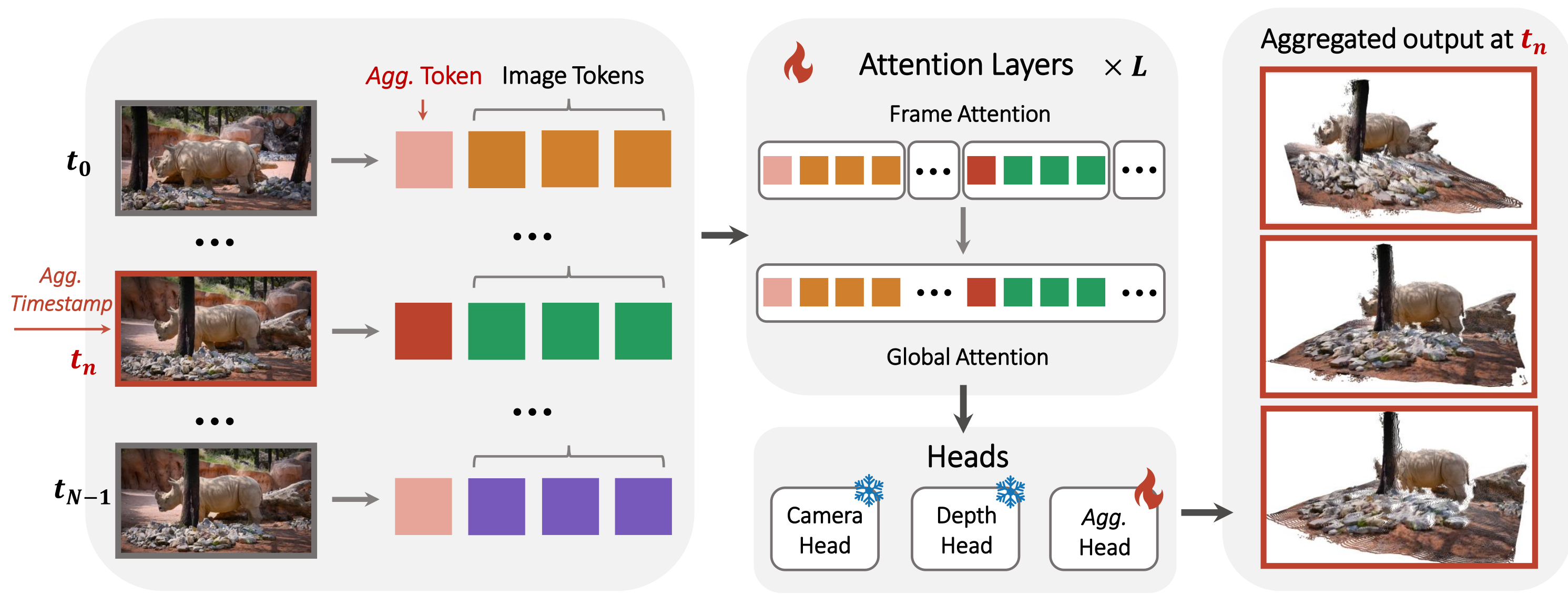
The task aligns points from static background and moving objects to a target time. The difficult case is a point visible in another frame but occluded at the target: its location must be inferred from the full sequence. Figures 2–3 retain the task illustration and complete architecture.
3.1 Task Formulation
The formulation distinguishes per-frame visible reconstruction, temporal completion and the trajectories obtained by changing the aggregation target.
Revisiting Prior Task Definitions.
Methods such as MonST3R primarily recover the point map visible at each timestamp. A moving object may reveal different parts over time, so these individually accurate maps can still omit its currently hidden surfaces.
Our Definition: Geometric Complete 4D Reconstruction.
Given N RGB frames and target a, predict a point map containing the observed surfaces from every frame in their configuration at a. All points remain grounded in some input observation; this differs from generating geometry unseen throughout the video.
The model uses past and future frames relative to a. Its global reconstruction is therefore an offline sequence operation, not a causal online predictor.
Equations
Relation to 3D Tracking.
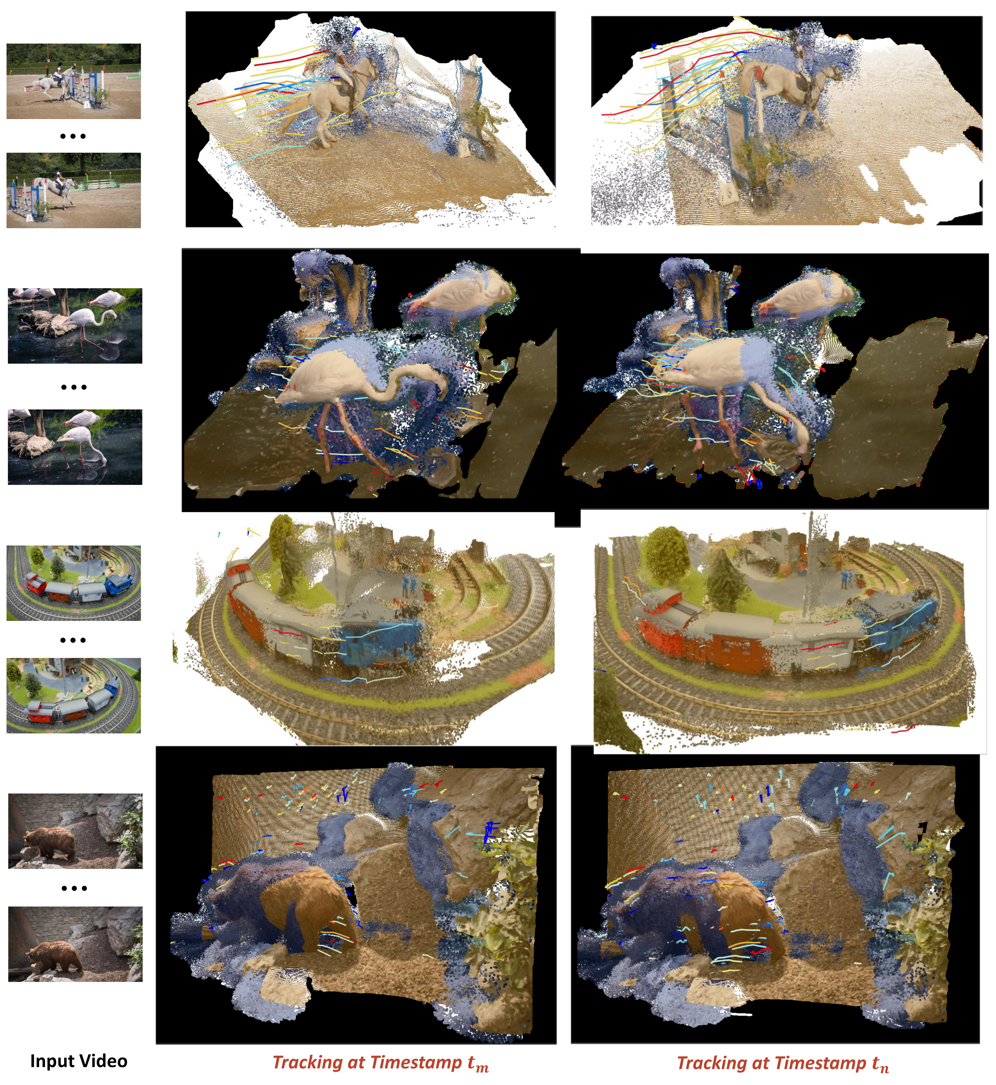
Run the same sequence with each frame as target. Corresponding source pixels then receive positions at successive times, producing dense 3D trajectories as a consequence of temporal aggregation. Continuity is learned from supervision rather than enforced by an explicit physical simulator.
3.2 Model Architecture
Equation 1 maps images and target a to one aggregated H×W×3 point map per source frame, nine camera parameters per frame, and H×W depth. DINOv2 embeds image patches into K visual tokens of width C.
The predicted geometry is expressed in a shared coordinate system anchored to the first frame. The target token selects a time configuration; it does not change that common coordinate reference.
Equations 1
| (1) |
Aggregation-aware Token Design.
Concatenate one aggregation-token set for the target frame and another shared set for all non-target frames. Changing the selected target directs the same network to gather geometry at another time.
Camera tokens predict pose/intrinsics. Following VGGT, separate first-frame registration tokens from the set shared by remaining frames to establish common coordinates. The ablation compares concatenation with adding aggregation tokens to image tokens.
Attention Mechanism.
Alternate within-frame and global self-attention. Aggregation tokens exchange information with visual tokens across the full sequence, including both past and future observations. This supports alignment of occluded surfaces without explicitly chaining adjacent-frame motion estimates.
Prediction Heads.
Keep VGGT’s camera and depth heads and replace its point head with an aggregation head. Depth and aggregation use DPT-style dense decoders; the camera head reads camera tokens. Each frame’s aggregation output supplies its observed points at the requested time, and their union forms the completed scene.
3.3 Training
Training combines aggregated-point, camera and depth supervision on synthetic dynamic sequences. The supplement retains the exact auxiliary losses and alternative point-weighting/representation formulas.
Training Losses.
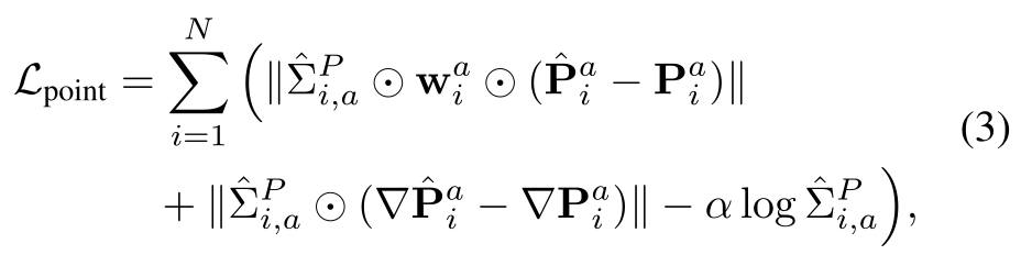
Equation 2 combines three losses. Focal weights increase with point-coordinate residual magnitude through scale β and exponent γ; equation 3 applies them to the point residual, alongside a spatial-gradient term and a negative log weighting penalty.
The predicted Σ map supplies learned aleatoric weighting, described as uncertainty in the source. Its multiplicative role should not be read as an independently calibrated uncertainty guarantee. Camera/depth supervision follows VGGT. The paper does not specify numerical λ, α, β or γ here.
Training Setup.
Initialize from VGGT, freeze the camera/depth heads and initialize aggregation from the original point head. The shared representation still changes, so frozen heads do not imply unchanged camera/depth predictions.
Train with AdamW for ten epochs, cosine learning rate peaking at 10⁻⁵, and the source’s stated “0.5-iteration warmup,” whose unit is unclear. Resize the long side to at most 518 pixels, sample width/height ratios 0.5–3.4, and use color jitter, Gaussian blur and grayscale. Training takes 23 hours on eight A100 GPUs.
Training Data.
Use 109 Point Odyssey, 483 Dynamic Replica and about 704 processed SAIL-VOS 3D sequences. They provide depth, camera and trajectory supervision.
For SAIL-VOS, locate each pixel barycentrically on a mesh triangle and follow vertex correspondences through time to generate 3D trajectories. Split long videos at large depth shifts associated with camera cuts. These synthetic training sets provide rich motion but do not establish broad real-world coverage.
4 Experiment
Evaluation separates dense 4D completion on a newly constructed SAIL-VOS subset from dynamic-point tracking on four datasets. Alignment choices and query selection matter for interpreting the reported gains.
| Acc. | Complet. | N.C. | ||||
|---|---|---|---|---|---|---|
| Methods | Mean | Med. | Mean | Med. | Mean | Med. |
| St4RTrack-seq | 0.92 | 0.71 | 3.10 | 0.17 | 0.48 | 0.47 |
| St4RTrack-pairs | 0.94 | 0.77 | 2.67 | 0.14 | 0.46 | 0.44 |
| Complet4R (Ours) | 0.50 | 0.37 | 0.26 | 0.11 | 0.49 | 0.49 |
4.1 4D Complete Reconstruction
Completion measures reconstructed-point accuracy, coverage of ground-truth geometry and normal consistency. All mean/median results and qualitative comparisons are retained.
Datasets.
The new test benchmark contains 44 SAIL-VOS 3D validation sequences with indoor/outdoor scenes and motion similar to training. It tests held-out sequences within a related synthetic distribution, rather than a diverse independent real-video completion benchmark.
Baselines.
Adapt two St4RTrack checkpoints, trained for sequence or pairwise prediction, by making every frame an anchor and accumulating the resulting tracked points. The comparison therefore tests this adaptation against a purpose-trained aggregation model.
Sparse trackers were excluded from this dense, occluded completion benchmark because the authors could not obtain suitable dense predictions under their hardware constraints. The baseline set is consequently limited.
Evaluation Metrics.
Follow CUT3R’s accuracy, completion and normal-consistency protocol. Randomly downsample both predicted and ground-truth points for evaluation. The text does not report the sampled point count or repeated-sampling uncertainty.
Results.
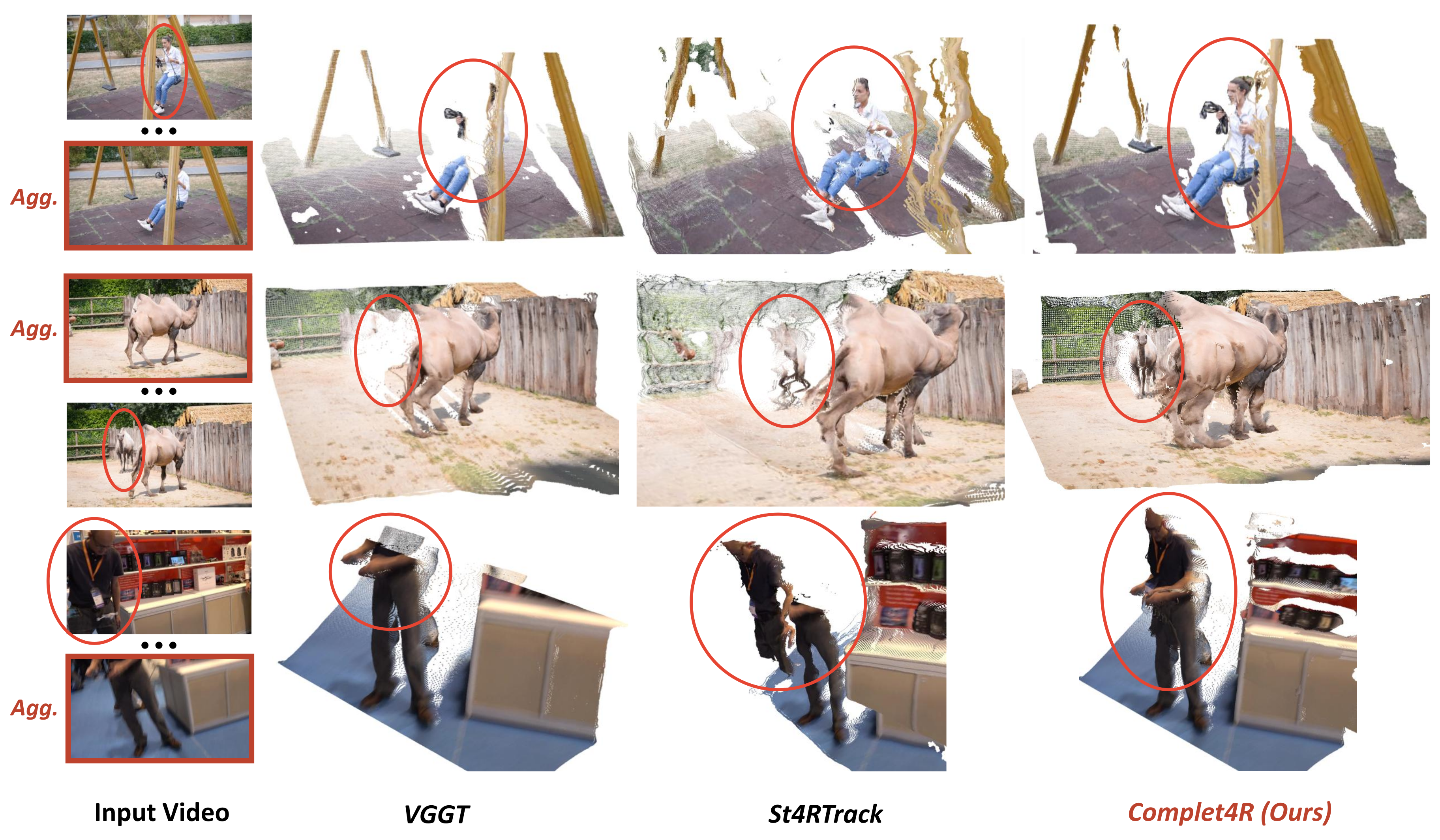
Table 1 gives mean accuracy error 0.50 versus 0.92/0.94 for the two St4RTrack variants, about a 46–47% reduction. Mean completion error falls from 3.10/2.67 to 0.26, while median completion improves more modestly from 0.17/0.14 to 0.11.
Mean normal consistency is 0.49 versus 0.48/0.46. Thus the largest relative gain is in mean coverage error, not an order-of-magnitude improvement in every metric. Figures 4 and 6 show selected occlusion and moving-object examples.
4.2 3D Point Tracking
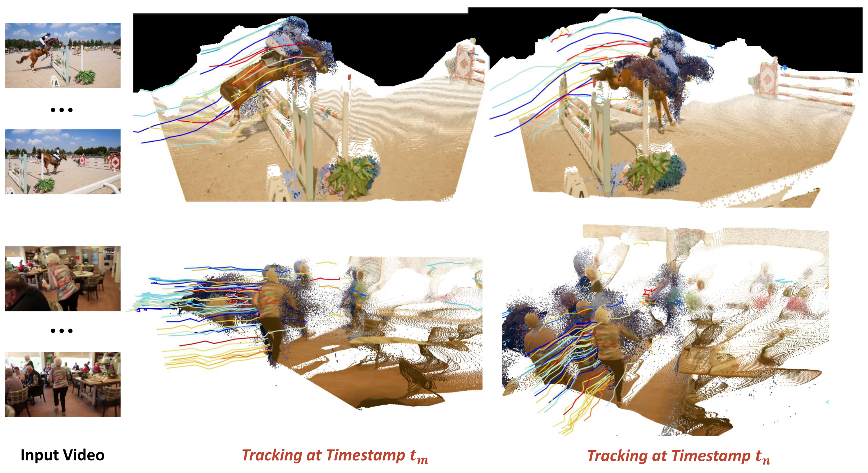
Changing the aggregation target produces world-coordinate 3D tracks without a separate tracking head. The main experiment evaluates dynamic points and uses ground-truth-assisted scale normalization.
| PO | DR | ADT | PStudio | ||||||
| Category | Methods | APD | EPE | APD | EPE | APD | EPE | APD | EPE |
| Combinational | SpaTracker+RANSAC-Procrustes | 53.77 | 43.58 | 58.58 | 104.44 | 66.49 | 16.00 | 52.05 | 42.66 |
| SpaTracker+MonST3R | 58.61 | 40.85 | 59.21 | 91.36 | 69.94 | 15.11 | 50.16 | 48.37 | |
| Feed-forward | MonST3R | 39.36 | 64.52 | 51.86 | 53.13 | 67.92 | 15.78 | 51.32 | 45.68 |
| SpaTracker | 51.20 | 46.95 | 58.65 | 108.28 | 67.65 | 16.28 | 62.59 | 30.94 | |
| St4RTrack | 68.72 | 29.70 | 68.13 | 29.61 | 75.34 | 12.12 | 69.67 | 26.37 | |
| Complet4R (Ours) | 80.17 | 16.07 | 80.65 | 15.99 | 77.34 | 9.72 | 76.88 | 18.52 | |
| Acc. | Complet. | N.C. | |||||||
|---|---|---|---|---|---|---|---|---|---|
| Variants | Loss | Agg. Repre. | Agg. Token | Mean | Med. | Mean | Med. | Mean | Med. |
| (1) | Dynamic | - | - | 0.50 | 0.47 | 0.26 | 0.20 | 0.48 | 0.47 |
| (2) | - | Offset | - | 0.63 | 0.42 | 0.50 | 0.11 | 0.44 | 0.40 |
| (3) | - | - | Add | 0.57 | 0.38 | 0.32 | 0.12 | 0.50 | 0.49 |
| Complet4R (Ours) | Focal | Endpoint | Concatenate | 0.50 | 0.37 | 0.26 | 0.11 | 0.49 | 0.49 |
Datasets and Baselines.
Use the WorldTrack protocol from St4RTrack on Point Odyssey, Dynamic Replica, Aria Digital Twin and Panoptic Studio. Select dynamic points visible in the first frame with complete ground-truth trajectories; this excludes initially hidden/newly appearing query points.
Compare feed-forward models and SpaTracker combined with RANSAC-Procrustes or MonST3R camera alignment. SpaTracker’s original output is not natively expressed in one unified world coordinate system.
Metric and Results.
First scale predictions by the ratio of median ground-truth and predicted point norms. APD averages the fractions within 0.1, 0.3, 0.5 and 1.0 m; EPE averages Euclidean trajectory error across frames. These are scale-aligned results, not absolute metric-scale recovery.
Complet4R’s APD is 80.17/80.65/77.34/76.88 across PO/DR/ADT/PStudio versus 68.72/68.13/75.34/69.67 for St4RTrack. Its printed EPE values are 16.07/15.99/9.72/18.52. The table does not label an EPE unit; avoid reading those printed magnitudes directly as meters. Selected smooth tracks are shown in Figures 5 and 8.
Equation
4.3 Ablation Study
Table 3 changes one component at a time: a fixed dynamic/static point weight replaces focal weighting; displacement replaces endpoint prediction; or addition replaces token concatenation. The default retains the best median accuracy and coverage, while some means tie and additive tokens slightly improve mean normal consistency (0.50 versus 0.49).
The evidence supports this combined design on the 44-sequence benchmark, without showing uniform superiority on every measure or variation across repeated training runs.
5 Conclusion
Complet4R makes temporal completion an explicit feed-forward task and obtains tracking through repeated target selection. Its strongest evidence is improved geometry and scale-aligned motion on the tested benchmarks.
Remaining limits include synthetic training, a small related-distribution completion test, global-attention cost, access to future frames and repeated target-conditioned predictions for a full timeline. Completion covers surfaces observed somewhere in the sequence; neither unseen-surface recovery nor strict elimination of drift is established. The abstract promises a code release but does not establish its availability.
6 Acknowledgements
The work acknowledges National Key R&D Program grant 2022ZD0161700 and the Tsinghua University Initiative Scientific Research Program.
7 Camera and Depth Supervision
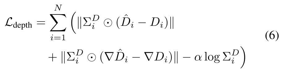
Equation 4 repeats the full objective. Camera supervision is a summed Huber loss over the nine-parameter camera representation (equation 5). Depth supervision uses learned per-pixel weighting on depth residuals and gradients plus a negative log penalty (equation 6), following VGGT.
The source’s exact symbols, subscripts and weighting conventions are retained. Camera/depth heads are frozen during training, but gradients can still update the common backbone through these objectives.
8 Details of the Ablation Study
The supplement gives the exact three alternatives used in Table 3, including the motion threshold that assigns dynamic-point weights and the displacement representation.
Dynamic-Weighted Point Loss.
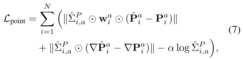
Replace focal weights with 1,000 for dynamic points and 1 for static points in the same uncertainty-weighted residual/gradient objective (equations 7–8). This alternative is based on motion labels rather than current prediction difficulty.
Compute each point’s displacement magnitude from the target across timestamps, then threshold the norm of that temporal displacement sequence (equations 9–10). Thresholds are 0.03 for Point Odyssey/Dynamic Replica and 0.01 for SAIL-VOS. The text does not specify a physical unit for these thresholds.
Aggregation Representation.
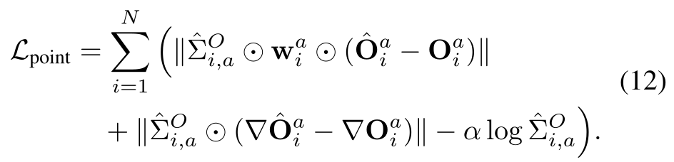
The default directly predicts each point’s target-time endpoint. The alternative predicts the offset from its position at another timestamp to the target (equation 11), with an analogous focal/gradient objective (equation 12).
Offset prediction raises mean accuracy error from 0.50 to 0.63 and completion error from 0.26 to 0.50 in Table 3. The original offset superscripts vary between definition and loss; the formulas are preserved without silently changing that notation.
| PO | DR | ADT | PStudio | ||||||
| Category | Methods | APD | EPE | APD | EPE | APD | EPE | APD | EPE |
| Combinational | SpaTracker+RANSAC-Procrustes | 61.00 | 33,38 | 61.65 | 37.20 | 88.65 | 5.96 | 67.82 | 26.60 |
| SpaTracker+MonST3R | 61.78 | 32.90 | 61.88 | 36.81 | 87.32 | 4.85 | 64.32 | 29.71 | |
| Feed-forward | MonST3R | 48.95 | 47.68 | 55.36 | 38.72 | 84.73 | 7.20 | 64.11 | 30.15 |
| SpaTracker | 60.49 | 33.74 | 61.32 | 37.50 | 87.68 | 6.16 | 80.76 | 16.50 | |
| St4RTrack | 67.43 | 28.70 | 67.90 | 26.27 | 85.34 | 6.88 | 76.97 | 19.69 | |
| Complet4R (Ours) | 85.82 | 12.39 | 85.30 | 12.78 | 87.58 | 5.39 | 85.62 | 12.49 | |
Aggregation Tokens.
Compare concatenating the aggregation tokens with adding them to image tokens. Concatenation gives lower accuracy/coverage errors overall, while mean normal consistency favors addition slightly. This ablation does not isolate how token count or compute contributes.
9 Additional Experiments
Additional experiments test tracking after a richer similarity alignment, retained camera/depth prediction, and sequence-length runtime and memory.
9.1 Additional 3D Point Tracking Evaluation
Global SIM(3) aligns rotation, translation and scale to ground truth before tracking evaluation. Complet4R leads both reported metrics on PO, DR and PStudio, but not ADT: APD 87.58 trails SpaTracker+RANSAC-Procrustes at 88.65, and EPE 5.39 trails SpaTracker+MonST3R at 4.85.
The stronger alignment removes additional global errors and differs from the main median-scale protocol. Table 4’s printed “33,38” is retained as supplied rather than silently corrected.
9.2 Depth and Camera Pose Estimation
Depth results on Sintel, BONN and KITTI fall between VGGT and CUT3R on every listed metric. For example, Sintel Abs Rel is 0.353 versus 0.298/0.421. This indicates useful retained depth ability, not preservation of the pretrained model’s best performance.
Camera pose degrades more: on Sintel, all Complet4R errors exceed both baselines; on ScanNet, it improves ATE/rotation over CUT3R but has slightly worse translation error. VGGT leads all camera columns. Frozen output heads do not prevent these changes after shared-backbone fine-tuning.
9.3 Runtime and Memory
On one A100 at 294×518 input resolution, 16/64/256 frames require 0.51/2.95/27.86 seconds and 10.2/15.1/28.6 GB. Runtime rises nonlinearly because of global attention. FlashAttention is suggested as future optimization, not evaluated here.
The table reports processing by input length without specifying the total cost of repeating every target timestamp. Its single-call timing should not automatically be interpreted as the cost of reconstructing a complete N-target timeline.
10 Additional Qualitative Results
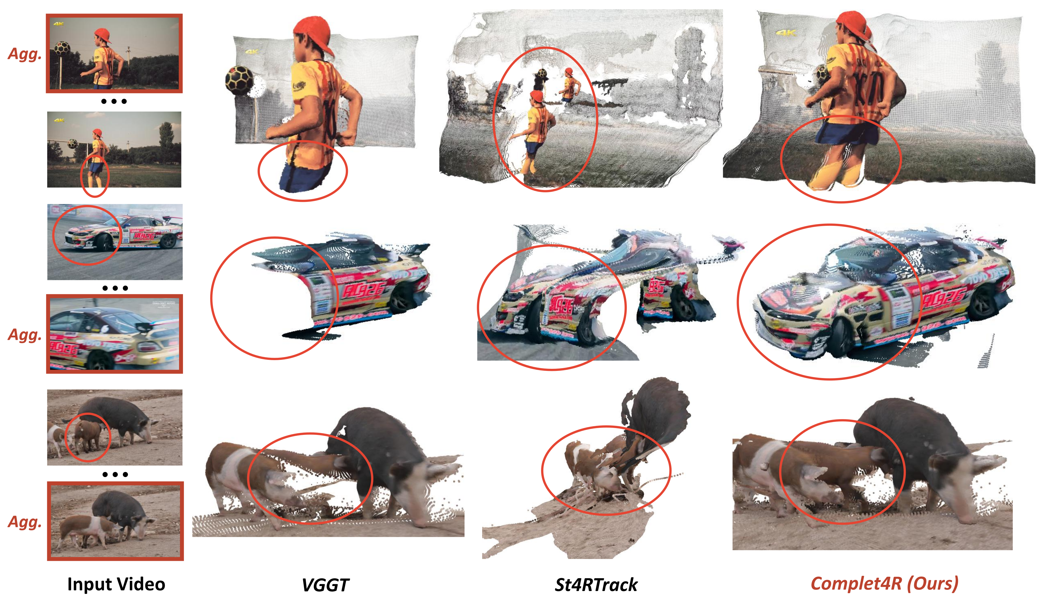
Figure 6 retains further selected dense-completion examples. Moving people, vehicles and animals illustrate the intended recovery of currently hidden geometry from other observations. Qualitative examples complement the benchmark rather than quantify failure frequency.
11 Additional Discussion
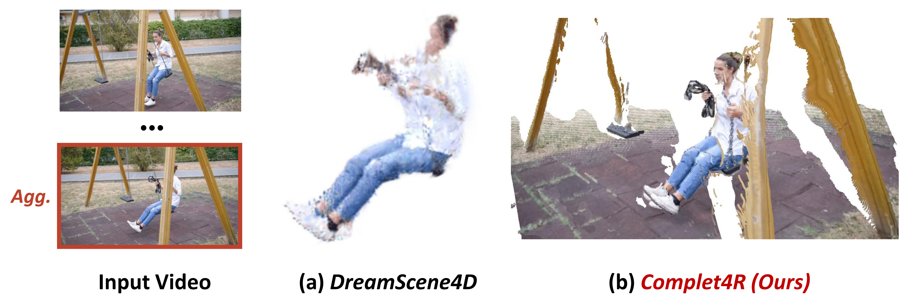
Figure 7 compares geometry with DreamScene4D, a diffusion-based per-scene reconstruction method aimed partly at photorealistic rendering. The selected example favors Complet4R’s shape and consistency; Figure 8 retains additional dynamic tracks.
The paper reports roughly 0.5 seconds versus 28 minutes for a sixteen-frame sequence. Different output goals and optimization procedures qualify that comparison: this is not a matched photorealistic novel-view benchmark, nor evidence that every sequence or complete target timeline has the same speedup.