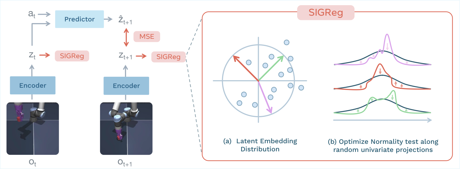
The training and planning diagrams distinguish the learned encoder/predictor from the cross-entropy optimizer used only at deployment.
Figure 1: LeWorldModel Training Pipeline. Given frame observations and actions , the encoder maps frames into low-dimensional latent representations . The predictor models the environment dynamics by autoregressively predicting the next latent state from the current latent state and action . The encoder and predictor are jointly optimized using a mean-squared error (MSE) prediction loss. LeWM does not rely on any training heuristics, such as stop-gradient, exponential moving averages, or pre-trained representations. To prevent trivial collapse, the SIGReg regularization term enforces Gaussian-distributed latent embeddings, promoting feature diversity. For tractability, latent embeddings are projected onto multiple random directions, and a normality test is applied to each one-dimensional projection. Aggregating these statistics encourages the full embedding distribution to match an isotropic Gaussian.
At a glance
Intuition. A compact world model should remember enough about a scene to predict what an action will change, while ignoring unnecessary image detail. Predicting its own learned representations creates a trap: every image could map to the same constant. LeWorldModel pairs next-latent prediction with SIGReg, which encourages a diverse, approximately isotropic Gaussian representation distribution. It trains the visual encoder and action-conditioned predictor together from pixels, without rewards, pixel reconstruction, a frozen foundation encoder, or an EMA teacher. A roughly 15-million-parameter model supports rapid simulated control and physical-variable probing. Its reported 48-fold planning speedup is tied to the chosen foundation-model baseline and planning settings; it is not a universal speedup or a guarantee that all task-relevant physical information survives.
1 Introduction
The work simplifies end-to-end JEPA world-model training to a prediction term and one anti-collapse regularizer. Compact global state vectors reduce the cost of repeatedly imagining candidate actions. The contribution combines a practical training recipe with control, probing and surprise evaluations, rather than claiming that low prediction loss alone proves physical understanding.
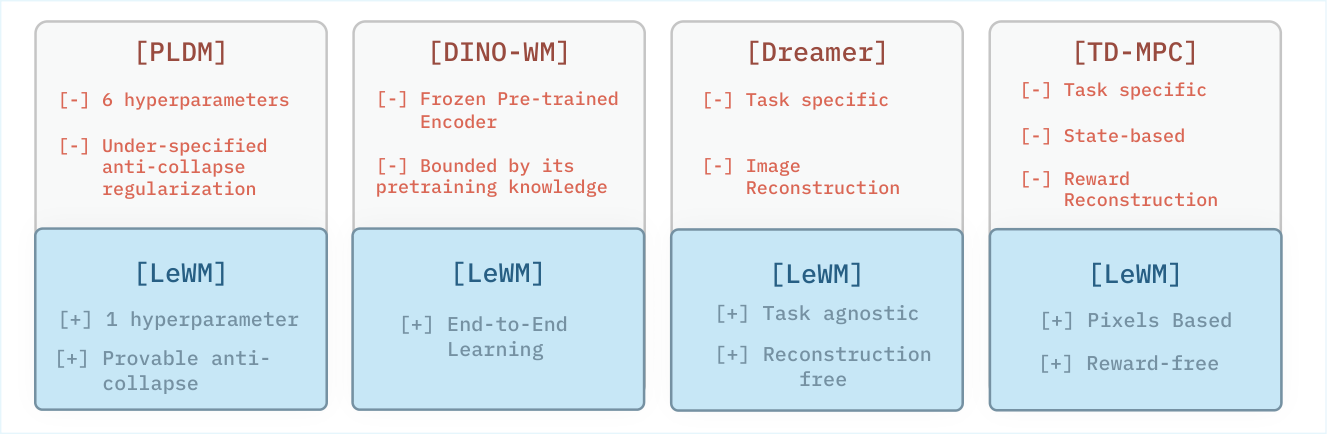
Figure 2: Characteristics of latent world model approaches. Methods are grouped by training paradigm. End-to-end methods (PLDM) learn the encoder and predictor jointly from pixels without pre-trained representations or heuristics like stop-gradient or EMAs, but require many hyperparameters and lack collapse guarantees. Foundation-based methods (DINO-WM) avoid collapse by freezing a pre-trained vision encoder, forgoing end-to-end learning. Task-specific methods (Dreamer, TD-MPC) require reward signals or privileged state access. LeWM combines the strengths of all three: end-to-end, task-agnostic, pixel-based, reconstruction- and reward-free, with a single hyperparameter with provable anti-collapse guarantees.
2 Related Work
The paper distinguishes generative simulators, frozen-feature latent models, and end-to-end latent models. Generative approaches reconstruct more visual detail and may use rewards; frozen encoders inherit a representation learned elsewhere. LeWorldModel instead learns a reward-free control representation jointly with its dynamics predictor, accepting the resulting collapse-prevention problem.
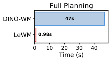
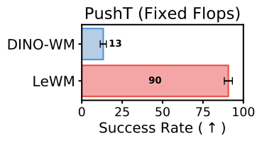
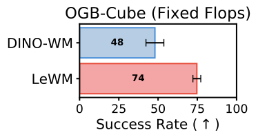
Figure 3: Planning time and performance under fixed compute.Left: Planning time comparison averaged over 50 runs. Encoding observations with fewer tokens than DINO-WM allows LeWM to achieve planning speeds comparable to PLDM while being up to faster than DINO-WM.
Center–Right: Planning performance under the same computational budget (fixed FLOPs). LeWM significantly outperforms DINO-WM on Push-T (center) and OGBench-Cube (right). See App. D for planning setup details.
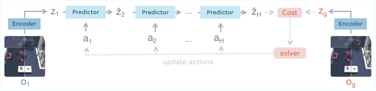
Figure 4: Latent Planning with LeWorldModel . Given an initial observation and a goal , the world model learned in Fig. 2 performs planning in the LeWM latent space. The initial state embedding and the goal embedding are obtained from the encoder. The predictor then rolls out future latent states up to a horizon . A latent cost between the final predicted state and the goal embedding guides a solver to optimize the action sequence. This prediction–optimization loop is repeated until convergence to a good plan candidate.
3 Method: LeWorldModel
Training learns the encoder and predictor from offline action–observation trajectories. Deployment freezes them and searches for actions that bring the predicted latent state near an encoded goal.
3.1 Learning the Latent World Model
Offline Dataset.
The data contains observations and actions but no task rewards or optimality labels. Coverage of relevant transitions still matters: reward-free training does not remove the need for informative interaction data.
Model Architecture.
A small vision transformer produces a projected global state vector, and a causal transformer predicts its successor from recent states and actions. Adaptive layer normalization injects actions into the predictor. Projection after normalization is important for allowing the Gaussian-distribution objective to operate on the learned representation.
Teacher-forced latent prediction encourages temporal predictability; SIGReg discourages a constant representation by testing random one-dimensional projections against a Gaussian reference. A single weight balances these terms. Finite random projections and empirical optimization approximate the distributional target; they do not prove exact Gaussianity or preservation of every physical factor.
Equations 1–3
(1)
(2)
(3)
3.2 Latent Planning
Cross-entropy search optimizes candidate action sequences under a terminal latent-goal cost. Only an initial action segment is executed before replanning from a new observation. This receding horizon limits the practical effect of accumulated model error without eliminating it.
Equations 4–5
(4)
(5)
4 Latent Planning Performance
4.1 Planning evaluation setup
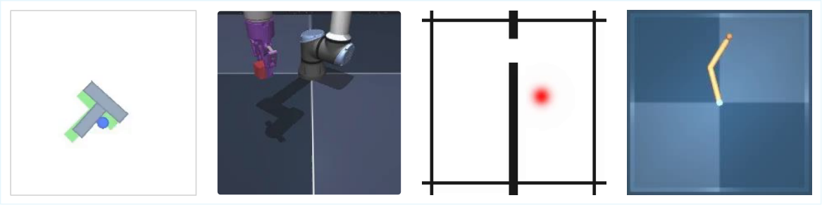
Figure 5: Environments used for evaluation. Left: Push-T, a 2D manipulation task where the agent must push a block toward a target configuration, commonly used as a robotics benchmark. Center (1): OGBench-Cube, a visually richer 3D manipulation environment where a robotic arm interacts with a cube to reach a target position. Center (2): Two-Room, a simple 2D navigation environment where an agent moves between rooms to reach target positions. Right: Reacher, a task where a 2-joint arm needs to reach a target configuration in a 2D plane. All environments have a continuous action space. More details on environment and datasets are available in appendix E.
Environments.
The simulations span navigation, arm motion and contact-rich manipulation in two and three dimensions. They test controlled settings with offline data, not open-world real-robot generalization.
Baselines.
PLDM is the closest end-to-end latent baseline; DINO-WM uses a pretrained visual encoder and many patch features. Goal-conditioned behavioral cloning and offline value-learning baselines supply policy-based comparisons. Proprioception is controlled where specified because extra state information changes the problem.
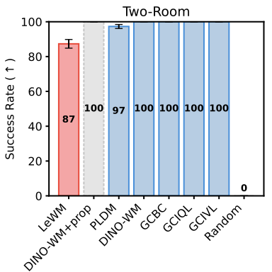
LeWorldModel improves several difficult tasks over PLDM and is competitive with DINO-WM while planning much faster in the reported configuration. It is worse on Two-Room. The suggested explanation—low dataset complexity conflicting with a high-dimensional Gaussian target—is plausible but not isolated as a universal cause.
4.3 Towards Stable Training of World Models
Ablations.
Projection count, representation dimension and architecture are ablated. Performance often saturates across a useful range, while the regularization weight remains consequential. Fewer tuned loss coefficients simplify experimentation; the paper’s search-complexity comparison should not be read as a general theorem that tuning one parameter is logarithmic.
Training Curves.
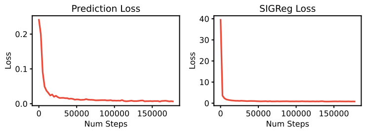
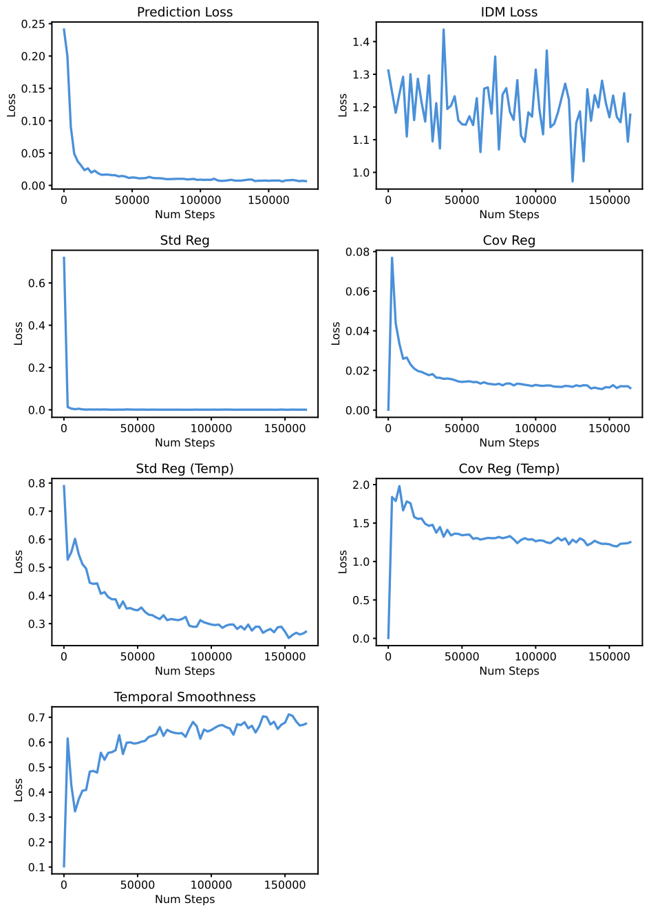
The displayed training curves are smoother for this two-term recipe than the compared multi-term PLDM run. Smooth optimization traces support the empirical stability claim for these settings, not a guarantee across arbitrary datasets and seeds.
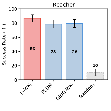
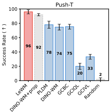
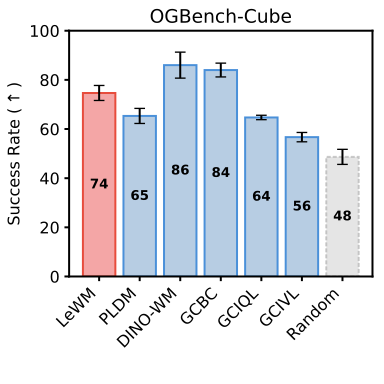
Figure 6: Planning performance across environments.
Results are shown for Two-Room (left), Reacher (center 1), PushT (center-2) and OGBench-Cube (right).
LeWM consistently outperforms PLDM and DINO-WM on Push-T and Reacher. On OGBench-Cube, DINO-WM slightly outperforms LeWM, possibly due to the higher visual complexity and the 3D nature of the environment, which makes encoder training more challenging. In the simpler Two-Room environment, PLDM and DINO-WM outperform LeWM, which may be explained by the SIGReg regularization encouraging a Gaussian distribution in a high-dimensional latent space, while the intrinsic dimensionality of the environment is much lower.
Three diagnostics probe what the latent model retains: predicting physical variables, decoding visualizations, and detecting unexpected changes. They measure different properties and do not independently establish an identified physical state model.
5.1 Physical Structure of the Latent Space
Probing physical quantities.
Supervised linear and nonlinear probes predict physical quantities from frozen latents. Competitive probing means the information is recoverable by those probes; it does not prove that the planning procedure actually uses it.
Table 1: Physical latent probing results on Push-T.LeWM consistently
outperforms PLDM while remaining competitive with DINO-WM. The strong probing
performance of DINO-WM on certain properties may stem from its foundation-model
pretraining: the DINOv2 encoder is trained on two orders of magnitude more data
(124M images) spanning a far more diverse
distribution, which likely allows it to capture some physical properties in its
embeddings by default.
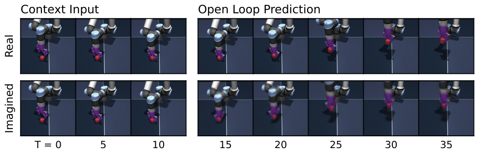
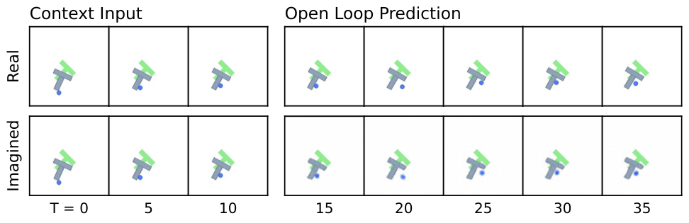
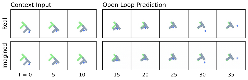
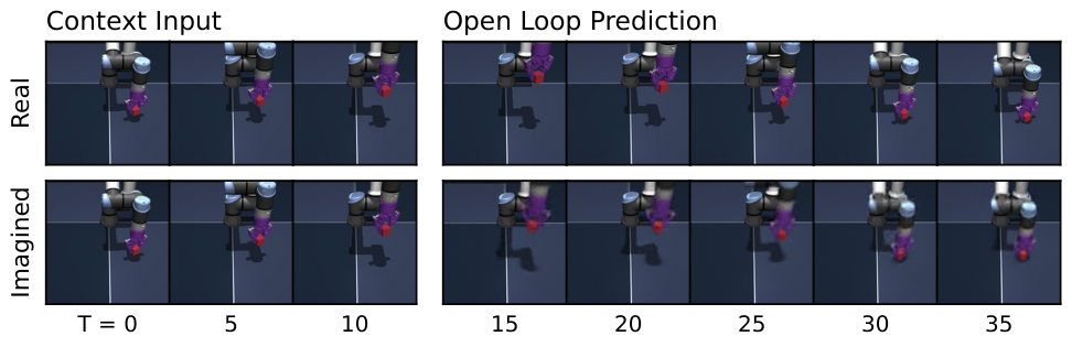
Figure 7: Predictor rollout on OGBench-Cube. We visualize decoded latent plans from LeWM given context and action sequences. Each rollout encodes three image observations as context, then autoregressively generates future latents conditioned on the actions in an open-loop fashion. Latents are decoded via a decoder trained a posteriori. The imagined rollout suggests that latent representations capture the global scene structure while finer details like end-effector angle are not fully preserved. Additional rollouts for Push-T and OGBench-Cube are provided in Fig. 9.
Decoding Latent Space.
A separate visualization decoder reconstructs observations from frozen representations. Reconstruction is not part of world-model training. The decoded images reveal retained information and prediction errors without changing the control model.
Visualizing Latent Space.
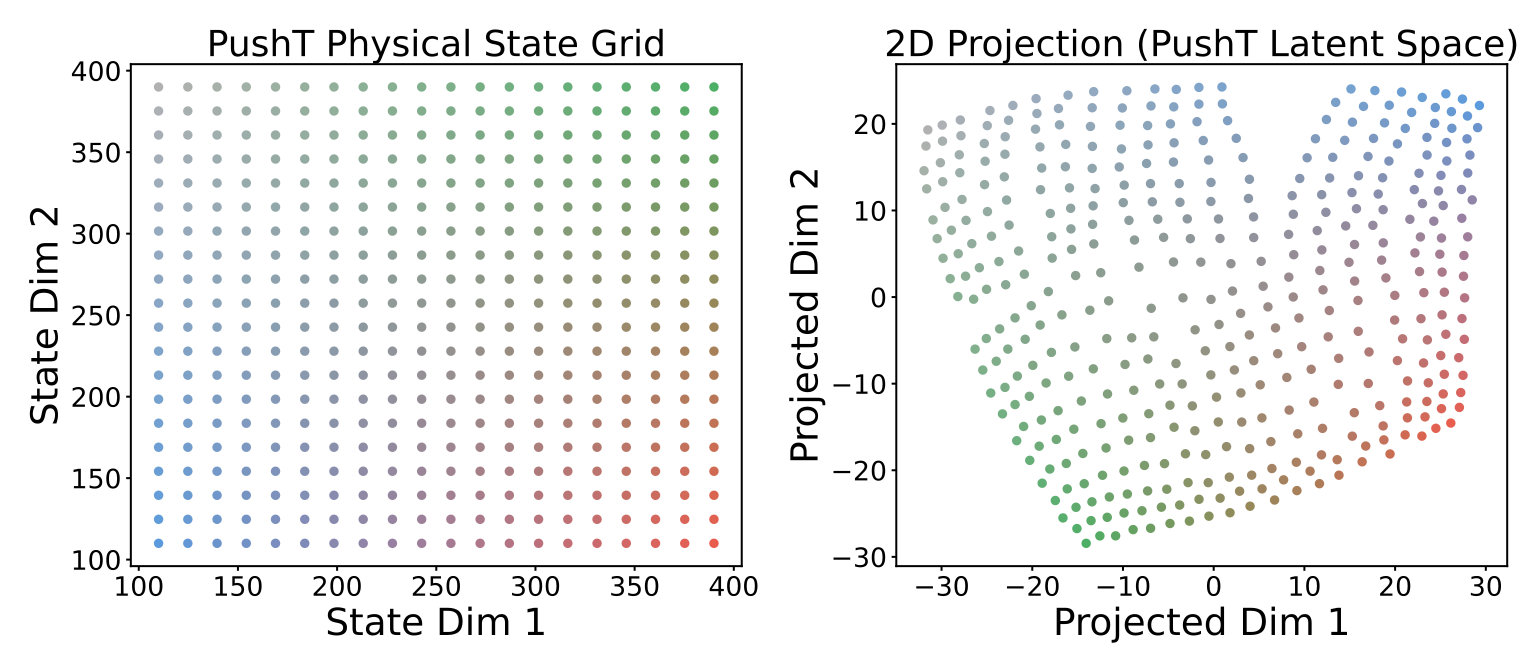
A t-SNE plot visually relates latent neighborhoods to positions in Push-T. This is a qualitative projection, whose appearance cannot by itself establish a globally faithful or Euclidean physical geometry.
Temporal Latent Path Straightening.
Consecutive latent velocity vectors become more aligned during training on the studied trajectories. This temporal straightening is observed without a dedicated smoothness term. It is a descriptive statistic and does not imply globally straight optimal routes around obstacles.
5.2 Violation-of-expectation Framework
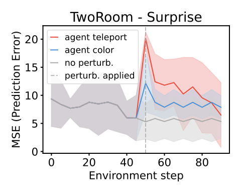
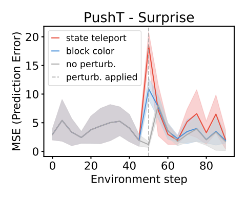
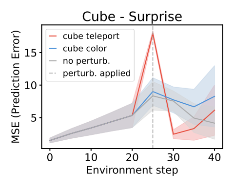
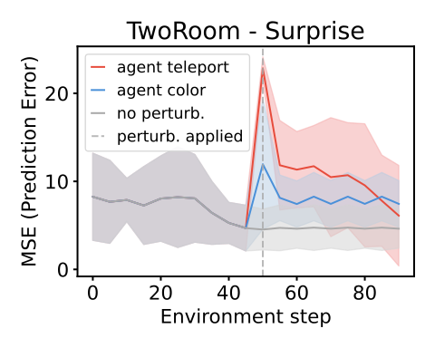
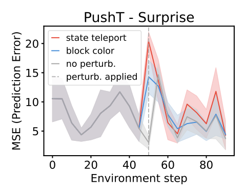
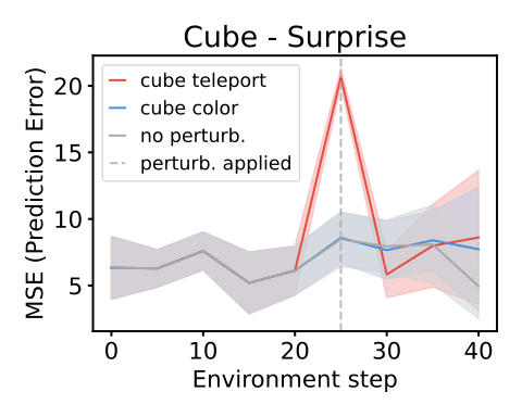
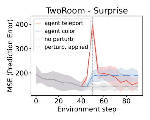
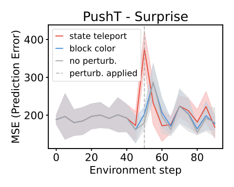
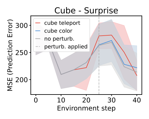
Surprise is prediction discrepancy on perturbed trajectories. Physical changes are compared with cosmetic color changes and unperturbed controls. Higher response to the former suggests sensitivity to learned dynamics; the designed perturbations remain a limited test of general physical reasoning.
Figure 8: Violation-of-expectation evaluation across three environments. Each plot shows LeWM surprise along three trajectories: an unperturbed reference, a visually perturbed trajectory with abrupt object color change, and a physically perturbed trajectory where objects teleport to random positions. Teleportation violates physical continuity and produces a pronounced surprise spike, while the unperturbed trajectory stays at a low baseline. The increase is significant for teleportation across all environments (paired t-test, ) but weaker and non-significant for color changes, indicating greater sensitivity to physical than visual perturbations. Environments, left to right: TwoRoom, PushT, OGBench Cube.
6 Conclusion
A small end-to-end representation can be useful for fast latent-space control with a simpler objective than the compared recipe. The paper’s practical evidence combines planning performance and diagnostic probes; broader generalization and representation guarantees remain open.
Limitations & Future Work.
The tested domains are relatively controlled, and low-complexity data can challenge the Gaussian target. Future work includes larger and more diverse settings and extensions beyond the evaluated control tasks.
SIGReg evaluates random scalar projections of embeddings using an Epps–Pulley normality statistic. Matching all projections has a distributional justification, but the implementation uses finitely many sampled directions and integration points. The appendix preserves the exact statistic and training pseudocode.
Cross-entropy planning iteratively samples actions, scores predicted endpoints, and updates the candidate distribution from elites. Planning hyperparameters and replanning frequency are part of the efficiency/accuracy comparison.
Algorithm 2 Cross-Entropy Method (CEM) for Action Sequence Optimization
1:
World model , planning horizon , number of samples , number of elites , number of iterations
2:
Initialize sampling distribution parameters ,
3:for to do
4:
Sample candidate action sequences
5:for to do
6:
Roll out in the world model
7:
Compute cost
8:endfor
9:
Select the sequences with lowest cost (elites)
10:
Update distribution parameters using elite set:
11:
12:
13:endfor
14:return best action sequence found or first action of
DINO-WM predicts frozen pretrained patch features. Its larger token set increases planning cost and can preserve detail absent from a small global vector, so speed and information content should be compared together.
PLDM learns perception and dynamics jointly with several variance, covariance, temporal and related regularization terms. Its coefficient search and architecture are specified to make the end-to-end baseline reproducible rather than assuming all such methods share one stability profile.
Goal-conditioned offline reinforcement learning learns value information and an action-selection mechanism from fixed trajectories. It is a distinct route to control from optimizing an action sequence through a predictive model.
Goal-conditioned implicit Q-learning uses expectile-based value fitting on offline transitions. Its learned policy extraction and value assumptions differ from the latent endpoint-matching cost used by LeWorldModel.
The alternative goal-conditioned value-learning baseline changes how the value is estimated. The appendix preserves that objective rather than treating every offline value method as the same comparator.
Equation
Policy extraction.
A policy is extracted from the fitted goal-conditioned value representation. Its deployment avoids repeated world-model rollout but inherits the offline data and value-learning limitations.
Goal-conditioned behavioral cloning predicts dataset actions conditioned on goals. This baseline directly learns behavior instead of modeling dynamics; its performance depends on how useful the observed trajectories are for the evaluation goals.
Equation
Appendix D Implementation details
Implementation details retain the model architectures, optimization settings and planning configuration needed to distinguish representation compactness from other recipe changes.
Figure 9: Algorithm 9. Pseudo-code for the training procedure of LeWorldModel. Pixel observations are encoded into latent embeddings, and a predictor estimates the dynamics by predicting the next-step embedding conditioned on actions. The model is optimized end-to-end using a next-embedding prediction loss together with a step-wise SIGReg regularization term to prevent representation collapse.
Encoder Architecture.
The visual encoder uses the specified small transformer and projected global token. This bottleneck is central to fast rollout computation.
Predictor Architecture.
The causal transformer predictor combines recent latent states with action conditioning. It forecasts latent state rather than pixels.
Decoder (Visualization Only).
The separately trained decoder is used only to inspect reconstructions and imagined futures. It contributes no reconstruction loss to the learned dynamics representation.
Planning solver.
Candidate counts, elite selection, horizon and executed-action chunk specify the cross-entropy solver. Changing them changes both runtime and control success.
Appendix E Environment & Dataset
Environment descriptions explain dataset generation, action spaces and observations for Two-Room, Reacher, Push-T and OGBench Cube. Dataset diversity and complexity differ across tasks, limiting a single interpretation of all gains and failures.
Appendix F Evaluation Details
Figure 9: Additional predictor rollouts on PushT (top) and OGBench-Cube (bottom). Same setup as Fig. 7: three context frames are encoded into latent representations, and the predictor autoregressively generates future latent states conditioned on the action sequence. All predictions are decoded using a decoder not used during training. On PushT, the imagined trajectory closely tracks the real one, accurately capturing both agent and block motion. On OGBench-Cube, the model preserves the overall scene layout and cube displacement but loses finer details such as end-effector orientation at longer horizons, consistent with the lower probing accuracy on rotational quantities reported in Tab. 4.
F.1 Control
Control evaluation fixes the initial–goal tasks and success definitions, with matched planning settings where specified. A task-specific success rate is more informative about control than prediction error alone.
F.2 Probing
Probe data and supervised targets are separated from representation training. The retained tables distinguish positional, velocity and other physical quantities rather than reducing them to one aggregate score.
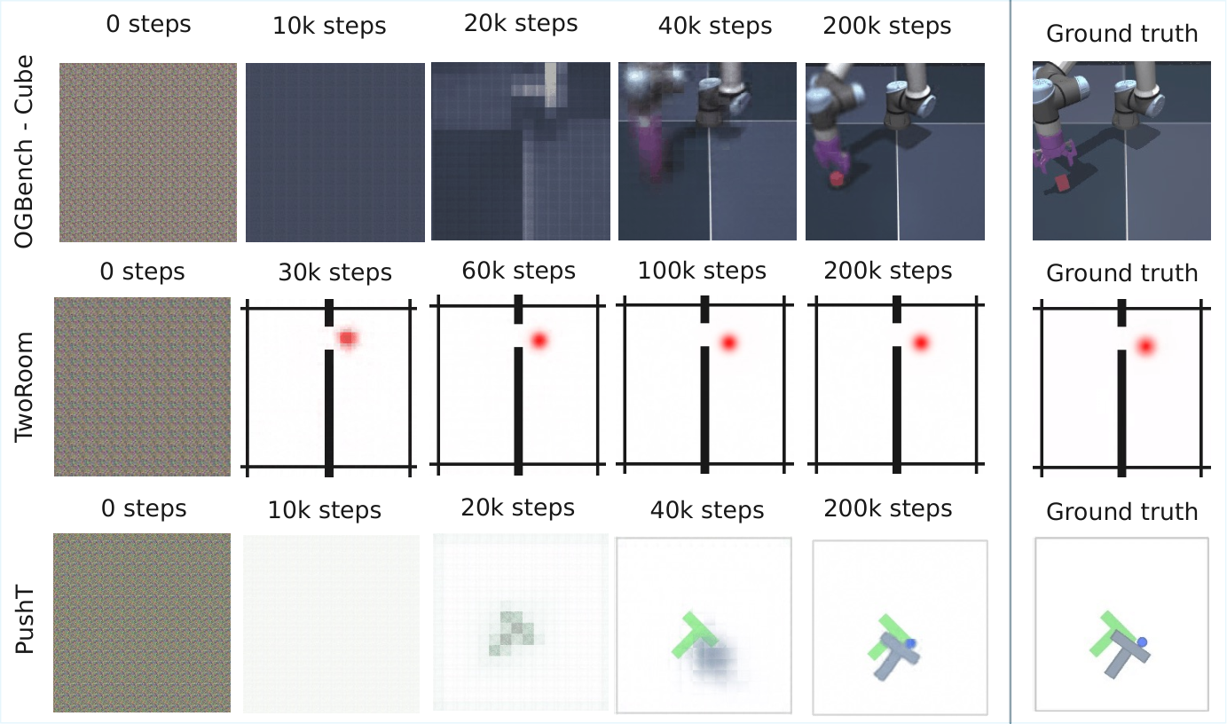
Figure 10: Decoder visualization during training. As training progresses, the latent representation increasingly captures the information required to reconstruct the visual scene, even though no reconstruction loss is used during training. Early in training, the decoded images correspond to slow features, a phenomenon previously reported [46].
Table 3: Physical Latent Probing results on TwoRoom. Although LeWM underperforms PLDM in downstream planning on this environment, it matches or outperforms PLDM across all probing metrics, and both methods substantially outperform DINO-WM on the linear probe. This suggests that the learned latent space captures the underlying physical state equally well and that the planning gap is not due to a less informative representation but rather to other factors such as the dynamics model or the planning procedure itself.
Table 4: Physical latent probing results on OGBench-Cube.LeWM matches or outperforms PLDM on most properties and achieves the best results on positional quantities such as block position and end-effector position. DINO-WM retains a clear advantage on dynamic and rotational properties (joint velocity, end-effector yaw), likely because such quantities benefit from the richer visual priors learned during large-scale pretraining. All three methods struggle to recover block orientation (quaternion and yaw), suggesting that fine-grained rotational information remains difficult to encode in compact latent spaces
regardless of the training strategy.
The surprise protocol inserts controlled visual or physical changes into otherwise comparable trajectories. The examples and discrepancy curves show both the timing and type of detected perturbation.
TwoRoom.
Two-Room perturbations test whether the model responds differently to cosmetic changes and changes affecting navigation dynamics. The environment’s simplicity also contributes to its special behavior elsewhere in the study.
PushT.
Push-T perturbs the manipulation scene and compares surprise against unperturbed motion. These tests target the learned relation between action and object motion.
OGBench-Cube.
Cube experiments extend the same logic to three-dimensional manipulation. Their controlled violations do not cover every possible visual distraction or physical change.
Figure 11: Example of trajectories used for the Violation of Expectation experiments (Sec. 5.2). For each environment, the first row corresponds to the unperturbed trajectory, the second row corresponds to a trajectory where a visual perturbation occurs and the third row displays trajectories where the state of the system is randomly reset in the middle of the trajectory. The frame where the perturbation occurs is highlighted in red.
Figure 12: Violation-of-expectation evaluation with PLDM. From left to right: TwoRoom, PushT, and OGBench-Cube. Surprise is plotted over time for unperturbed, visually perturbed, and physically perturbed trajectories. In TwoRoom and PushT, the model assigns significantly higher surprise to both visual and physical perturbations. In OGBench-Cube, the increase in surprise is weaker and not consistently significant.Figure 13: Visualization of the latent space obtained with LeWM for the PushT environment. On the left, the grid of states is obtained by moving the agent and the block in the x-y plane. On the right, the embeddings of these states are visualized using a t-SNE.
Figure 14: Violation-of-expectation evaluation with DINO-WM. From left to right: TwoRoom, PushT, and OGBench-Cube. Surprise is plotted over time for unperturbed, visually perturbed, and physically perturbed trajectories. While the model detects both perturbations in TwoRoom and PushT, surprise does not increase significantly for either perturbation in OGBench-Cube.
Appendix G Ablations.
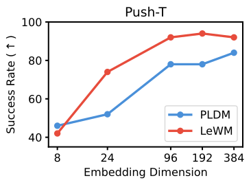
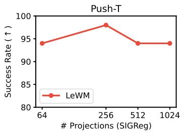
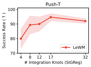
Figure 15: Ablation studies of key design choices in LeWM.Left: effect of the embedding dimension; performance improves with larger embeddings but quickly saturates beyond a certain threshold. Center: effect of the number of random projections used in SIGReg; performance remains stable, indicating that this parameter is not critical. Right: effect of the number of integration knots used to compute the SIGReg loss; results are similarly insensitive to this parameter.
Training variance.
Training-seed variation checks whether the reported behavior depends on one initialization. The measured variation is specific to these tasks and budgets.
Table 5: Training Variance. We report the mean success rate across three training seeds and the corresponding variance, evaluated over the same set of 50 trajectories on Push-T. The goal configuration is reachable within 25 steps, and we allow a planning budget of 50 steps. PLDM exhibits higher variance compared to DINO-WM and LeWM.
Too small a bottleneck loses useful state information; larger dimensions eventually provide diminishing benefit. Capacity therefore remains a real design choice even with a simpler loss.
The projection-count ablation tests the cost and adequacy of the sampled Gaussian tests. Empirical robustness over tested counts does not make a finite test exact.
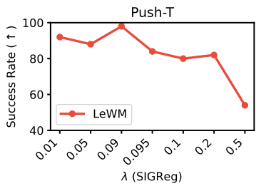
The balance between prediction and regularization is tuned. Too little regularization risks collapse; too much can prioritize the distributional target over task-relevant predictability.
Figure 16: Effect of the SIGReg regularization weight on Push-T planning performance. Success rate remains above 80% across a wide range of values (), peaking near . Performance degrades sharply only at , where the regularizer dominates the prediction loss and hinders dynamics modeling. Since is the only effective hyperparameter of LeWM, the SIGReg loss coefficient is easy to tune via a simple bisection search.
Predictor Size.
Predictor capacity affects dynamics quality and planning cost. The retained comparison separates that choice from encoder dimension.
Table 6: Effect of the predictor size on planning performance in the Push-T environment. We report the success rate (SR). The ViT-S predictor achieves the best performance.
A decoder is evaluated as an auxiliary design choice. The final claim about a reconstruction-free training recipe should be read against this explicit ablation.
Table 7: Effect of adding a reconstruction loss during training. We report the success rate (SR) on the Push-T planning task. The model trained without the decoder loss achieves higher performance.
A residual convolutional encoder supplies an architectural control. Competitive results suggest the recipe is not limited to the default transformer, within the examined settings.
Table 8: Encoder Architecture Effect. We report the success rate (SR) on the Push-T planning task. LeWM achieves competitive performance across encoder architectures, with ViT holding a slight edge.
Predictor dropout is varied to assess its contribution to generalization and optimization. The selected rate remains a recipe choice, not a mathematical requirement of JEPA.
Table 9: Effect of predictor dropout during training on Push-T planning performance. We report the success rate (SR). A small amount of dropout () yields the best results.
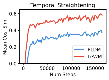
Temporal straightness is measured by alignment of successive latent differences, with controls against alternative models. The statistic tracks a training-time geometric trend; it is neither a route-length metric nor a theorem about all latent trajectories.
Equation 9
(9)
Figure 17: Temporal Latent Straightening on Push-T. Mean cosine similarity between consecutive latent velocity vectors (Eq. 9) over training. Higher values indicate straighter latent trajectories. PLDM explicitly encourages temporal regularity through a dedicated temporal smoothness loss (), yet LeWM achieves substantially straighter latent paths as a purely emergent phenomenon, without any temporal regularization term in its objective.
Appendix I Training Curves
Complete loss traces retain both prediction and anti-collapse components for the compared models. They support a qualitative stability comparison under the stated runs and hyperparameters.
Figure 18: Push-T Training curves for LeWM.Figure 19: Push-T Training curves for PLDM.
51 references
[1]E. Alonso, A. Jelley, V. Micheli, A. Kanervisto, A. Storkey, T. Pearce, and F. Fleuret (2024)Diffusion for world modeling: visual details matter in atari.
In The Thirty-eighth Annual Conference on Neural Information Processing Systems,
External Links: Link
[2]M. Assran, Q. Duval, I. Misra, P. Bojanowski, P. Vincent, M. Rabbat, Y. LeCun, and N. Ballas (2023)Self-supervised learning from images with a joint-embedding predictive architecture.
In Proceedings of the IEEE/CVF Conference on Computer Vision and Pattern Recognition,
pp. 15619–15629.
[3]M. Assran, A. Bardes, D. Fan, Q. Garrido, R. Howes, M. Muckley, A. Rizvi, C. Roberts, K. Sinha, A. Zholus, et al. (2025)V-jepa 2: self-supervised video models enable understanding, prediction and planning.
arXiv preprint arXiv:2506.09985.
[5]R. Balestriero and Y. LeCun (2022)Contrastive and non-contrastive self-supervised learning recover global and local spectral embedding methods.
Advances in Neural Information Processing Systems35, pp. 26671–26685.
[8]A. Bardes, Q. Garrido, J. Ponce, X. Chen, M. Rabbat, Y. LeCun, M. Assran, and N. Ballas (2023)V-jepa: latent video prediction for visual representation learning.
[9]A. Bardes, J. Ponce, and Y. LeCun (2022)VICReg: variance-invariance-covariance regularization for self-supervised learning.
In International Conference on Learning Representations,
External Links: Link
[10]F. Bordes, Q. Garrido, J. T. Kao, A. Williams, M. Rabbat, and E. Dupoux (2025)IntPhys 2: benchmarking intuitive physics understanding in complex synthetic environments.
External Links: 2506.09849,
Link
[11]J. Bruce, M. Dennis, A. Edwards, J. Parker-Holder, Y. Shi, E. Hughes, M. Lai, A. Mavalankar, R. Steigerwald, C. Apps, Y. Aytar, S. Bechtle, F. Behbahani, S. Chan, N. Heess, L. Gonzalez, S. Osindero, S. Ozair, S. Reed, J. Zhang, K. Zolna, J. Clune, N. de Freitas, S. Singh, and T. Rocktäschel (2024)Genie: generative interactive environments.
External Links: 2402.15391,
Link
[14]Z. Dong, L. Ruilin, Y. Wu, T. T. Nguyen, J. S. X. Chong, F. Ji, N. R. J. Tong, C. L. H. Chen, and J. H. Zhou (2024)Brain-JEPA: brain dynamics foundation model with gradient positioning and spatiotemporal masking.
In The Thirty-eighth Annual Conference on Neural Information Processing Systems,
External Links: Link
[17]Q. Garrido, N. Ballas, M. Assran, A. Bardes, L. Najman, M. Rabbat, E. Dupoux, and Y. LeCun (2025)Intuitive physics understanding emerges from self-supervised pretraining on natural videos.
arXiv preprint arXiv:2502.11831.
[18]D. Ghosh, A. Gupta, A. Reddy, J. Fu, C. Devin, B. Eysenbach, and S. Levine (2019)Learning to reach goals via iterated supervised learning.
arXiv preprint arXiv:1912.06088.
[19]R. G. Goswami, P. Krishnamurthy, Y. LeCun, and F. Khorrami (2025)OSVI-wm: one-shot visual imitation for unseen tasks using world-model-guided trajectory generation.
External Links: 2505.20425,
Link
[22]D. Hafner, T. Lillicrap, J. Ba, and M. Norouzi (2020)Dream to control: learning behaviors by latent imagination.
In International Conference on Learning Representations,
External Links: Link
[26]N. Hansen, H. Su, and X. Wang (2024)TD-MPC2: scalable, robust world models for continuous control.
In The Twelfth International Conference on Learning Representations,
External Links: Link
[27]N. Hansen, X. Wang, and H. Su (2022)Temporal difference learning for model predictive control.
In International Conference on Machine Learning (ICML),
[30]C. Internò, R. Geirhos, M. Olhofer, S. Liu, B. Hammer, and D. Klindt (2025)AI-generated video detection via perceptual straightening.
In The Thirty-ninth Annual Conference on Neural Information Processing Systems,
External Links: Link
[31]S. Ioffe and C. Szegedy (2015)Batch normalization: accelerating deep network training by reducing internal covariate shift.
External Links: 1502.03167,
Link
[34]S. Levine, C. Finn, T. Darrell, and P. Abbeel (2016)End-to-end training of deep visuomotor policies.
Journal of Machine Learning Research17 (39), pp. 1–40.
[35]F. Margoni, L. Surian, and R. Baillargeon (2024)The violation-of-expectation paradigm: a conceptual overview..
Psychological Review131 (3), pp. 716.
[36]V. Micheli, E. Alonso, and F. Fleuret (2023)Transformers are sample-efficient world models.
In The Eleventh International Conference on Learning Representations,
External Links: Link
[37]V. Micheli, E. Alonso, and F. Fleuret (2024)Efficient world models with context-aware tokenization.
In Forty-first International Conference on Machine Learning,
External Links: Link
[38]A. Munim, A. Fallahpour, T. Szasz, A. Attarpour, R. Jiang, B. Sooriyakanthan, M. Sooriyakanthan, H. Whitney, J. Slivnick, B. Rubin, W. Tsang, and B. Wang (2026)EchoJEPA: a latent predictive foundation model for echocardiography.
External Links: 2602.02603,
Link
[39]H. Nam, Q. L. Lidec, L. Maes, Y. LeCun, and R. Balestriero (2026)Causal-jepa: learning world models through object-level latent interventions.
External Links: 2602.11389,
Link
[40]M. Oquab, T. Darcet, T. Moutakanni, H. V. Vo, M. Szafraniec, V. Khalidov, P. Fernandez, D. HAZIZA, F. Massa, A. El-Nouby, M. Assran, N. Ballas, W. Galuba, R. Howes, P. Huang, S. Li, I. Misra, M. Rabbat, V. Sharma, G. Synnaeve, H. Xu, H. Jegou, J. Mairal, P. Labatut, A. Joulin, and P. Bojanowski (2024)DINOv2: learning robust visual features without supervision.
Transactions on Machine Learning Research.
Note: Featured CertificationExternal Links: ISSN 2835-8856,
Link
[41]S. Park, K. Frans, B. Eysenbach, and S. Levine (2025)OGBench: benchmarking offline goal-conditioned RL.
In The Thirteenth International Conference on Learning Representations,
External Links: Link
[42]W. Peebles and S. Xie (2023)Scalable diffusion models with transformers.
In Proceedings of the IEEE/CVF international conference on computer vision,
pp. 4195–4205.
[43]J. Ponce, B. Terver, M. Hebert, and M. Arbel (2026)Dual perspectives on non-contrastive self-supervised learning.
In The Fourteenth International Conference on Learning Representations,
External Links: Link
[44]J. Quevedo, A. K. Sharma, Y. Sun, V. Suryavanshi, P. Liang, and S. Yang (2025)WorldGym: world model as an environment for policy evaluation.
External Links: 2506.00613,
Link
[45]R. Y. Rubinstein and D. P. Kroese (2004)The cross-entropy method: a unified approach to combinatorial optimization, monte-carlo simulation and machine learning.
Springer Science & Business Media.
[46]V. Sobal, J. S. V, S. Jalagam, N. Carion, K. Cho, and Y. LeCun (2022)Joint embedding predictive architectures focus on slow features.
External Links: 2211.10831,
Link
[47]V. Sobal, W. Zhang, K. Cho, R. Balestriero, T. G. J. Rudner, and Y. LeCun (2025)Stress-testing offline reward-free reinforcement learning: a case for planning with latent dynamics models.
In 7th Robot Learning Workshop: Towards Robots with Human-Level Abilities,
External Links: Link
[48]Y. Tassa, Y. Doron, A. Muldal, T. Erez, Y. Li, D. d. L. Casas, D. Budden, A. Abdolmaleki, J. Merel, A. Lefrancq, et al. (2018)Deepmind control suite.
arXiv preprint arXiv:1801.00690.
[49]J. Testud, J. Richalet, A. Rault, and J. Papon (1978)Model predictive heuristic control: applications to industial processes.
Automatica14 (5), pp. 413–428.
[50]Y. Wang, O. Bounou, G. Zhou, R. Balestriero, T. G. Rudner, Y. LeCun, and M. Ren (2026)Temporal straightening for latent planning.
arXiv preprint arXiv:2603.12231.
[51]G. Zhou, H. Pan, Y. LeCun, and L. Pinto (2025)DINO-wm: world models on pre-trained visual features enable zero-shot planning.
In Proceedings of the 42nd International Conference on Machine Learning (ICML 2025),