Overview
This edition covers all eighteen pages of arXiv v2, submitted 26 April 2026 and carrying a 28 April preprint date. Zunzhe Zhang and Runhan Huang contributed equally; their order was randomized. The six authors are affiliated with Tsinghua University, Galaxea and Princeton. All seven appendices are included.
At a glance
GeCO trains a stationary field over action sequences, then repeatedly subtracts that field from a noisy initial action. A rescaled training target approaches zero near demonstrations, enabling a residual threshold to end refinement early. The same residual is tested as an anomaly score.
Simulation and two physical tasks show useful computation–success trade-offs. Integration into pretrained flow-based VLAs requires fine-tuning with the time input fixed. Low residual is an empirical convergence signal, not a certificate that an action or observation is safe.
1 Introduction
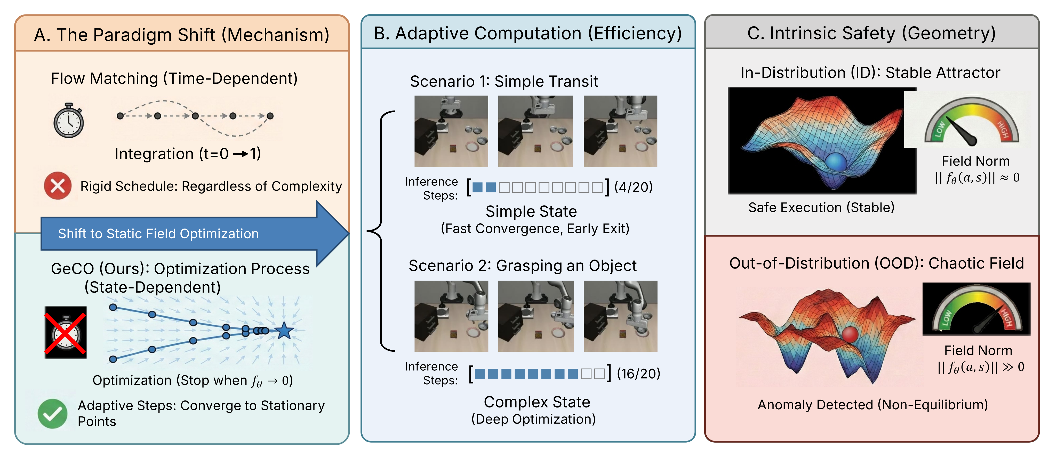
Generative policies such as Diffusion Policy and π₀ generate action chunks by iterative denoising. GeCO replaces explicit generative-time conditioning with a single field, so inference can stop according to its current residual rather than completing a prescribed noise-time path.
The intended benefits are state-dependent computation and a reused anomaly score without a separate detector network. The paper demonstrates these empirically; stationary fields need not be conservative energy gradients, and the training loss does not guarantee stable expert attractors or exclude low-residual OOD states.
2 Related Work
The work targets continuous diffusion/flow action heads, alongside VLM planning and video-based control. Flow matching supplies the regression framework, while noise-unconditional generation and equilibrium matching motivate a stationary formulation.
Energy-based control and implicit behavioral cloning are related, but this model directly predicts a vector field. Merely removing time input is insufficient: GeCO also rescales target velocity near demonstration endpoints.
3 Method
At each planning call, condition on camera images, proprioception and language; refine a short action chunk and execute a prefix before replanning. Training, stopping and anomaly scoring share the same learned field.
3.1 Revisiting Time-Conditioned Generative Control
A conventional velocity field depends on the partially denoised action, observation and generative time γ. Its integration traverses γ from 0 to 1. Different step counts or adaptive solvers are possible, but must still approximate that path.
GeCO removes this explicit time coordinate from the predictor. This changes the stopping criterion; it does not establish that every time-conditioned method must use a fixed evaluation budget.
Equations
3.2 Time-Unconditional Velocity Fields for Control
Mix an expert action a and Gaussian noise ε with γ sampled uniformly. Regress fθ on the scaled direction (ε−a)c(γ), without providing γ to the model. The inference update subtracts this direction, moving toward the expert endpoint.
The schedule satisfies c(1)=0. This makes the endpoint target vanish, but finite regression and averaging over hidden γ do not prove that all demonstrations become stable equilibria, that other equilibria are absent, or that the learned field is an exact potential gradient.
Equations 1–3
| (1) |
| (2) |
| (3) |
3.3 Optimization-Based Inference
Initialize from a prior such as Gaussian noise, repeatedly apply a←a−ηfθ(a,s), and stop at a small field norm or a maximum iteration count. Step sizes need not sum to one; their stability still matters.
Algorithm 1 retains the original twelve numbered lines. Its final assignment uses a⁽ᵏ⁾ after a loop updating a⁽ᵏ⁺¹⁾, leaving the exhaustion-case indexing ambiguous; the displayed pseudocode is unchanged. A small residual measures this field’s convergence, not physical task completion.
Equations 4–5
| (4) |
| (5) |
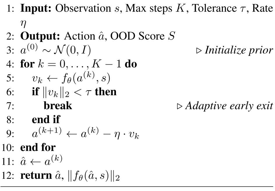
Selectable pseudocode
3.4 Intrinsic OOD Detection from Field Geometry
Use the norm at the final refined action as the planning-call anomaly score. Training should make familiar scenes easier to reach low-residual regions; the tested suite shift often produces larger residuals.
Reuse avoids a separate detector forward pass, though thresholds and filters require choices. OOD inputs can still produce low-residual fixed points; no calibrated epistemic uncertainty, universal separation or safety guarantee is proved.
Equations 6–7
| (6) |
| (7) |

Panel labels
3.5 Plug-and-Play Integration with VLA Systems
Keep the VLM conditioning pipeline and action interface of π₀-style systems, replacing the action head’s training objective and inference loop. Fix the existing time input at zero during fine-tuning. This reuses pretrained weights and architecture but is not an inference-only substitution without retraining.
Equation
4 Experiments
Experiments test small-policy efficiency, VLA transfer, suite-shift detection, hyperparameters and two physical tasks. These measure different outcomes; OOD discrimination is not equivalent to successful or safe control.
4.1 Policy Performance and Adaptive Computation
LIBERO tests compare diffusion, rectified flow and GeCO with the same action-generator family. The evaluation varies GeCO’s maximum refinement budget and records its actual average NFE.
The Efficiency-Performance Trade-off.
At a five-step cap, GeCO reaches 91.9% average success versus 90.0% for twenty-step rectified flow: 75% fewer field evaluations in this comparison. At a twenty-step cap, success reaches 93.5% with 11.6 average evaluations. A thirty-step cap yields 93.1%, so additional budget is not uniformly better. NFE reduction is not itself an end-to-end latency measurement.
Temporal Analysis: Computation Follows Complexity.
Figure 2 preserves six annotated rollout views. Spatial-task effort rises near pre-grasp alignment and placement; object-task effort can rise when selecting among candidates. These examples associate residual-driven effort with difficult phases, but do not isolate semantic reasoning or establish a causal complexity measure.
| Method | Max | Success Rate (%) | Efficiency | ||||
| Steps | Goal | Spat. | Obj. | Long | Avg. | NFE | |
| Diff. Policy | 100 (Fixed) | 82.9 | 91.4 | 88.9 | 82.7 | 86.5 | 100.0 |
| Rectified flow | 20 (Fixed) | 92.4 | 94.6 | 97.0 | 76.0 | 90.0 | 20.0 |
| GeCO (Ours) | 5 | 91.6 | 95.4 | 98.2 | 82.4 | 91.9 | 5.0 |
| GeCO (Ours) | 10 | 93.0 | 95.8 | 99.0 | 81.8 | 92.4 | 8.7 |
| GeCO (Ours) | 20 | 95.2 | 95.8 | 99.0 | 83.8 | 93.5 | 11.6 |
| GeCO (Ours) | 30 | 93.6 | 95.2 | 98.8 | 84.8 | 93.1 | 12.8 |
| Method |
Adjust Bottle |
Beat Block Hammer |
Blocks Ranking (Size) |
Click Alarmclock |
Click Bell |
Avg. | ||||||
| Easy | Hard | Easy | Hard | Easy | Hard | Easy | Hard | Easy | Hard | Easy | Hard | |
| ACT (Zhao et al., 2023) | 97.0 | 23.0 | 56.0 | 3.0 | 0.0 | 0.0 | 32.0 | 4.0 | 58.0 | 3.0 | 49.0 | 7.0 |
| (Black et al., 2024) | 90.0 | 56.0 | 43.0 | 21.0 | 7.0 | 1.0 | 63.0 | 11.0 | 44.0 | 3.0 | 49.0 | 18.0 |
| with GeCO | 86.0 | 66.0 | 52.0 | 36.0 | 0.0 | 0.0 | 72.0 | 16.0 | 42.0 | 21.0 | 50.0 | 28.0 |
4.2 Scalability to Vision-Language-Action Models
Fine-tune baseline and GeCO models from the same pretrained π₀-family weights for 30,000 steps. Holding the time channel at zero permits a stationary field without rebuilding the VLM. Benchmarks differ in batch size and input cameras, as detailed in Appendix C.
VLABench Result
On VLABench, π₀ with GeCO averages 36.0% versus 29.4% for π₀. Gains are largest on familiar manipulation and unseen textures; common-sense and semantic-instruction tracks improve, while cross-category transfer changes little. Aggregate gains coexist with individual-task regressions in Table 8.
RoboTwin 2.0 Benchmark Result
RoboTwin 2.0 evaluates five bimanual tasks in clean and randomized settings. π₀’s Hard average rises from 18% to 28%, while Easy changes from 49% to 50%. Hard gains include bottle adjustment, hammering and button/bell interaction; Blocks Ranking remains near zero. Some Easy tasks regress.
LIBERO Benchmark Result
Table 4 reports 93.9% for π₀+GeCO versus 94.2% for π₀, and 96.2% for π₀.₅+GeCO versus 96.9% for π₀.₅. The prose instead says 95.9% for the latter GeCO result; the table and original caption are retained. These results support approximate performance retention, not universal improvement.
| Method | Goal | Spat. | Obj. | Long | Avg. |
| + FAST (Pertsch et al., 2025) | 88.6 | 96.4 | 96.8 | 60.2 | 85.5 |
| (Black et al., 2024) | 95.8 | 96.8 | 98.8 | 85.2 | 94.2 |
| (Intelligence et al., 2025) | 98.0 | 98.8 | 98.2 | 92.4 | 96.9 |
| Ours () | 96.4 | 96.8 | 97.0 | 85.4 | 93.9 |
| Ours () | 96.4 | 97.4 | 98.6 | 92.4 | 96.2 |
4.3 Intrinsic OOD Detection from Optimization
The OOD experiment uses a residual from one planning call rather than an ensemble. It tests one controlled benchmark-suite shift, with separate planning-level discrimination and episode-level early stopping.
Experiment Setup.
Train on ten LIBERO-Goal tasks and test OOD detection on ten LIBERO-Spatial tasks. Similar objects appear in new layouts; this is a specific task/layout shift, not arbitrary sensor faults, unseen hazards or real-world OOD validation.
Baseline OOD Signal.
The comparison uses a Diff-DAgger-inspired training-loss proxy. Instead of estimating the original expectation with many samples, evaluate one Gaussian sample at fixed t=1 per planning call. Results therefore compare against this inexpensive proxy, not the full multi-sample detector.
Anomaly Score and AUROC Computation.
Use the last executed refinement’s field norm, with at most ten steps. Sample 500 ID and 500 OOD episodes and twenty planning calls per episode, yielding 10,000 instances per group. Equal calls per episode avoid giving long episodes extra weight; calls within an episode remain correlated.
Equations
Temporal Filtering and Early Reporting.
Filter residuals across refinement iterations within each planning call. The moving average uses five steps; the bucket accumulates positive excess above a threshold. Stop the whole episode on the first flagged call. Appendix D sets bucket leakage to zero, so its evaluated accumulator does not actually decay.
Equation
Quantitative Results.
Table 5 reports AUROC 0.93 for both GeCO filters versus 0.53 for the baseline, with 42.4%/44.3% reported interaction time saved. Its columns show TNR 82.4%/84.0% and TPR 89.7%/90.0%.
The text calls OOD positive, the caption defines TPR as ID specificity and TNR as OOD recall, and Appendix D targets 90% “TPR on ID.” These conventions conflict, so the column values are preserved without silently reinterpreting their labels. Threshold-selection data and treatment of unflagged episodes are not fully specified.
Equation
4.4 Ablations on Stationary Fields
In the DiT ablation, α=1 removes the target’s decay and gives 80.7% average success; tested α<1 choices give 90.9–92.2%, with α=0.8 best in this table. This supports velocity rescaling under the tested budget, not a convergence theorem. Appendix A specifies onset α₀=0.1, while this sweep emphasizes α=0.8; their relation to each reported configuration is not fully reconciled.
| Object | Goal | Spatial | Long | Avg | |
| 0.984 | 0.946 | 0.934 | 0.770 | 0.909 | |
| 0.968 | 0.954 | 0.958 | 0.802 | 0.921 | |
| 0.982 | 0.934 | 0.956 | 0.782 | 0.914 | |
| 0.982 | 0.942 | 0.956 | 0.778 | 0.915 | |
| 0.978 | 0.940 | 0.960 | 0.810 | 0.922 | |
| 0.932 | 0.840 | 0.898 | 0.558 | 0.807 |
4.5 Real-World Experiment
Physical tests deploy Galaxea G0 Plus and its GeCO variant on R1 Lite. Figures 3–4 retain the complete nut and chemistry-tube execution sequences.


Experimental Setup.
Both heads use the same teleoperated demonstrations and training-step budget. Tasks require nut/bolt alignment or insertion into a tube rack. The main text says ten independent trials per task, but Appendix E says twenty; the reported 25% baseline tube success is consistent with twenty binary trials.
Quantitative Results.
Nut success improves 30%→70%, mean NFE 10→5.06, and inference time 252.3→172.4 ms. Tube success improves 25%→80%, NFE 10→3.82, and time 254.6→150.3 ms. The reported latency reductions are 31.7% and 41.0%.
These are two small physical evaluations with randomized object poses. Better results at one data/training budget do not establish a sample-efficiency curve; demonstration counts, confidence intervals and hardware timing breakdowns are not supplied.
5 Discussion and Limitations
The authors leave rigorous performance, convergence-rate and OOD guarantees to future work. Practical limits include sensitivity to step sizes/thresholds, a narrow OOD split, small physical trials and incomplete protocol details. The low-norm criterion should remain an empirical control/detection heuristic.
6 Conclusion
A rescaled time-unconditional action field supports variable refinement effort and a reusable anomaly score. Results show useful efficiency–success trade-offs and compatibility with pretrained VLA heads, with benchmark-dependent gains. Stable-energy and safety interpretations remain hypotheses beyond the demonstrated experiments.
Impact Statement
The authors anticipate efficiency and operational-risk benefits and identify no harms beyond general automation concerns. The study does not provide a deployment safety case or broad hazard evaluation.
Appendix A Implementation Details for Adaptive Inference and Training
This appendix specifies the small-policy architecture, stationary-field schedule and receding-horizon sampler. These settings differ from the VLA and physical configurations below.
A.1 Codebase and Baselines
Implement GeCO on CleanDiffuser with the same backbone as continuous rectified flow. The comparison changes the field objective and sampling procedure.
A.2 Model Architecture
Use a one-dimensional diffusion transformer with frozen visual/language conditioning and cross-attention into the action sequence.
Vision-language condition.
Frozen DINOv2 and T5 encode two current RGB views and text. The conditioner uses embedding width 768, no history and frozen weights. The exact constructor/configuration names are retained below.
Equation
ViTAndT5VisionLanguageCondition
emb_dim=768
freeze=True
To=1
n_views=2
Policy backbone.
The action transformer uses sequence length 16, condition width 768, hidden width 384, six heads and twelve layers. Action dimensionality follows the environment. Baselines reuse these modules.
DiT1dWithACICrossAttention
x_dim=act_dim
x_seq_len=Ta(=16)
emb_dim=768
d_model=384
n_heads=6
depth=12
A.3 Adaptive Inference Setup
Apply up to thirty subtraction steps, stopping early by the residual norm. The step-size schedule is prescribed; only the number of executed steps adapts to the state.
Sampler.
The sampler repeatedly subtracts the predicted field times its step size. The source calls this gradient descent, although the network is not constrained to be an exact energy gradient.
Equation
Step-size schedule.
Use step sizes 0.1 for step 1, 0.05 for steps 2–4, 0.02 for steps 5–16 and 0.01 for steps 17–30. Stop below an L2 norm of 0.4.
Equations
A.4 Training Recipe and Hyperparameters
The training recipe combines frozen base encoders, a truncated linear velocity scale and sixteen-action prediction with eight-action execution.
Pretrained encoders.
Load google-t5/t5-base and facebook/dinov2-base. The source names the vision entry “ViT” in this configuration list.
Training details.
Equation (8) keeps c(γ)=λ until onset α₀, then decays linearly to zero at γ=1. The stated values are λ=4 and α₀=0.1. The later truncation sweeps use other α values; retain this stated recipe rather than replacing it with the best sweep value.
Equation 8
| (8) |
Constants.
Use observation horizon 1, action horizon 16, execute eight actions before replanning, and normalization parameters [0.5, 0.5, 0.5].
Appendix B Benchmarks
Three benchmarks test language-conditioned control under different task, appearance and coordination demands. The following protocols and complete per-task table accompany the aggregate results.
LIBERO.
LIBERO Goal varies goals, Spatial varies layouts, Object varies objects and Long tests composition. Each suite-specific policy trains for 30,000 steps and is evaluated over fifty rollouts. Inputs are two current RGB views and frozen T5 text; predict sixteen actions and execute eight.
RoboTwin 2.0.
RoboTwin 2.0 uses five tasks and 100 rollouts per Easy/Hard setting. Hard adds clutter, texture, lighting and tabletop-height changes while keeping task semantics. The official task success criteria determine the reported rates.
VLABench.
VLABench evaluates tracks 1, 2, 3, 4 and 6 with fifty rollouts under its standard protocol. Table 8 retains all ten primitive tasks, both methods and every track. Its fractions correspond to the percentages in Table 3; aggregate improvements do not hold for every individual task.
| Task | Track 1 | Track 2 | Track 3 | Track 4 | Track 6 | |||||
| Ours | Ours | Ours | Ours | Ours | ||||||
| add_condiment | 0.66 | 0.80 | 0.14 | 0.08 | 0.34 | 0.16 | 0.26 | 0.10 | 0.56 | 0.76 |
| insert_flower | 0.18 | 0.30 | 0.04 | 0.00 | 0.22 | 0.28 | 0.02 | 0.00 | 0.10 | 0.02 |
| select_book | 0.694 | 0.84 | 0.064 | 0.08 | 0.417 | 0.51 | 0.311 | 0.23 | 0.714 | 0.79 |
| select_chemistry_tube | 0.52 | 0.76 | 0.12 | 0.14 | 0.70 | 0.94 | 0.06 | 0.02 | 0.28 | 0.71 |
| select_drink | 0.52 | 0.78 | 0.224 | 0.30 | 0.08 | 0.10 | 0.10 | 0.04 | 0.44 | 0.66 |
| select_fruit | 0.38 | 0.56 | 0.46 | 0.52 | 0.083 | 0.14 | 0.06 | 0.18 | 0.30 | 0.32 |
| select_mahjong | 0.25 | 0.58 | 0.02 | 0.04 | 0.125 | 0.12 | 0.12 | 0.06 | 0.02 | 0.25 |
| select_painting | 0.46 | 0.22 | 0.26 | 0.12 | 0.50 | 0.60 | 0.56 | 0.76 | 0.30 | 0.18 |
| select_poker | 0.54 | 0.70 | 0.26 | 0.54 | 0.06 | 0.22 | 0.12 | 0.52 | 0.28 | 0.52 |
| select_toy | 0.50 | 0.52 | 0.36 | 0.34 | 0.38 | 0.32 | 0.12 | 0.10 | 0.18 | 0.28 |
| Avg_SR | 0.47 | 0.61 | 0.212 | 0.22 | 0.291 | 0.34 | 0.173 | 0.20 | 0.322 | 0.45 |
Appendix C VLA Training Details.
Fine-tune π₀/π₀.₅ in OpenPI from their base checkpoints on LeRobot-format data, using 30,000 gradient steps throughout.
RoboTwin 2.0.
For RoboTwin, train a separate π₀ per task with batch size 32. Inputs are cam_high, cam_left_wrist, cam_right_wrist and observation.state.
LIBERO.
For LIBERO π₀, use physical-intelligence/libero data and the pi0_base checkpoint, batch size 32. π₀.₅ uses batch size 256, AdamW, gradient clipping 1.0, EMA decay 0.999 and cosine learning rate with 10,000 warmup steps and peak 5×10⁻⁵.
VLABench.
VLABench uses vlabench/vlabench_primitive_ft_lerobot, batch size 256 and 30,000 steps.
Appendix D OOD Detection Settings
The full OOD protocol specifies sampling, filters and a fixed episode horizon. Some operating-point definitions remain inconsistent with the main text and Table 5.
ID/OOD split.
Train one policy on the ten LIBERO-Goal tasks; designate the ten LIBERO-Spatial tasks as OOD. This evaluates a suite/layout shift within one simulator.
Episode and planning-call sampling.
Collect 500 episodes from each suite and randomly select J=20 planning calls per episode. Each selected call is an AUROC instance, rather than each complete episode.
GeCO score (optimization-dynamics signal).
Record per-refinement L2 norms for at most ten steps. The raw planning score is the final executed norm, including early-stopped calls.
Equation
Temporal filters and triggering rule.
Within a call, use a five-step moving average or positive-excess bucket. Fix (τma,τ,λ,B)=(0.6,0.5,0,0.7) for the experiments. Zero leakage makes the bucket a non-decaying excess accumulator; handling the moving average before five available samples is not stated.
Equation
Baseline score (training-loss proxy).
Construct a noisy generated action with one Gaussian draw and evaluate the flow-matching regression loss. The main text fixes t=1; the appendix writes an expectation but describes a single-sample proxy. It mentions a total diffusion-step count T without using it in the displayed interpolation.
Equations
AUROC computation.
Sweep score thresholds over 10,000 ID and 10,000 OOD planning instances. Here the source explicitly labels OOD positive and ID negative.
Operating point (TNR/TPR).
Select a threshold near 90% “TPR on ID instances,” then report TNR. This conflicts with the preceding OOD-positive convention; Table 5’s caption also swaps the conventional names. No held-out threshold-calibration split is specified.
Early reporting and Time Saved.
Terminate an episode at its first detection. Compute 1−treport/300 and average over OOD episodes. This measures avoided environment steps against the fixed 300-step horizon, not measured wall-clock savings; the treatment of episodes with no detection is unspecified.
Equation
Appendix E Real World Experiment Settings
Physical deployment uses Galaxea R1 Lite and G0 Plus, with object-pose variation in two precision-manipulation tasks.
Hardware Configuration.
Inputs are a head camera, two wrist cameras and joint/gripper state. The physical control frequency is 15 Hz and the execution action chunk has sixteen actions. Reported inference times exceed one 15-Hz control interval, so chunk execution and inference latency should not be conflated.
Data Collection and Task Description.
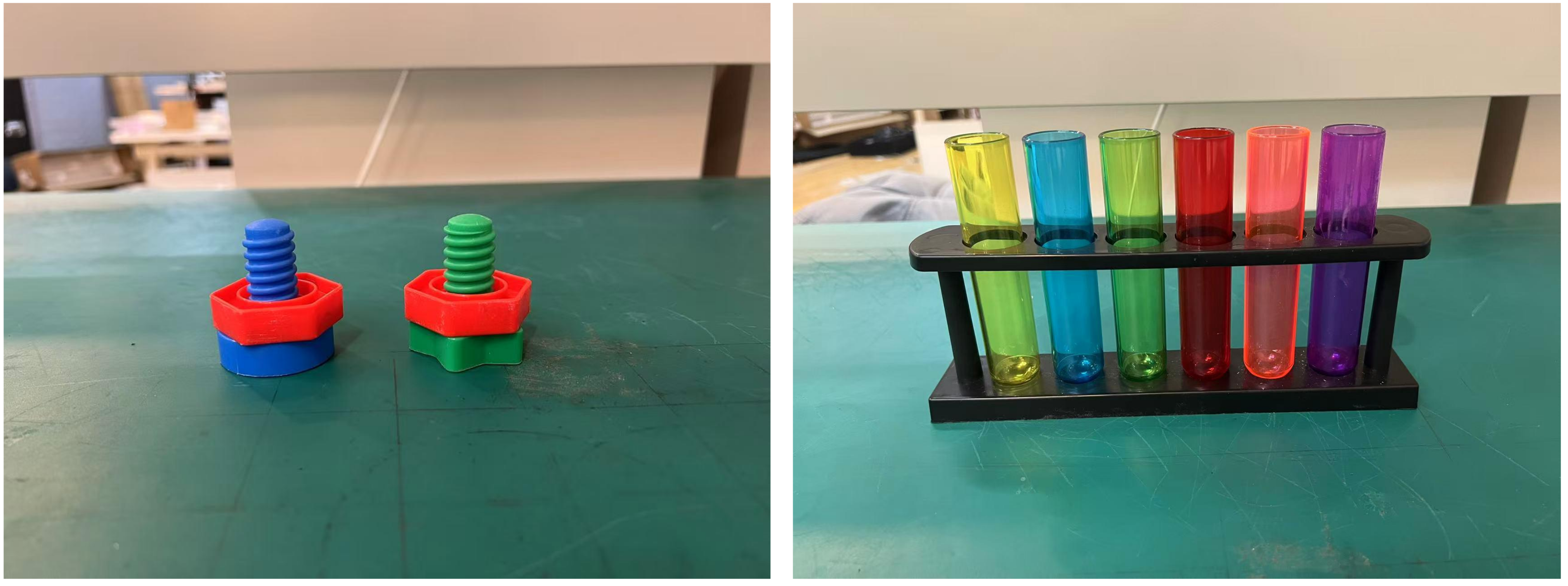
Nut success requires both plastic nuts fully threaded onto their respective bolts. Tube success requires grasping from a randomized pose and fully seating the tube in the correct tight-tolerance rack slot without dropping or tipping it. Rack position and rotation also vary; Figure 5 preserves both setups.
Training Details.
Initialize from pretrained G0 Plus, fix time conditioning to zero, and fine-tune for four full epochs with batch size 32. Use AdamW, peak learning rate 2.5×10⁻⁵, cosine decay and 200 warmup steps. The demonstration count is not given.
GeCO Inference Setup.
Cap refinement at ten steps; decay step size from 0.25 to 0.02 and stop below norm 1.5. The complete intermediate schedule is not tabulated. Reaching the cap allocates more computation but does not guarantee successful alignment.
Equation
Evaluation Protocol.
This appendix reports twenty independent trials per task and method, unlike ten in the main text. Randomize nuts, bolts, tubes and racks. The baseline always uses ten field evaluations; GeCO’s count varies. Success and average NFE are reported without uncertainty intervals.
Appendix F Detailed Analysis of Real-World Adaptive Computation
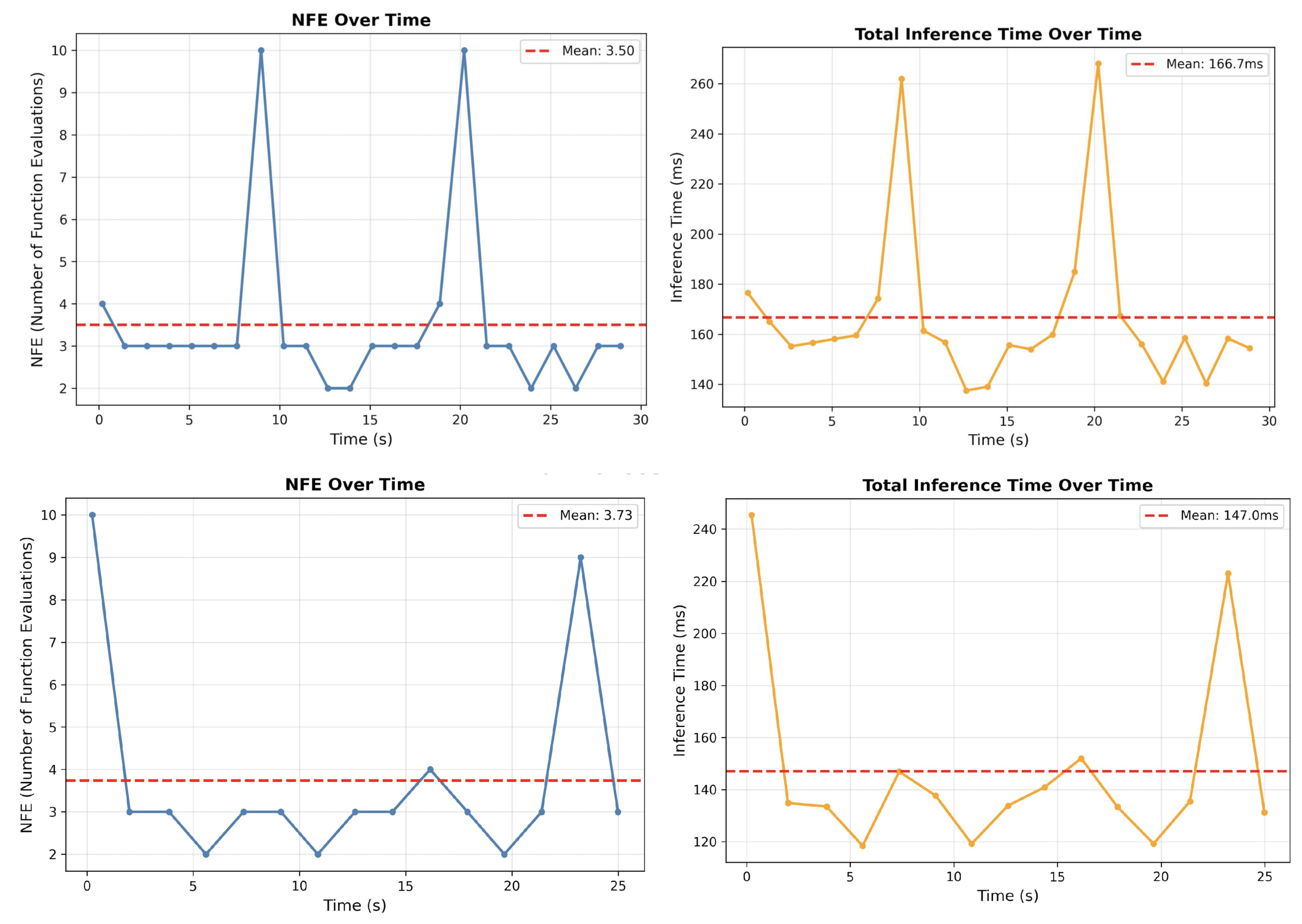
Figure 6 retains all four plots of NFE and inference latency from representative physical rollouts. Nut means are 3.50 evaluations and 166.7 ms; tube means are 3.73 and 147.0 ms. These single-rollout summaries differ from the aggregate means in Table 7.
Peaks reach nine or ten evaluations near demanding phases, while easier motion uses two or three. Latency broadly follows NFE, supporting adaptive computation in these examples rather than proving a universal complexity estimator.
Appendix G Additional Ablation Studies
Additional sweeps test VLA truncation, the stopping threshold and fixed step-size alternatives. They show where the reported formulation is robust and where configuration still matters.
G.1 Ablation Study: Effect of Truncation Parameter α
The VLA sweep gives 81.0%, 96.2% and 92.2% average LIBERO success for α=0.6, 0.8 and 0.9. The smaller setting particularly hurts Long. The authors attribute this to smoothness/stiffness, but do not measure Lipschitz constants or prove the proposed mechanism. The text’s Table 6 cross-reference refers to the earlier DiT sweep; these results are Table 9.
| Success Rate (%) | |||||
| Goal | Spat. | Obj. | Long | Avg. | |
| 85.8 | 98.0 | 91.6 | 48.6 | 81.0 | |
| 96.4 | 97.4 | 98.6 | 92.4 | 96.2 | |
| 95.8 | 97.8 | 94.0 | 81.2 | 92.2 | |
G.2 Ablation Study: Effect of the Early-Stop Threshold τ
Tightening the stop threshold to 0.4 gives 93.5% success at 11.6 average steps. Thresholds 0.6 and 0.8 give 92.35%/7.7 steps and 91.9%/6.6 steps. A stricter residual threshold improves this trade-off but does not establish convergence to an exact expert equilibrium.
| LIBERO Object | LIBERO Goal | LIBERO Spatial | LIBERO Long | Avg | Avg. Steps | |
| 99.0 | 95.2 | 95.8 | 83.8 | 93.5 | 11.6 | |
| 98.8 | 94.0 | 95.6 | 81.0 | 92.35 | 7.7 | |
| 96.8 | 93.2 | 96.0 | 81.6 | 91.9 | 6.6 |
G.3 Ablation Study: Robustness to Fixed Step-Size Schedules
Twenty fixed steps of size 0.02 reach 93.05% from the four printed suite rates, rounded to 93.1% in Table 11, versus 93.5% for the current schedule. Other fixed choices range 90.3–92.0%. The schedule is not uniquely necessary, but these comparisons alone do not isolate stationary-field learning from every other implementation choice.
| Step-size schedule | LIBERO Object | LIBERO Goal | LIBERO Spatial | LIBERO Long | Avg |
| 97.0 | 92.0 | 94.8 | 77.2 | 90.3 | |
| 98.0 | 94.8 | 95.4 | 84.0 | 93.1 | |
| 98.4 | 95.0 | 94.2 | 80.4 | 92.0 | |
| 98.0 | 95.0 | 95.0 | 77.4 | 91.4 | |
| Current schedule | 99.0 | 95.2 | 95.8 | 83.8 | 93.5 |