Overview
This edition covers arXiv v 2 dated 20 October 2026, accepted at CoRL 2026. The nine authors are affiliated with Disney Research and NVIDIA in Zurich; Vassilios Tsounis, Guirec Maloisel and Christian Schumacher share first authorship. Kamino project.
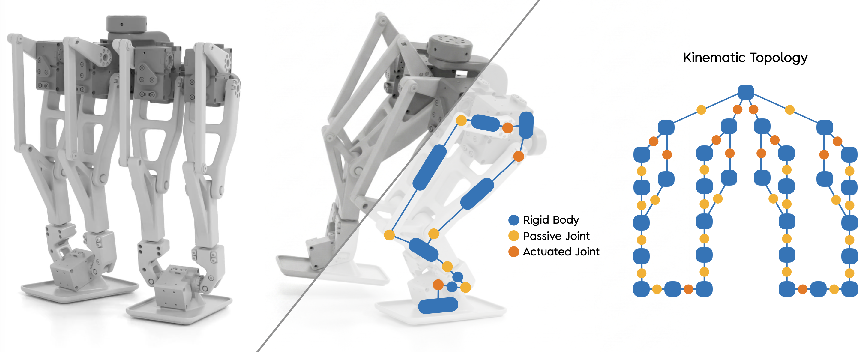
At a glance
Kamino simulates rigid-body mechanisms with closed kinematic loops on a GPU. Every body has an independent pose; a globally coupled proximal ADMM solver resolves joint constraints, limits and frictional contacts. The Newton/Warp implementation also batches worlds with different robot morphologies.
The demonstrations include a six-loop biped trained in 4,096 environments. The main benefit is robust constraint/contact handling for mechanically complex robots; the paper also reports substantially lower throughput than MJWarp on a simple tree-structured model.
1 Introduction
Minimal coordinates make tree-structured robots efficient, but loops require additional closure constraints and a choice of articulation tree. Ill-conditioned, tightly coupled loops and contacts can challenge local iterative solvers or compliant contact approximations.
Kamino builds on prior quaternion-based constrained dynamics and rigid multi-body solver analysis, using proximal contact methods. Its contribution is a GPU implementation and learning integration: maximal coordinates, hard-contact complementarity, dense or matrix-free global solves, and heterogeneous worlds. The broad first-of-its-kind claim is the authors’ positioning, not an exhaustive independent priority assessment.
Newton supplies assets/collisions and Warp compiles Python kernels to CUDA. This reduces the need to replace a real looped mechanism with a tree approximation, while retaining numerical tolerances, stabilization and finite-step integration.
2 Method
The method combines a Newton-compatible simulation/reset interface, a reaction-space formulation of maximal-coordinate dynamics, and a proximal ADMM solver. The appendices retain the full mechanics, implementation and algorithm.
2.1 High-level API
SolverKamino implements Newton’s SolverBase. Static Model data and dynamic State, Control and Contacts live on the GPU. step reads the current state and controls, solves dynamics, integrates and writes a second state buffer; swapping buffers supports CUDA graph replay. Contacts come from Newton or Kamino’s internal detector.
reset accepts joint coordinates, actuated DoFs, base states or complete body states, optionally masked by world. Its loop-aware forward-kinematics solver constructs consistent body poses; arbitrary joint assignments need not themselves satisfy closed-loop geometry. Config groups integration, stabilization and tolerance choices. Both exact API calls are retained.
solver.step(state_in, state_out, control, contacts, dt)
solver.reset(state, world_mask, …)
2.2 Constrained Dynamics in Maximal Coordinates
Each body has an SE(3) pose and six-dimensional twist. A block-diagonal mass matrix couples to joint, limit and contact reactions through the Jacobian. Implicit PD gains, armature and viscous damping enter the constraint system rather than a separate explicit force update.
Eliminating body velocities yields a Delassus reaction-space problem. The de Saxcé correction adds a slip-dependent normal velocity term so Coulomb sliding obeys maximum dissipation without artificial separation. Eq. (1) retains the paper’s nonlinear optimization statement; the implemented iteration freezes this correction at the previous iterate.
Heterogeneous worlds use a two-dimensional kernel grid indexed by world and maximum problem dimension. Threads outside a world’s actual dimension exit by mask. This permits varied topology but can leave padded work and imbalance.
Equations 1
| (1) |
2.3 Proximal-ADMM Solver
PADMM alternates a global linear solve, projection onto admissible reaction cones, and a dual update. The global solve dominates cost. Small problems use a dense Delassus matrix and block-Cholesky factorization; larger problems use a block-sparse Jacobian and matrix-free Conjugate Residual iterations. Sparse Jacobian storage can also feed the dense factorization path.
3 Experimental Results
Comparisons cover Newton’s Kamino, MJWarp and XPBD, plus CPU MuJoCo. GPU solvers use 32-bit arithmetic; CPU MuJoCo uses its default 64-bit precision. Models include simple analytic systems, manipulation, looped robots and heterogeneous Ant variants. These implementation and precision choices are part of the comparison.

3.1 Physics Validation
Validation separates analytic single-phenomenon tests, a manipulation demonstration and residual measurements on full robot models. Physical agreement and computational speed are evaluated separately.
Elementary Examples
A sliding box, bouncing ball, unequal-mass box stack and passive four-bar linkage isolate friction, restitution, mass-ratio conditioning and loop closure. Kamino closely follows analytic references; the linkage still requires choosing a Baumgarte weight to trade constraint drift against energy behavior.
MJWarp’s compliant formulation and XPBD’s local position-level iterations exhibit different errors in these chosen tests. Results depend on the stated settings; they do not establish uniform superiority for every contact model, task or tuning budget.
Manipulation
A two-finger arm stacks cubes using inverse kinematics, PD position targets and feedforward gravity compensation. All 100 runs with randomized initial conditions succeed. This is a simulation stability demonstration, not a controlled manipulation comparison or measured real-robot success rate.
Physical Accuracy on Robotic Systems
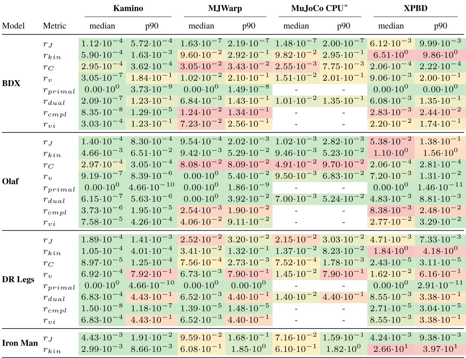
Table 1 measures accumulated joint/contact configuration error on independent trajectories and per-step velocity/complementarity error on common states sampled from a 10 kHz Kamino trajectory. Median and 90 th-percentile summaries deliberately reduce the influence of hard impact frames; no continuous collision detection is used.
Kamino uses 200 PADMM iterations; XPBD uses 20, increased to 200 for Iron Man to avoid divergence. Contact forces are unavailable for CPU MuJoCo, leaving three residuals unreported. BDX, Olaf and DR Legs fall under random torques; Iron Man is unactuated with collisions disabled.
Kamino is strong on many velocity and complementarity residuals, especially on looped systems, but does not win every cell. Tree-based MuJoCo nearly eliminates BDX joint-position error; XPBD has smaller penetration in several rows, and some 90 th-percentile velocity residuals favor another solver. The full values and original color shading remain available.
* We do not measure for MuJoCo CPU as contact forces are unavailable.
3.2 Simulation Throughput
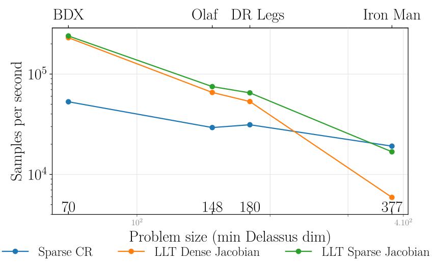
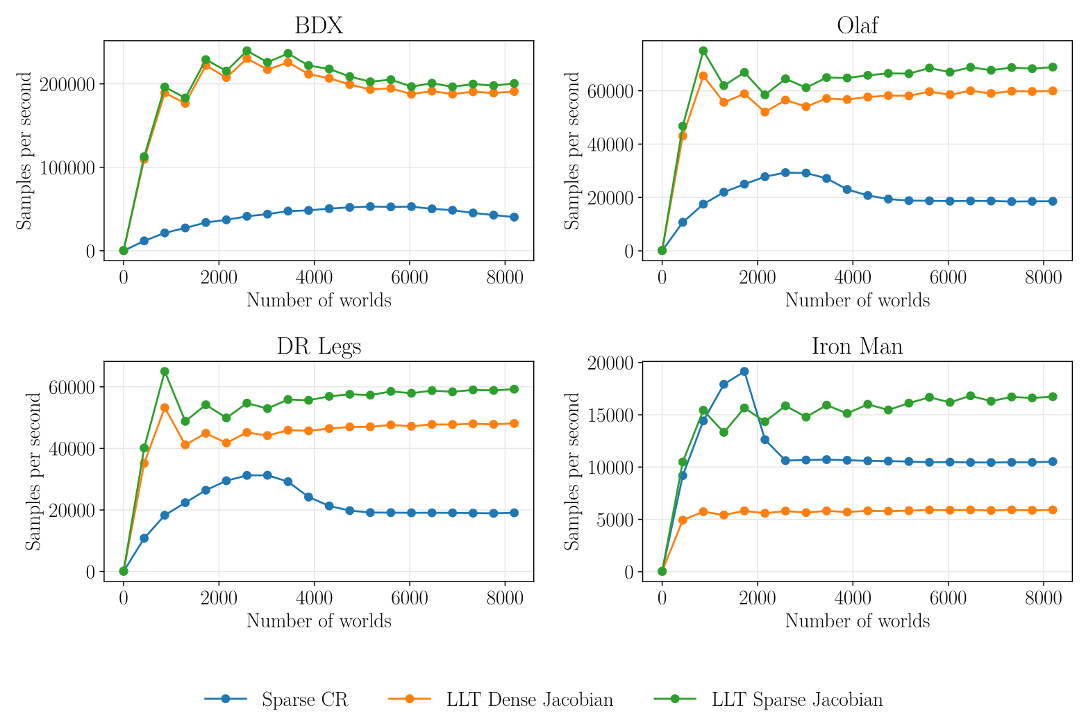
The best linear solver changes with problem size: sparse-Jacobian LLT performs well on smaller systems; matrix-free CR helps large systems such as Iron Man. Sparse-Jacobian LLT consistently beats its dense-Jacobian variant in the reported throughput tests.
On BDX, Kamino reaches 240,000 samples/s, versus 580,000 for XPBD and 6.1 million for MJWarp: about 2.4× and 25.4× slower, respectively. These are batched simulator steps per second, not equal-error or equal-simulated-time comparisons.
3.3 Simulation of Complex Mechanisms
Three controlled animation/stress scenarios test sensitivity to topology, mass ratios and loop count. Different solvers receive different time steps or tuning where needed for stability.
DR Legs
With identical gait commands, MJWarp’s pelvis-rooted articulation walks while its left-foot-rooted tree falls. Kamino walks at 1.25 ms steps. XPBD needs 0.2 ms steps and half-speed animation in this demonstration. The maximal-coordinate representation avoids choosing an articulation root.
Iron Man
Iron Man combines 13 loops with large link-mass ratios. Kamino follows the animation at 5 ms; MJWarp requires tuned closure parameters and 0.2 ms, while XPBD uses 100 iterations and 0.2 ms to avoid excessive actuator compliance. Contacts are disabled.
Hoberman Sphere
A spinning Hoberman sphere expands and contracts in zero gravity with contacts disabled. All solvers handle the stated initial condition at 2 ms. Larger angular velocity or external loading increases MJWarp’s closure-tuning demands; this is a numerical stress test, not validation of physical sphere dynamics.
3.4 Reinforcement Learning
Policies are trained for BDX, Olaf, DR Legs and three Ant morphologies. Unlike the earlier Olaf controller, which separated looped shoulders/jaw into PD control, Kamino supports one learned policy for the full system.
Across ten DR Legs training seeds, the paper reports 98.5±0.4% episode survival and under 2% reward variation. The meaning of the ± statistic is not specified. BDX and Olaf transfer to physical hardware in the supplementary video; DR Legs and heterogeneous Ant results here are simulation demonstrations.
4 Limitations
Repeated global solves make Kamino slower than MJWarp/XPBD on current benchmarks. Hybrid maximal/minimal-coordinate formulations and further implementation work may reduce this cost. Only linear 3 D Coulomb friction is supported: torsional/rolling contact friction and joint static friction are absent.
Real-world evaluation is limited to BDX and Olaf demonstrations. Hard contact is a model choice, not an absence of numerical approximation: finite steps, single precision, solver tolerances, warm starts and constraint stabilization still matter.
5 Conclusion
The paper establishes a practical GPU path for rigid robots whose mechanics include nested loops and heterogeneous morphology. Its evidence supports a useful accuracy/robustness trade-off, with throughput and limited real-world validation remaining constraints. Flexible bodies, cables, transmissions and granular media are proposed extensions rather than demonstrated capabilities.
Acknowledgments
The authors acknowledge Disney Research colleagues, NVIDIA’s Newton collaborators and reviewers, and Google DeepMind researchers for contributions, code review and technical discussions.
Appendix A Appendix
The appendix supplies the full dynamics and residual definitions, PADMM implementation, structural model counts, analytic validation, throughput/memory measurements and complete learning-task specifications.
A.1 Constrained Rigid Multi-Body Dynamics in Maximal Coordinates
Every body stores position, unit-quaternion orientation and world-frame linear/angular velocity. Its 6×6 mass block contains scalar translational mass and rotated inertia. The global mass matrix is block diagonal; joint, limit and contact Jacobian rows encode the coupling. All defining equations and dimensions are retained.
Equations 2–4
| (2) |
| (3) |
| (4) |
A.1.1 Signorini-Coulomb & Bipotential Contact Model
Normal velocity and nonnegative normal reaction obey Signorini complementarity. Tangential reaction lies in a friction disk and opposes slip at maximum dissipation. The de Saxcé bipotential construction offsets normal velocity by friction coefficient times tangential speed before testing dual-cone complementarity.
The combined reaction set is unrestricted for bilateral joints, nonnegative for limits and a product of Coulomb cones for contacts. The exact cone inclusion remains below; this is a non-associated friction law rather than an ordinary uncorrected cone projection on raw velocity.
Equations 5–7
| (5) |
| (6) |
| (7) |
A.1.2 Discrete-Time KKT Formulation and Dual Transcription
Semi-implicit Euler, or an optional Moreau–Jean midpoint scheme, gives the block KKT system. Eliminating post-step body velocity produces D = JM⁻¹Jᵀ + R and a free velocity that includes external forces and stabilization/restitution targets. R represents implicit joint dynamics, not generic contact softening.
The paper calls the resulting expression an NSOCP and cites a prior equivalence proof sketch. Since the correction depends on the unknown velocity, the frozen-correction PADMM iteration should be distinguished from directly minimizing a fixed convex quadratic; no new global convergence guarantee is proved here.
Equations 8–13
| (8) |
| (9) |
| (10) |
| (11) | ||||
| (12) | ||||
| (13) |
A.1.3 Joint-Space Dynamics
Implicitly discretize a joint’s armature, viscous damping, feedforward torque and PD feedback. The effective diagonal joint inertia combines a, Δtb, ΔtKd and Δt²Kp. Eliminating joint velocity through its body Jacobian adds the resulting constraint to the same KKT system. Equations (14)–(19) retain every sign and term.
Equations 14–19
| (14) |
| (15) |
| (16) |
| (17) |
| (18) |
| (19) |
A.1.4 Physics Metrics
The metrics distinguish configuration violations, joint-velocity error, inward contact velocity, primal cone feasibility, dual-cone feasibility, complementarity and natural-map distance. Infinity norms capture the worst constraint within each sampled state; median/p 90 aggregation then summarizes states.
The natural-map residual combines feasibility/complementarity at a fixed state, while position errors capture accumulation. These quantities have different units/scales and are not interchangeable accuracy scores. Joint reaction residuals are omitted from the cross-solver comparison because most solvers do not expose those forces.
Equations 20–26
| (20) |
| (21) |
| (22) |
| (23) |
| (24) |
| (25) |
| (26) |
A.2 PADMM Solver Details
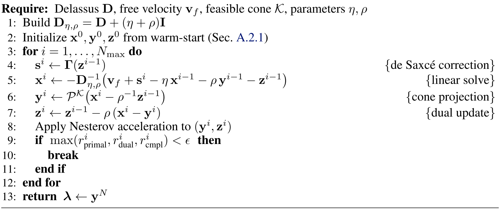
The algorithm separates unconstrained reaction x, feasible reaction y and a velocity-like dual variable z. Freeze the de Saxcé estimate, solve the shifted Delassus system, project and update the dual. The expensive factorization/operator setup is reused within a step while active constraints and solver parameters remain fixed.
The proximal η and augmented-Lagrangian ρ shift the numerical solve; they should not be confused with changing the physical contact law. The complete 13-step pseudocode and its input line remain, including warm starts, acceleration and residual stopping.
Selectable pseudocode
Equation
A.2.1 Practical GPU Implementation
Four engineering choices reduce iteration cost or improve convergence: restarted momentum, temporal warm starts, diagonal scaling and captured GPU loops.
Nesterov Acceleration
Nesterov extrapolation accelerates consensus and dual variables. The momentum coefficient follows the preserved recurrence; when the combined residual stops decreasing, acceleration resets to one to limit oscillation, following adaptive restart.
Equation
Warm-starting
Cache converged reactions between steps. For changing contacts, associate cached values using geometry pairs and nearest contact positions. This is a practical correspondence heuristic, not an invariant guarantee when contact topology changes.
Diagonal Preconditioning
Compute Jacobi scaling from the Delassus diagonal once per step and solve the scaled shifted system. This improves conditioning in the single-precision implementation. The exact preconditioner and operator remain below.
Equation
Graph Capture
Warp’s wp.capture_while captures the iterative solver as a CUDA graph with conditional replay. Fixed array shapes permit replay each time step; a per-world mask stops work for converged worlds. Operator constancy applies within a step, not across changing configurations.
A.2.2 Linear System Solve
Dense LLT factors the shifted matrix once per step and reuses triangular solves. The sparse path stores at most two six-coefficient body blocks per scalar constraint row and applies JM⁻¹Jᵀ plus R and the diagonal shift without forming D.
Matrix-free CR is warm-started from the previous PADMM iterate; the experiments use as few as 15 inner iterations. Pre-baking the inverse mass and diagonal scaling into Jacobian data avoids repeated passes. Adaptive ρ is cheaper here because dense LLT would need refactorization. The small inner budget is an empirical choice, not an accuracy guarantee for arbitrary conditioning.
Equation 27
| (27) |
A.3 Simulation Models Overview
Table A.1 records every model’s bodies, actuated/passive joints and independent loops. DR Legs has 31 bodies, 12 actuators, 24 passive joints and six loops; Olaf has three loops; Iron Man has 67 bodies and 13 loops; Hoberman has 240 bodies and 182 loops.
BDX and the three Ant variants are trees. The manipulation model is a seven-axis Panda with a two-finger Franka Hand. These systems exercise different topology and contact regimes rather than a uniform task distribution.
A.4 Elementary Examples
Four elementary tests compare trajectories or constraints against first-principles references. The complete plots retain all solver variants, iteration settings and analytic curves.
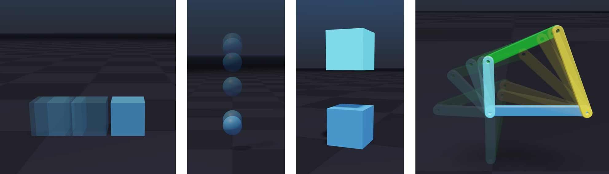
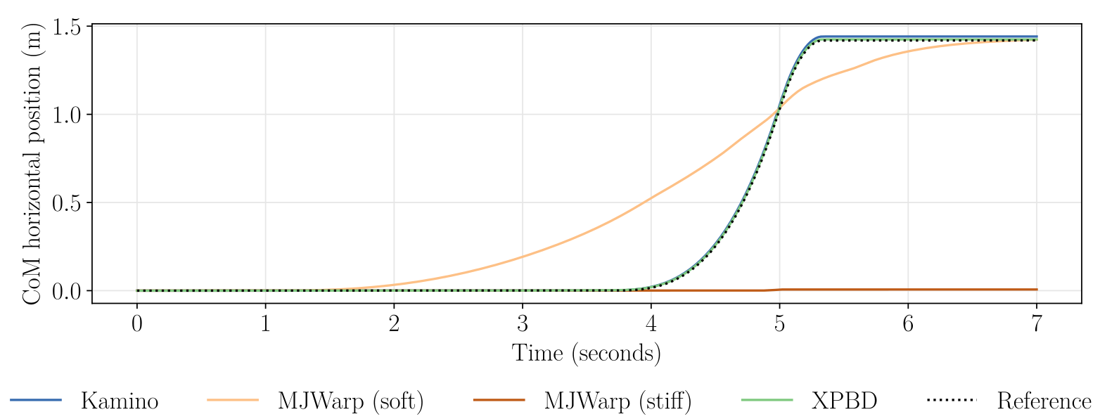
Box on Plane
Ramp horizontal force from zero to 1.5 times the stick-slip threshold, remove it and let friction stop the box. The reference integrates analytic forces at 0.1 ms. Kamino matches the trajectory; XPBD needs 20 rather than two iterations and still permits slow premature sliding.
MJWarp’s stiff default over-sticks. Softer tuning can match final distance while distorting the trajectory and causing penetration/wobble. Equal corner loads at rest are observed for all solvers; the reported minimum-norm behavior is demonstrated in this example, not a proof for every warm start or contact geometry.
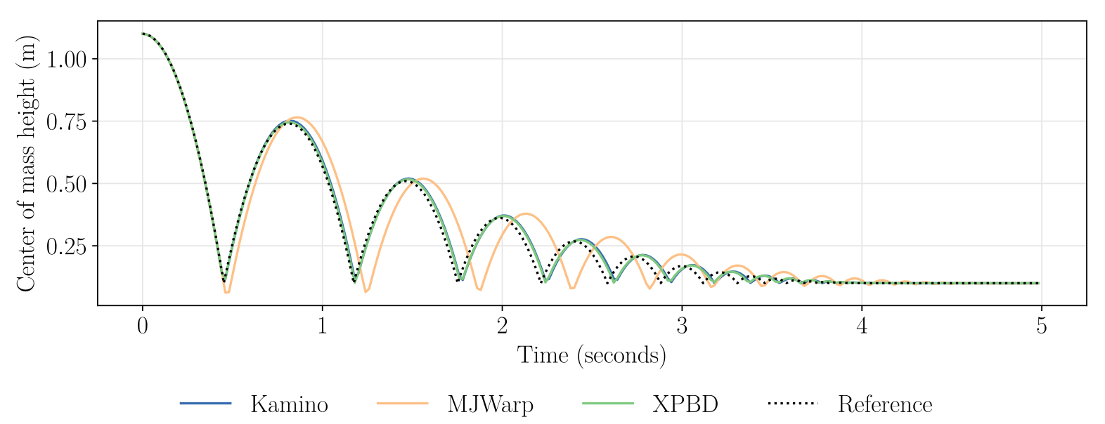
Bouncing Ball
Drop a ball with restitution 0.8 and compare repeated parabolic flights. Kamino and XPBD closely match the analytic trajectory. MJWarp approximates restitution through an underdamped spring–damper contact, coupling bounce behavior to compliance and allowing visible penetration.
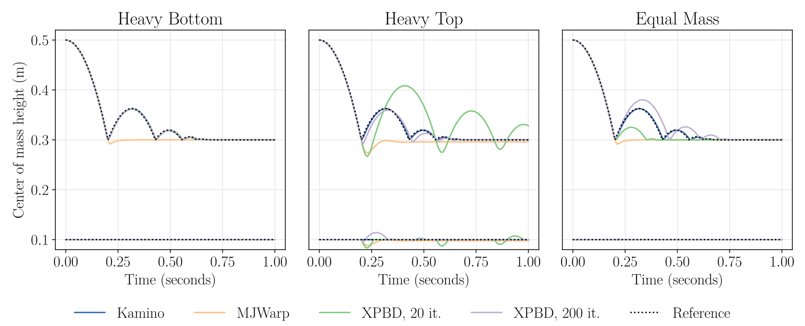
Stacked Boxes
Drop one box onto another with masses 100:1, 1:100 and 1:1. The analytic trajectory is mass-independent. Kamino remains close across ratios; softened MJWarp penetrates more under a heavy top box, and this test does not tune MJWarp to reproduce restitution.
XPBD’s local iteration is sensitive to mass order; even 200 iterations leave visible error in the difficult case. The plots preserve both its 20- and 200-iteration variants.
Four-Bar Linkage
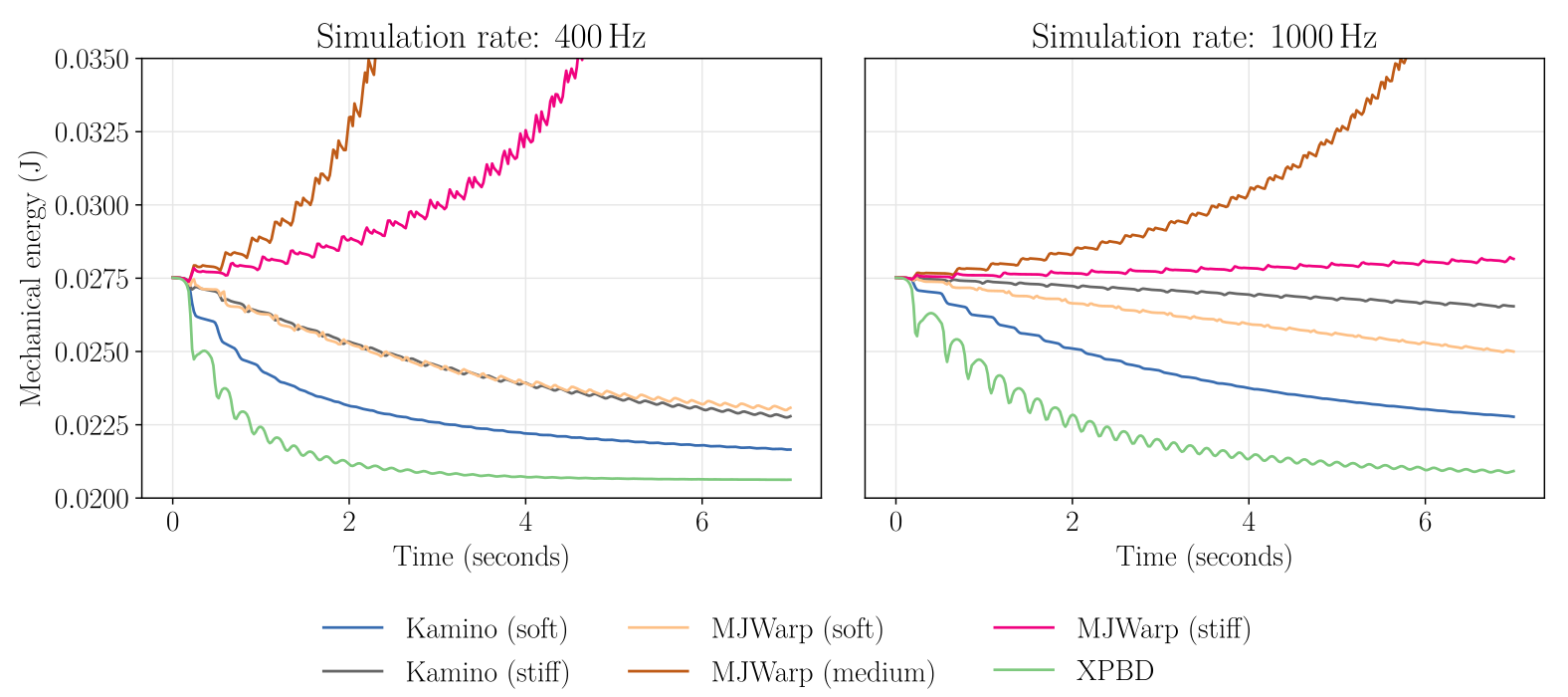
A passive four-bar linkage should conserve mechanical energy. Compare 400 and 1,000 Hz, Kamino stabilization weights 0.01/0.1, MJWarp time constants 0.1/0.01/0.001 and zero-compliance XPBD. Stronger stabilization trades energy behavior against geometric drift.
At 1,000 Hz, Kamino’s stiff maximum residual is 3.6×10⁻⁴, versus 1.0×10⁻⁴ for stiff MJWarp and 2.2×10⁻⁴ for XPBD; at 400 Hz XPBD reaches 1.4×10⁻³ but dissipates most strongly. MJWarp can inject energy nonmonotonically with stiffness. Kamino is reasonably dissipative with a monotonic stabilization trend, not exactly energy-conserving.
| Sim. rate | Kamino | MJWarp | XPBD | |||
|---|---|---|---|---|---|---|
| Soft | Stiff | Soft | Medium | Stiff | ||
A.5 Performance
Additional benchmarks separate batched throughput from memory use across solver representations and hardware. Model dimension is reported without active contacts/limits even though measured trajectories include them.
Throughput
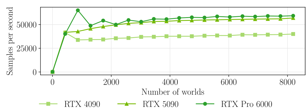
Random actuator torques are held for 0.5 s on BDX/Olaf/DR Legs, yielding falls, contacts and joint limits; Iron Man passively collapses without actuation. Disable early stopping and fix 100 PADMM/15 CR iterations to reduce convergence-dependent timing variation.
Throughput saturates after a few thousand worlds. Sparse CR can decline at larger batches; dense curves show GPU execution-wave tail effects. RTX 4090/5090/Pro 6000 measurements provide hardware-specific comparisons, not universal speedups or equal-tolerance solver rankings.
Memory Usage
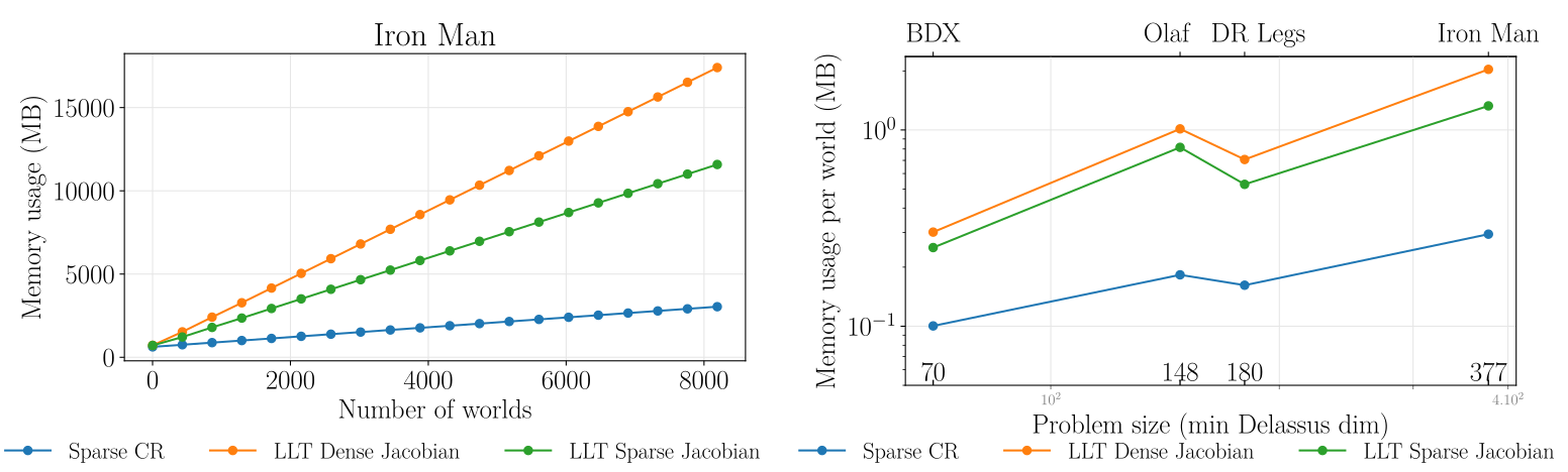
All memory is allocated when creating the model/solver, so there is no separate dynamic peak during graph replay. Homogeneous-batch memory grows approximately linearly with world count plus shared geometry overhead. Sparse representations scale better per world, although memory is not the limiting factor for these tested systems.
A.6 Complex Simulation Examples
The following details distinguish the predefined-animation experiments from RL training and specify the disabled-contact stress tests.
DR Legs
Gait setpoints are sampled at 100 Hz and interpolated for implicit PD control. MJWarp’s articulation trees come from breadth-first search rooted at pelvis or left foot, with actuated joints required in the tree and passive joints used for loop closures. This construction explains the topology-choice comparison.
Iron Man
Iron Man tracks a 100 Hz animation with contacts disabled. Its 13 loops route indirect actuation from the base/torso, and moving masses range 0.012–49.20 kg. Tuned MJWarp and 100-iteration XPBD require 0.2 ms steps in the reported stable configuration; Kamino uses 5 ms.
Hoberman Sphere
Initialize the passive sphere at 0.5 rad/s in zero gravity with no collisions. Expansion and contraction alternate through its linkage geometry and momentum. At this speed all solvers have reasonably close constraint violations; stronger excitation stresses MJWarp’s closure settings.
A.7 Reinforcement Learning
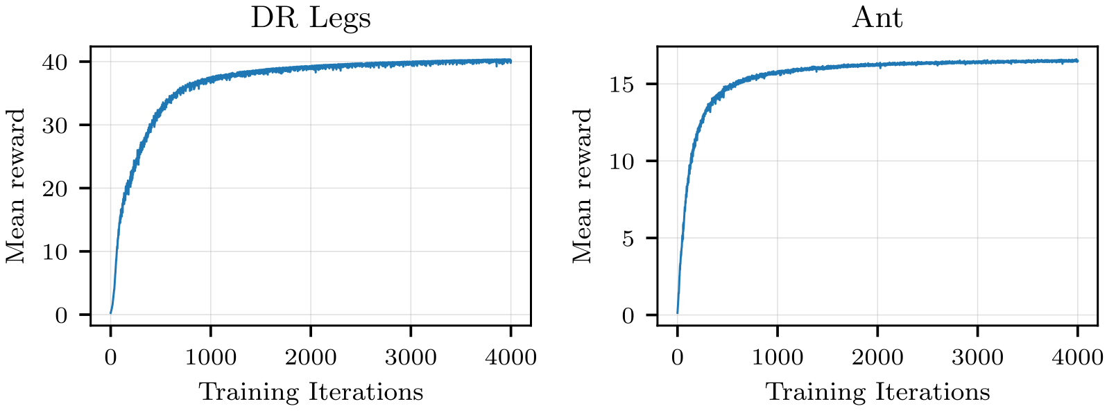
DR Legs and heterogeneous Ant use PPO, three 512-unit ELU hidden layers and 4,096 worlds. The simulator runs at 4 ms with decimation 5, giving 50 Hz position-target policies. Four thousand iterations take about 3.5 h for DR Legs and 2.8 h for Ant on an RTX 5090.
The displayed learning curves show the task rewards. The paper does not provide a full PPO hyperparameter table or a matched training-time benchmark against other simulators; BDX/Olaf reuse earlier learning setups.
A.7.1 DR Legs
Track planar linear and yaw commands for 10 s episodes, sampled within±0.3 m/s and±0.8 rad/s. A one-second gait period approximates a pendulum at the nominal 0.265 m standing height. This prescribed phase and foot shaping help structure the learned gait.
Action Space
Twelve normalized actions in[−1,1] specify targets for the actuated joints, tracked by implicit PD. The 24 passive loop joints remain unactuated. The exact mapping from normalized actions to physical target ranges is not given here.
Observations
Observe projected gravity, base angular velocity, commanded planar/yaw velocities, sinusoidal gait phase,12 actuated positions and two previous actions. The exact state tuple and phase embedding remain. The listed policy observation omits measured joint velocity and base linear velocity, although the reward uses simulator state.
Equations 28
| (28) |
Rewards
Table A.3 retains every reward formula and weight. Tracking terms cover velocity, integrated path, alternating contacts, foot clearance, foot yaw alignment, nominal height, upright orientation and survival. Regularizers penalize vertical/root angular motion, torque and first/second action differences.
Reference swing height is a half-wave sinusoid of amplitude 0.05 m, shifted by half a cycle between feet; the contact reference thresholds height at 10⁻⁴. These exact inline definitions are preserved alongside the table.
| Name | Weight | Reward Term |
| Tracking | ||
| Linear velocity xy | ||
| Angular velocity z | ||
| Path deviation | ||
| Contact matching | ||
| Foot clearance | ||
| Feet parallel | ||
| Body height | ||
| Upright orientation | ||
| Survival | ||
| Regularization | ||
| Root velocity z | ||
| Root angular velocity xy | ||
| Torque | ||
| Action rate | ||
| Action acceleration | ||
Equation
Episode Termination
Stop at 10 s, base height below 0.12 m or tilt exceeding 1 rad. The survival result depends on these thresholds and task/command distribution.
A.7.2 Heterogeneous Ant Variants
A single policy tracks the same command ranges across three-, four- and five-legged Ants. Morphology is explicitly identified in the observation; this tests joint training across known variants rather than zero-shot generalization to unseen structures.
Action Space
Use a common ten-dimensional position-target action vector for the largest, five-legged Ant. Each leg has hip/knee actuation; unused dimensions are ignored for smaller variants.
Observations
Observe root-frame linear/angular velocity, commands, padded ten-dimensional joint positions/velocities, two action histories and a three-way one-hot morphology code. Missing-joint observations are zero. The full state tuple remains exact.
Equation 29
| (29) |
Rewards
Table A.4 retains velocity-tracking rewards and penalties for hip yaw, joint speed, action rate and action acceleration. Both tracking weights are 10; action-difference penalties are−0.5. The complete formulas remain unchanged.
| Name | Weight | Reward Term |
| Tracking | ||
| Linear velocity tracking | ||
| Angular velocity tracking | ||
| Regularization | ||
| Hip angle penalty | ||
| Joint velocities | ||
| Action rate | ||
| Action acceleration | ||
Throughput
At 2,048 worlds, three/four/five-legged variants reach 286,510/130,308/53,360 samples/s; the mixed batch reaches 86,246. Heterogeneity is about 34% slower than the four-legged batch but about 62% faster than the five-legged batch. This measures padding/morphology workload effects for the stated mixture, not negligible overhead in arbitrary heterogeneous worlds.
| 3-leg | 4-leg | 5-leg | Heterogeneous | |
|---|---|---|---|---|
| Samples per second |