Overview
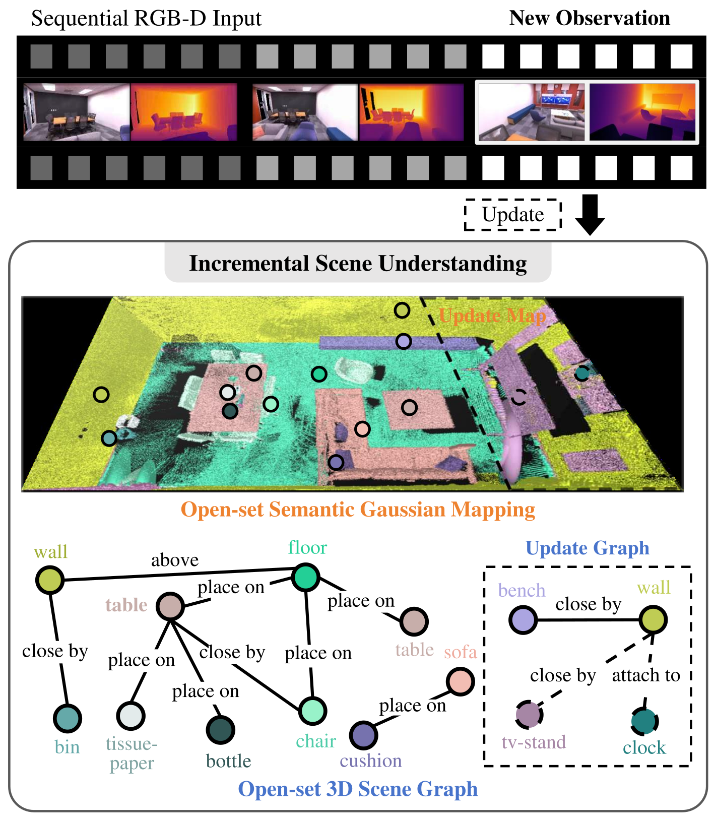
OGScene3D incrementally builds a Gaussian map and a scene graph from RGB-D observations. Its central idea is to maintain confidence in region labels, combine local associations with periodic global corrections, and reuse historical views to identify unreliable assignments. A vision-language model supplies entity descriptions and a language model predicts spatial relationships. Reported mapping gains are substantial on the evaluated indoor scenes, but 3D accuracy uses ground-truth poses and the runtime comparison excludes segmentation.
At a glance
The system combines confidence-weighted Gaussian semantics, hierarchical label refinement, a spatially selected memory of old observations, and selective graph updates. New views can correct existing entities as well as add new ones. Experiments cover Replica, ScanNet, four 3RScan scenes, and a quadruped demonstration. The evidence supports incremental indoor mapping and spatial relationship prediction, with functional relationships and end-to-end real-time deployment left for future work.
I Introduction
Robots exploring an environment need semantic maps and relationships before a complete scene reconstruction is available. Per-region feature vectors require later text matching, dense per-Gaussian embeddings consume memory, and single discrete labels can propagate segmentation errors. OGScene3D instead stores a region identifier and confidence per Gaussian, uses repeated observations to repair uncertain labels, and progressively creates textual entity descriptions and graph edges. Its memory revisits historical evidence so updates need not be confined to the currently visible region.
II Related Work
The related work separates geometric/semantic map representations from graph methods that describe objects and their relationships. The proposed combination targets open-vocabulary semantics during incremental reconstruction.
II-A 3D Representation and Semantic Mapping
Point, surfel, voxel, distance-field, mesh, radiance-field, and Gaussian maps offer different geometry, rendering, and storage trade-offs. Foundation models permit labels beyond a fixed training taxonomy, but their masks can disagree across views. ConceptGraphs and HOV-SG associate visual-language features with regions; Gaussian methods can store either dense features or compact labels. OGScene3D’s distinction is compact label-and-confidence storage combined with global and historical correction. Broad claims that earlier explicit maps cannot achieve high fidelity are motivation, not a controlled comparison of every representation.
II-B 3D Scene Graphs
A scene graph represents entities as nodes and spatial relationships as edges. Earlier methods include incremental closed-vocabulary graph prediction and foundation-model-based open-vocabulary descriptions, often built after mapping. This system updates open-vocabulary node descriptions and selected spatial edges as exploration proceeds; it does not expand the relationship model to functional or causal associations.
III Method
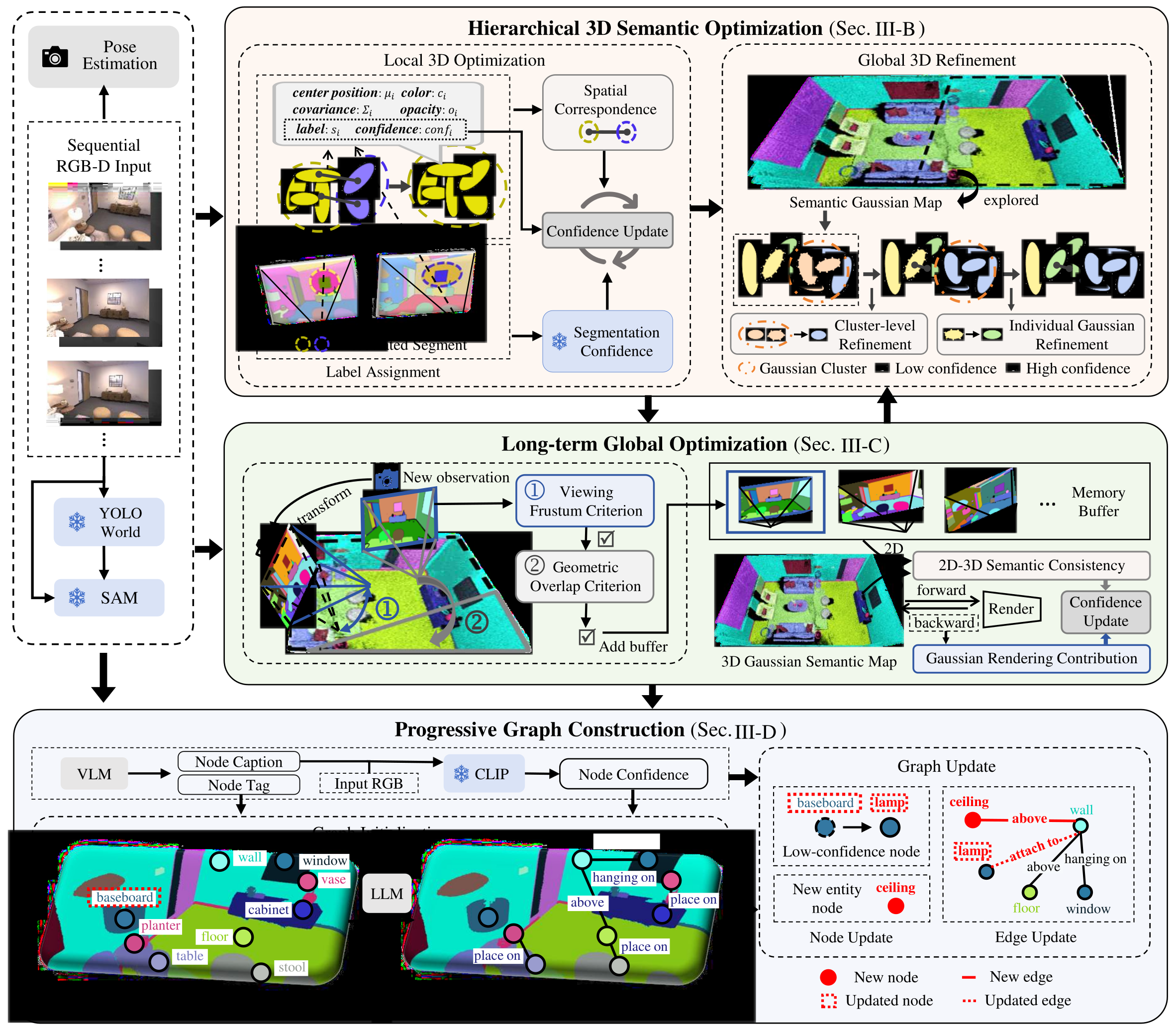
Given an RGB-D stream and estimated camera poses, the pipeline initializes and associates Gaussian regions, refines labels and confidence, revisits a memory buffer, and maintains a scene graph. Figure 2 preserves the interaction between mapping, temporal optimization, and graph construction.
III-A Confidence-based Scene Representation
Each Gaussian stores position, covariance, opacity, color, a discrete region label, and semantic confidence. Geometry and color use depth-ordered splatting; semantic rendering uses confidence-weighted class votes rather than numerically blending categorical IDs. Gaussians sharing a label form graph entities with a separate caption-confidence score. These IDs initially identify regions, not object names.
The source uses DROID-SLAM for incremental pose estimation. Confidence is an operational reliability weight, not a demonstrated calibrated probability. Keeping a scalar label and confidence avoids dense per-Gaussian language embeddings, although the full system also stores images, geometry, descriptions, and a history buffer.
Equations 1–3
| (1) |
| (2) | |||
| (3) |
III-B Hierarchical 3D Semantic Optimization
Hierarchical semantic optimization first establishes local segment correspondences, then periodically repairs unreliable labels across the map. A combined detector/segmenter supplies 2D regions; geometric association and confidence updates address cross-view disagreement.
III-B 1 Open-set Segmentation
Uniform-point prompting of SAM supplies broad region coverage. YOLO-World detections provide additional box prompts for more precise object masks. Fusion retains detection-guided masks and adds generic masks whose overlap with them is below 0.7. This trades detection precision against coverage of objects the detector misses; it does not eliminate segmentation errors.
III-B 2 Local 3D Optimization
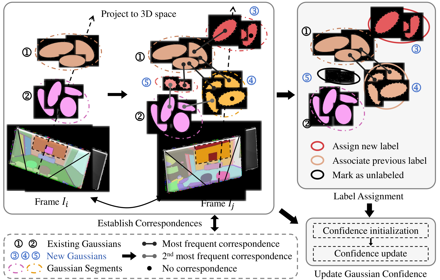
Depth back-projection initializes Gaussians from segmented keyframes. Nearest-neighbor matches to the current map are aggregated at segment level. The ratio of the second-most to most frequent matched label measures ambiguity, while the fraction supporting the dominant label measures correspondence coherence. Ambiguity of at least 0.25 leaves a segment unlabeled; otherwise coherence of at least 0.15 reuses the dominant label, and lower coherence creates a new region ID. Unlabeled Gaussians do not vote in semantic rendering.
Initial SAM confidence is linearly rescaled from the reported 0.88–1.0 range to 0.5–1.0. Matched, established labels gain confidence when new observations agree and lose it when they disagree, weighted by segmentation confidence and correspondence coherence. New or unlabeled regions do not update matched old-Gaussian confidence. The thresholds and rescaling are heuristic reliability controls rather than a calibration procedure.
Equations 4–5
| (4) |
| (5) |
III-B 3 Global 3D Refinement
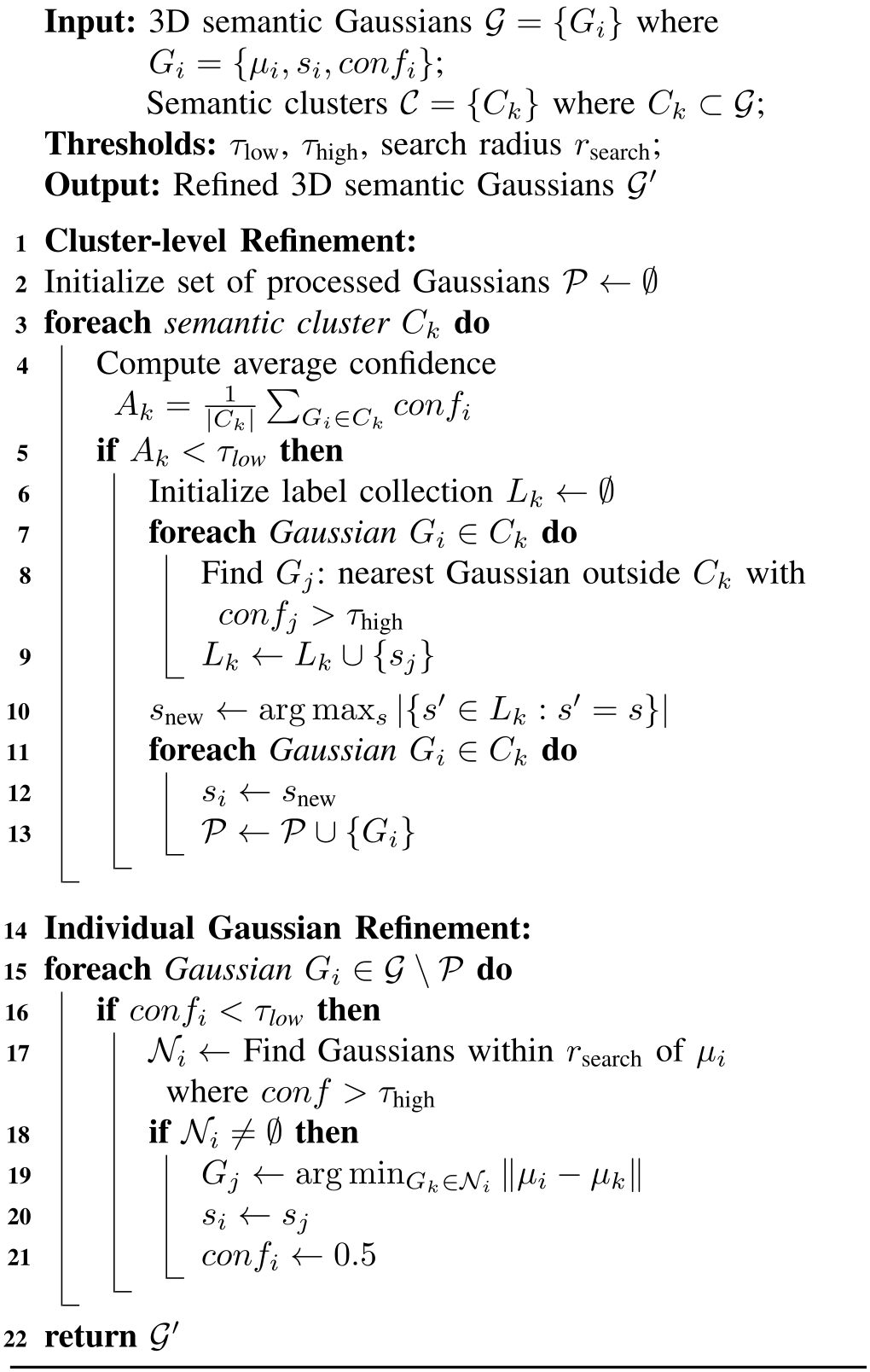
For each spatially connected same-label cluster, global refinement computes average confidence. A cluster below 0.3 adopts the most frequent label among nearest high-confidence neighbors outside the cluster; those neighbors must exceed 0.7. Cluster relabeling leaves individual confidences unchanged and records processed Gaussians.
Remaining low-confidence Gaussians may adopt the label of the closest high-confidence neighbor within radius 0.1; their confidence is reset to 0.5. Algorithm 1 preserves the exact ordering and no-neighbor condition. These operations propagate nearby reliable labels without changing geometry, but spatial proximity cannot guarantee correct object boundaries.
III-B 4 Loss Functions
Appearance and geometry use rendered RGB/depth reconstruction losses, separate from the discrete semantic-label rules. Color combines an L1 image term and structural-similarity loss with mixture weight 0.2; depth uses an L1 term. Their overall weights are 1 and 0.1. Adam optimizes Gaussian parameters; the method does not differentiate arbitrary categorical region numbers as continuous semantic values.
Equations 6–7
| (6) |
| (7) |
III-C Long-term Global Optimization
A memory of representative old views lets the system reassess areas absent from recent observations. Long-term optimization updates confidence, leaving direct relabeling to the global-refinement stage. It combines agreement between stored 2D masks and rendered labels with each Gaussian’s contribution to an auxiliary confidence rendering.
III-C 1 Memory Buffer Construction
A keyframe enters memory only when less than half its back-projected points lie in the most recent memory view’s frustum and less than half overlap geometry already represented by the entire buffer. The conjunction seeks both a distinct view and additional spatial coverage. The selected frames retain observations and viewpoints for later updates; this selection does not establish a fixed memory-size bound.
Equations 8–9
| (8) |
| (9) |
III-C 2 2D-3D Semantic Consistency
Rendered map labels are compared with remapped SAM masks from a stored view using class-wise intersection over union. Each pixel inherits its class’s agreement score, then depth projection and nearest-neighbor association transfer that score to Gaussians. This measures consistency with the segmenter’s historical evidence, not correctness against ground-truth labels: repeated systematic segmentation mistakes may still agree.
Equations 10–11
| (10) |
| (11) |
III-C 3 Gaussian Rendering Contribution
An auxiliary semantic rendering weights one-hot vectors using both Gaussian opacity and semantic confidence, with depth-ordered transmittance. The ratio between gradients of squared and linear rendered-value losses estimates a Gaussian’s influence, with a small denominator stabilizer. This carries geometric visibility and semantic reliability into the confidence update. Gradients provide the weighting signal, while semantic labels remain discrete.
Equations 12–15
| (12) |
| (13) |
| (14) |
| (15) |
III-C 4 Long-term Confidence Update
For historically consistent labels, the update raises confidence by a term weighted by 2D–3D agreement, rendering contribution, and remaining headroom. For inconsistent labels, it reduces confidence using agreement and the complementary contribution factor. These bounded-style updates can flag uncertain historical regions for subsequent relabeling, without directly changing their labels during this stage.
Equation 16
| (16) |
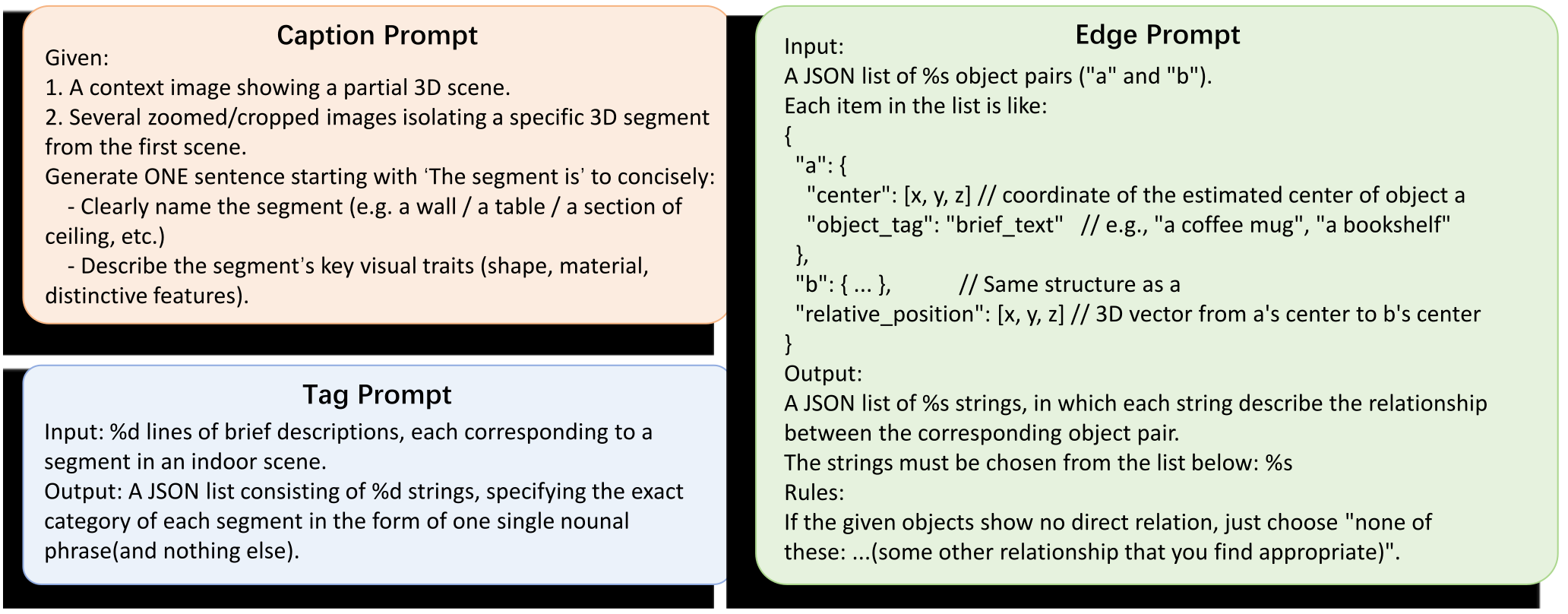
III-D Progressive Graph Construction
Scene regions receive natural-language captions and tags, while spatially adjacent entities receive graph edges. This converts anonymous map IDs into interpretable objects and structural elements such as walls. Graph initialization and confidence-triggered updates use different schedules from Gaussian refinement.
III-D 1 Graph Initialization
The first twelve keyframes initialize the graph. Each entity is represented by its largest contextual crop and three largest masked views, using fewer views when necessary. GPT-4o generates a caption; CLIP measures crop–caption alignment as node confidence. This score indicates semantic similarity rather than verified caption truth.
Candidate edges require a sufficient fraction of one entity’s points to lie within distance 0.1 of the other; the maximum of the two directional fractions must exceed 0.2. GPT-4o receives entity tags, centers, and relative position vectors to describe relationships, batching candidate pairs into one call. Captions are open vocabulary, while relationships favor a common spatial-relation list with limited fallback flexibility. Figure 4 retains the exact caption, tag, and edge prompts.
Equations 17–23
| (17) |
| (18) |
| (19) |
| (20) |
| (21) |
| (22) |
| (23) |
III-D 2 Graph Update
New entities and existing nodes with caption confidence below 0.3 are selected for updates. Larger, better-exposed views replace earlier crops/masks before recaptioning. Only edges incident to selected nodes are reconsidered, using the same proximity filter and batched language-model inference. This reduces repeated calls, while a confident but incorrect caption may evade the selection rule.
Equations 24–25
| (24) |
| (25) |
IV Experiments
Experiments evaluate rendered and 3D semantic segmentation, spatial relationship recall, qualitative real-robot mapping, processing time, and the two refinement components. The evaluation conditions matter when interpreting accuracy and online operation.
IV-A Experimental Setup
The study specifies a small set of indoor scenes, semantic and graph metrics, representation-dependent baselines, and fixed optimization schedules. Ground-truth poses and language-based output alignment are used in the 3D comparison.
IV-A 1 Datasets
Segmentation uses eight Replica scenes and five ScanNet scenes with semantic annotations. Relationship evaluation selects four 3RScan scenes with annotated edges. Additional indoor recordings from a quadruped test practical mapping qualitatively. These experiments do not establish performance over a broad outdoor, dynamic, or long-duration distribution.
IV-A 2 Evaluation Metrics
Semantic metrics are mean intersection over union, frequency-weighted mean intersection over union, and mean class accuracy, reported as percentages. Graph evaluation reports relationship recall. The paper does not provide a comparable precision metric for predicted edges, so recall gains alone do not quantify false-positive behavior.
IV-A 3 Baselines
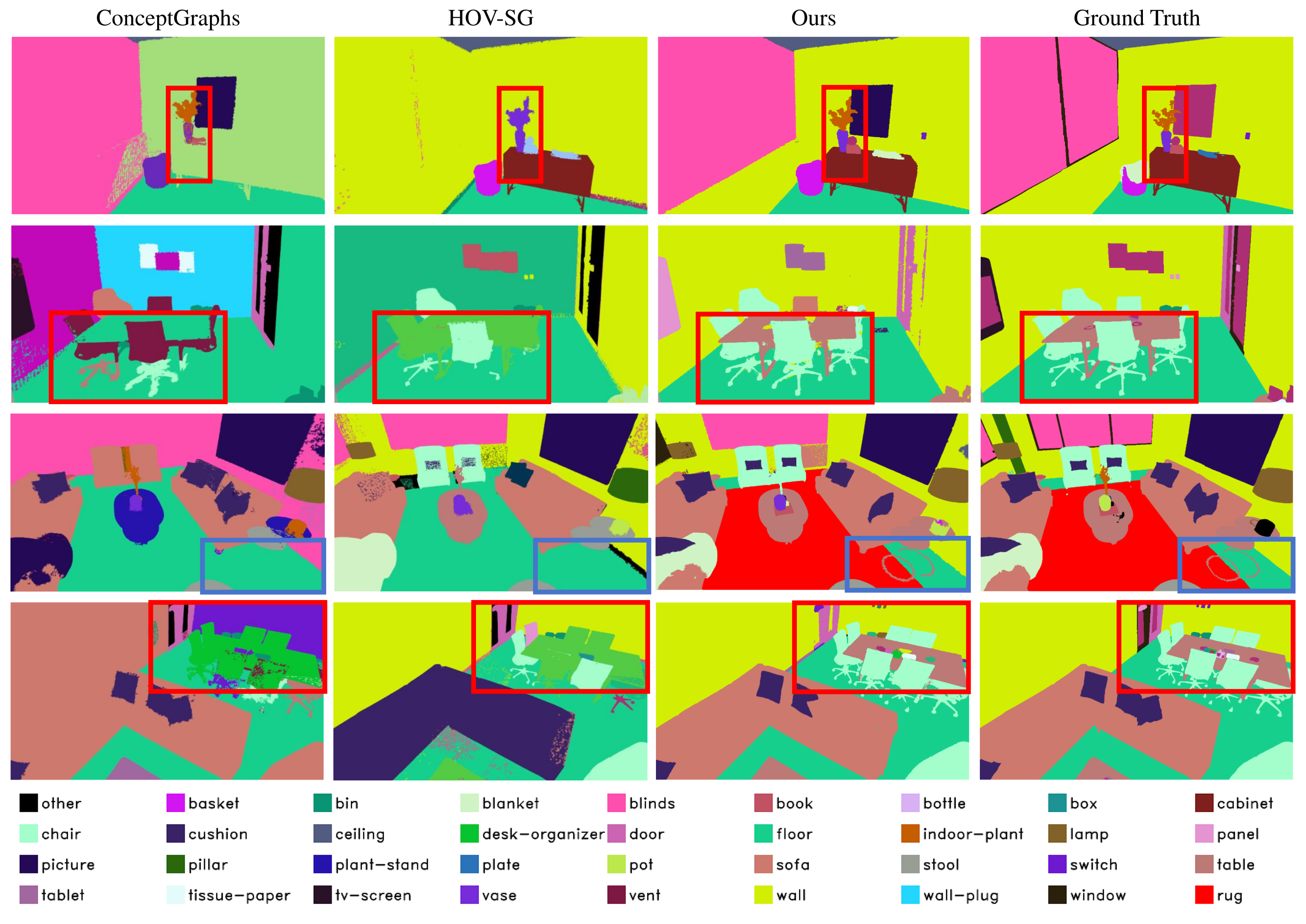
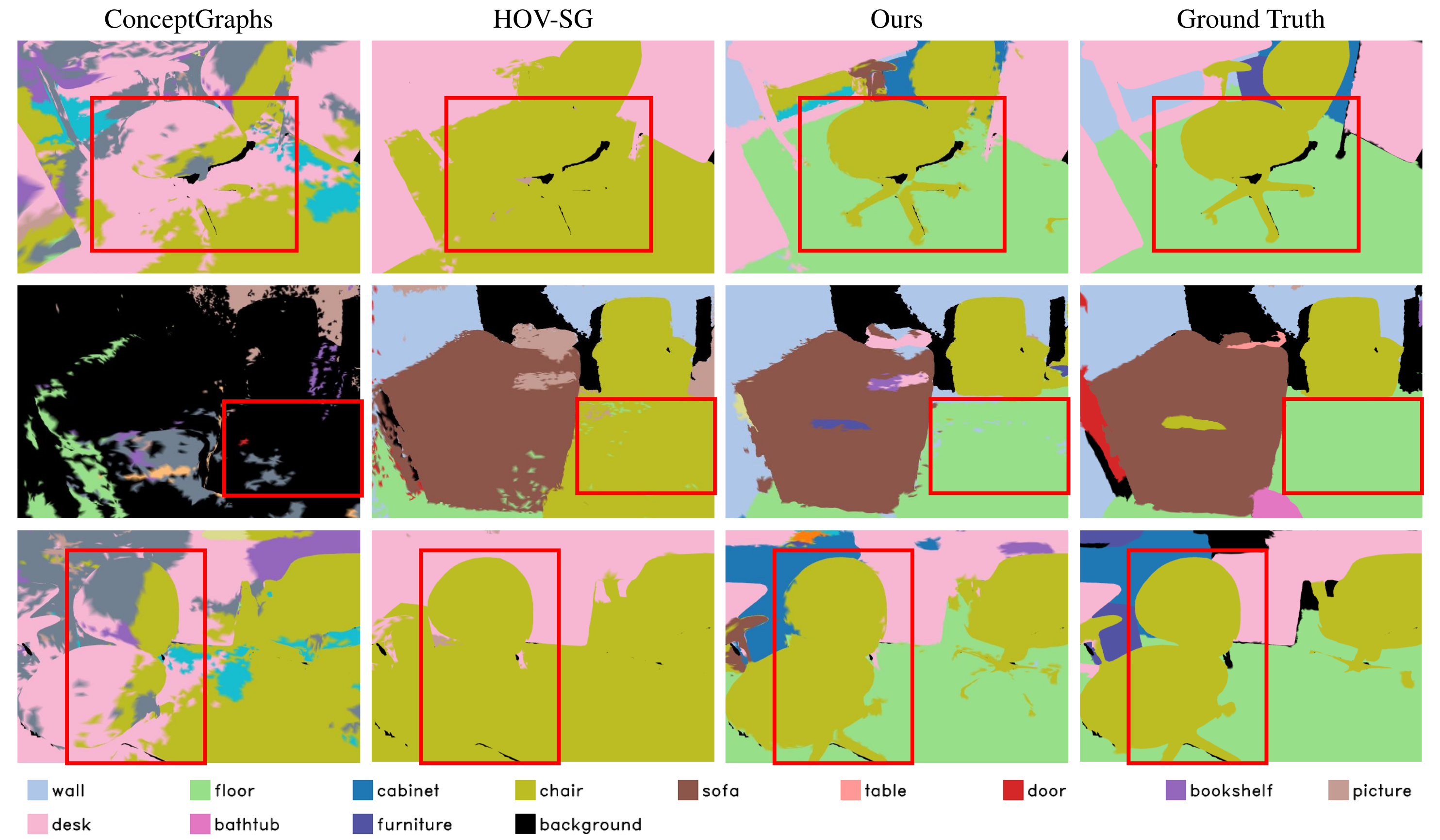
Table I compares novel-view segmentation with Feature 3DGS, GS-Grouping, and OpenGS-SLAM. The 3D comparison uses ConceptGraphs and HOV-SG, while relationship evaluation uses an extended ConceptGraphs relation vocabulary. Figures 5–6 label their qualitative columns ConceptGraphs and HOV-SG, so their displayed baselines differ from the quantitative methods in Table I. ScanNet baseline values are taken from the HOV-SG paper rather than all being rerun in this evaluation.
IV-A 4 Implementation Details
High/low Gaussian-confidence thresholds are 0.7/0.3. Global refinement and historical optimization run every six keyframes; graph updates run every twelve. Local association uses ambiguity 0.25, coherence 0.15, and radius 0.1; memory inclusion requires both overlap measures below 0.5. Gaussian learning rates are 0.001 for scales, 0.05 for opacity, and 0.0001 for color. Main experiments use an RTX 4090, while the robot demonstration uses an RTX 3080 laptop.
| Methods | Metrics | room0 | room1 | room2 | office0 | office1 | office2 | office3 | office4 | Avg. |
|---|---|---|---|---|---|---|---|---|---|---|
| Feature 3DGS [57] | mIoU | 49.62 | 47.71 | 53.00 | 51.37 | 44.94 | 49.49 | 48.93 | 46.06 | 48.89 |
| mAcc | 59.46 | 55.37 | 62.21 | 59.42 | 52.19 | 58.25 | 57.84 | 55.36 | 57.51 | |
| GS-Grouping [58] | mIoU | 60.55 | 57.68 | 62.82 | 63.42 | 55.41 | 59.33 | 57.91 | 56.05 | 59.15 |
| mAcc | 69.02 | 67.83 | 71.41 | 73.61 | 66.78 | 71.51 | 70.29 | 69.06 | 69.94 | |
| OpenGS-SLAM [10] | mIoU | 64.06 | 61.18 | 64.38 | 61.53 | 58.11 | 63.05 | 62.71 | 60.25 | 61.91 |
| mAcc | 73.53 | 72.13 | 74.17 | 73.05 | 69.03 | 75.36 | 73.62 | 74.01 | 73.11 | |
| OGScene3D (Ours) | mIoU | 67.94 | 65.96 | 71.23 | 70.82 | 74.08 | 72.99 | 75.57 | 75.58 | 71.77 |
| mAcc | 91.33 | 87.71 | 83.60 | 92.73 | 92.88 | 83.08 | 90.85 | 91.04 | 89.15 |
IV-B Semantic Mapping Evaluation
Mapping is assessed both by rendering semantic labels into novel views and by assigning labels to 3D geometry. Colors in the retained figures denote categories; they are visualization aids rather than a shared numerical encoding across all scenes.
IV-B 1 2D Semantic Segmentation
On Replica novel views, average mIoU is 71.77 versus 61.91 for the strongest listed baseline, OpenGS-SLAM; mean accuracy is 89.15 versus 73.11. These are gains of 9.86 and 16.04 percentage points, approximately 16% and 22% relative improvements. The original table preserves every scene. Qualitative examples show improved separation of plants, furniture, fine legs, and background surfaces, but these selected views do not independently measure generalization.
| Methods | Metric | room0 | room1 | room2 | office0 | office1 | office2 | office3 | office4 | Avg. |
|---|---|---|---|---|---|---|---|---|---|---|
| ConceptGraphs [1] | mIoU | 12.35 | 14.04 | 10.58 | 20.23 | 11.61 | 19.08 | 9.71 | 22.04 | 14.95 |
| F-mIoU | 21.20 | 15.75 | 27.16 | 32.20 | 11.54 | 25.85 | 11.64 | 42.44 | 23.47 | |
| mAcc | 27.08 | 34.68 | 27.34 | 31.73 | 31.49 | 29.27 | 26.73 | 41.22 | 31.19 | |
| HOV-SG [2] | mIoU | 33.74 | 27.37 | 18.27 | 24.81 | 11.93 | 20.98 | 19.95 | 27.37 | 23.05 |
| F-mIoU | 62.77 | 40.84 | 43.78 | 33.78 | 17.78 | 40.51 | 26.00 | 43.58 | 38.63 | |
| mAcc | 43.57 | 39.22 | 26.18 | 28.17 | 23.88 | 24.99 | 28.46 | 28.72 | 30.40 | |
| OGScene3D (Ours) | mIoU | 39.87 | 36.07 | 31.63 | 28.83 | 17.56 | 25.67 | 25.96 | 35.71 | 30.16 |
| F-mIoU | 53.23 | 42.22 | 40.68 | 28.02 | 22.78 | 54.32 | 51.32 | 54.69 | 43.41 | |
| mAcc | 51.63 | 55.16 | 49.93 | 40.58 | 37.01 | 30.53 | 30.57 | 41.46 | 42.11 |
| Methods | Metric | scene0011_00 | scene0050_00 | scene0231_00 | scene0378_00 | scene0518_00 | Avg. |
|---|---|---|---|---|---|---|---|
| ConceptGraphs [1] | mIoU | – | – | – | – | – | 16.00 |
| F-mIoU | – | – | – | – | – | 20.00 | |
| mAcc | – | – | – | – | – | 28.00 | |
| HOV-SG [2] | mIoU | 27.80 | 17.23 | 22.72 | 26.67 | 16.58 | 22.20 |
| F-mIoU | 42.19 | 36.50 | 26.39 | 29.15 | 17.27 | 30.30 | |
| mAcc | 44.59 | 41.62 | 40.50 | 51.28 | 37.51 | 43.10 | |
| OGScene3D (Ours) | mIoU | 31.47 | 28.54 | 25.35 | 37.70 | 24.13 | 29.44 |
| F-mIoU | 42.33 | 50.53 | 26.93 | 38.61 | 23.29 | 36.34 | |
| mAcc | 55.55 | 40.77 | 42.21 | 58.46 | 35.05 | 46.41 |
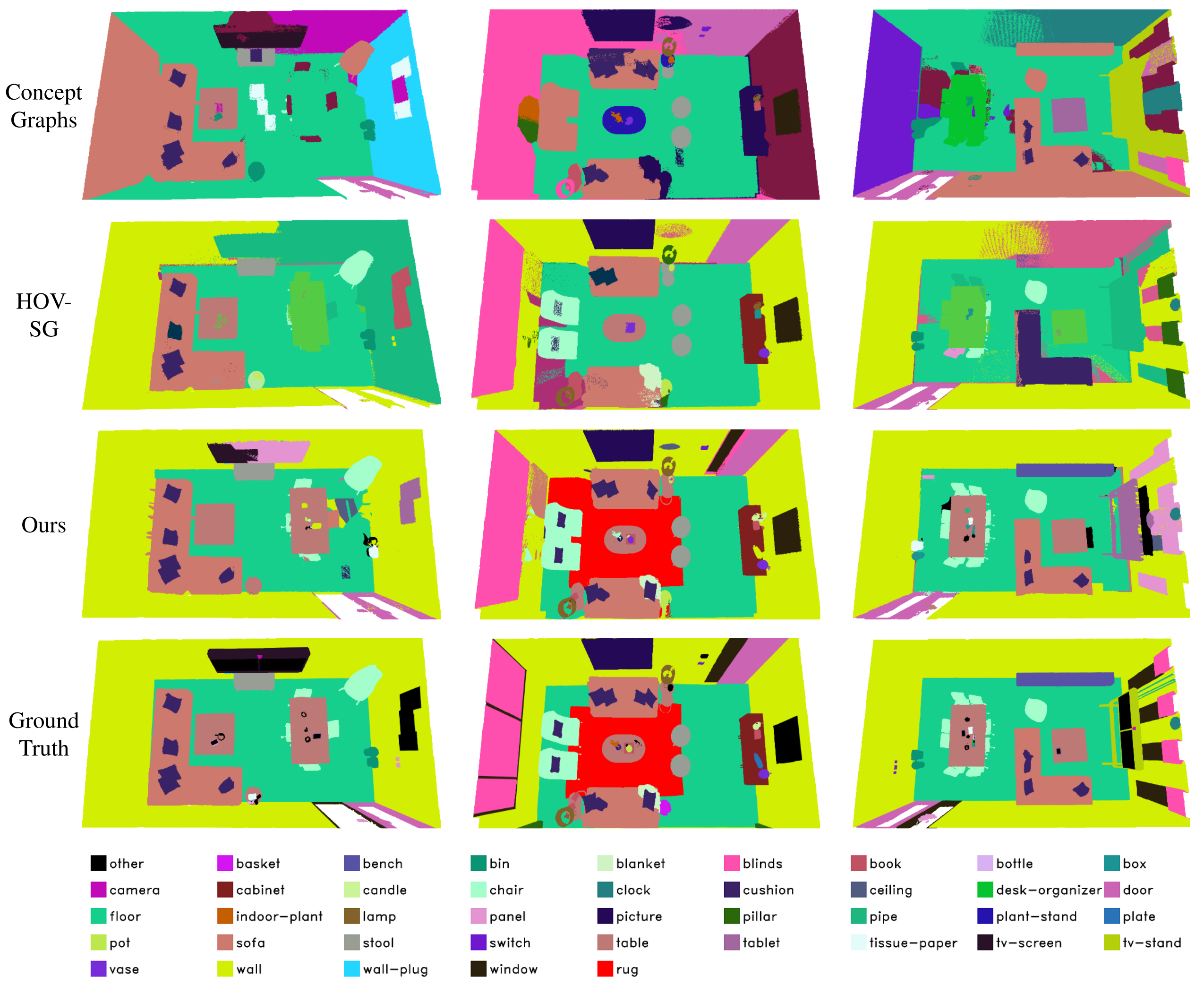
IV-B 2 3D Semantic Segmentation
For 3D evaluation, all compared maps use ground-truth poses. Gemma aligns OGScene3D’s generated descriptions with benchmark labels, while feature-based baselines use text-feature similarity. Replica averages are 30.16 mIoU, 43.41 frequency-weighted mIoU, and 42.11 mean accuracy; HOV-SG reaches 23.05, 38.63, and 30.40 respectively. ScanNet averages are 29.44, 36.34, and 46.41, versus HOV-SG’s 22.20, 30.30, and 43.10.
The average improvements do not imply winning every metric in every scene: some weighted-IoU and class-accuracy entries favor baselines. ScanNet’s ConceptGraphs values are reported only as averages. Ground-truth poses and different semantic-alignment procedures limit conclusions about fully online tracking-and-mapping accuracy. The source says segmentation inputs are shared, but later label processing remains method-specific.
| Methods | 137a8158 | 10b17940 | bf9a3dd3 | 0988ea72 |
|---|---|---|---|---|
| ConceptGraphs [1] | 2.5 | fail | 3.5 | 0.9 |
| OGScene3D (Ours) | 28.7 | 25.6 | 22.8 | 18.3 |
IV-C Scene Graph Evaluation
Across the four 3RScan scenes, OGScene3D’s relationship recall is 28.7%, 25.6%, 22.8%, and 18.3%. ConceptGraphs obtains 2.5%, a reported failure, 3.5%, and 0.9%, after its relation vocabulary is expanded to the dataset’s range. These are clear gains on the selected scenes, while absolute recall remains limited and the failed baseline case should not be silently converted into a measured zero.
IV-D Real World Experiment
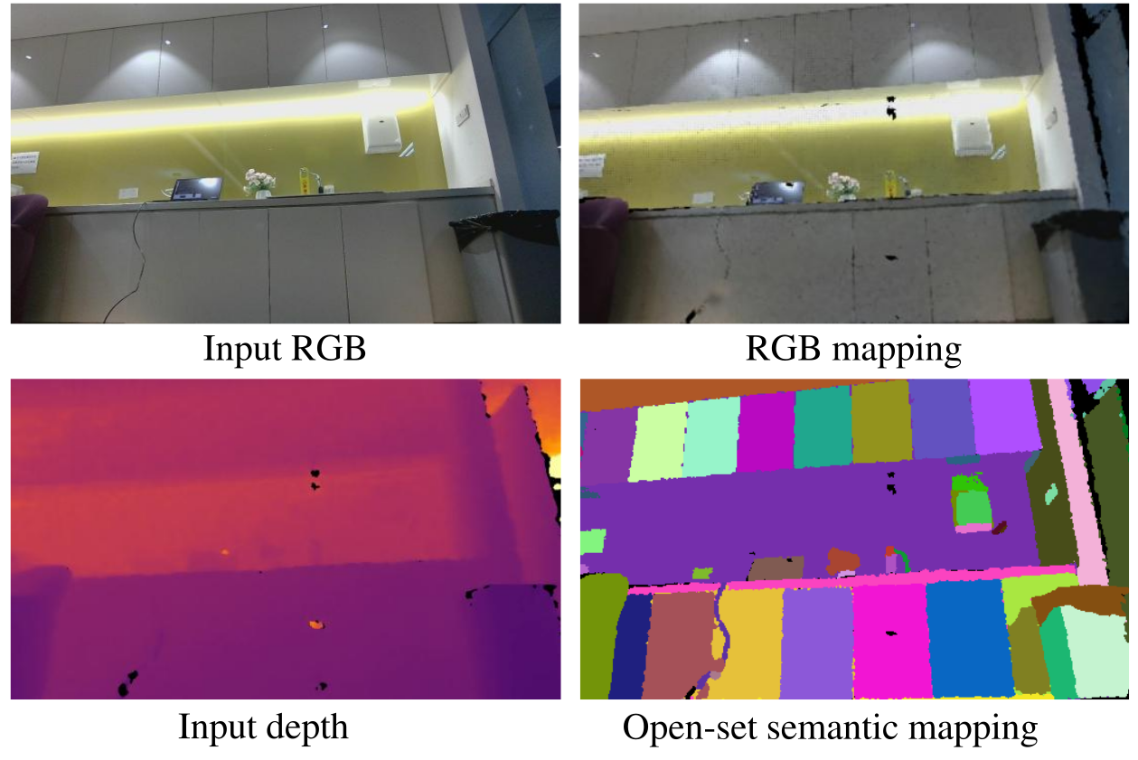
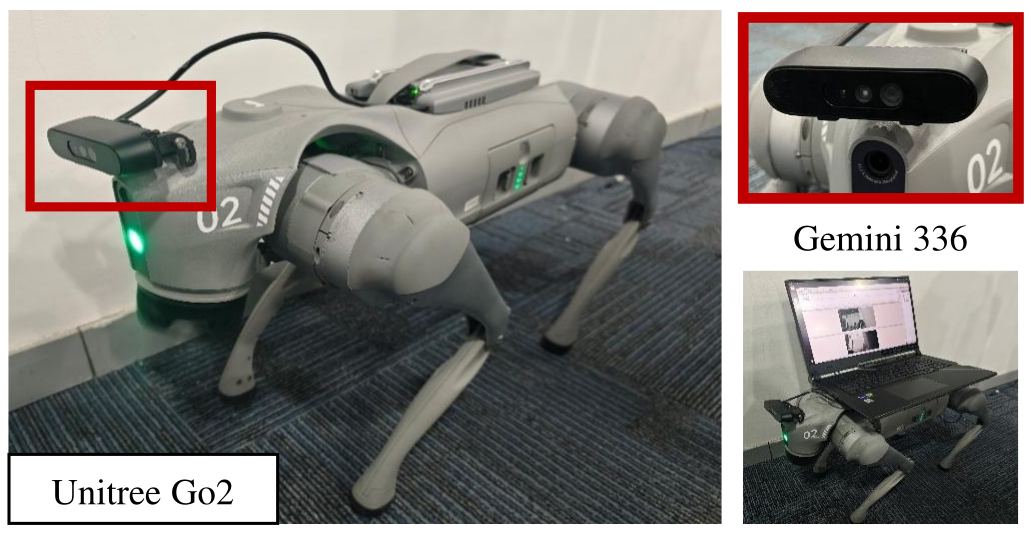
A Unitree Go2 carries a Gemini 336 RGB-D camera while an RTX 3080 laptop performs mapping and scene understanding. Figures 8–9 show reconstructed appearance, semantic regions, and hardware. The reported demonstration is qualitative; the paper directs readers to a video but does not supply a robot task-success or quantitative real-world relationship score here.
IV-E Runtime Analysis
Reported ScanNet mapping time is 10 min 13 s per scene, versus 31 min 56 s for HOV-SG and 122 min 5 s for ConceptGraphs. SAM segmentation time is explicitly excluded. Averaged module costs are 0.248 s for local optimization, 0.055 s for global refinement, and 0.020 s for historical optimization, totaling 0.323 s per frame. These mapping measurements do not establish end-to-end real-time operation with segmentation, pose estimation, and language-model graph calls included.
IV-F Ablation Study
The ablations retain local association because removing it would prevent the basic mapping pipeline from functioning. Table VII then adds global refinement and historical optimization sequentially; these results isolate incremental components within that retained framework.
IV-F 1 Effectiveness of Hierarchical 3D Semantic Optimization
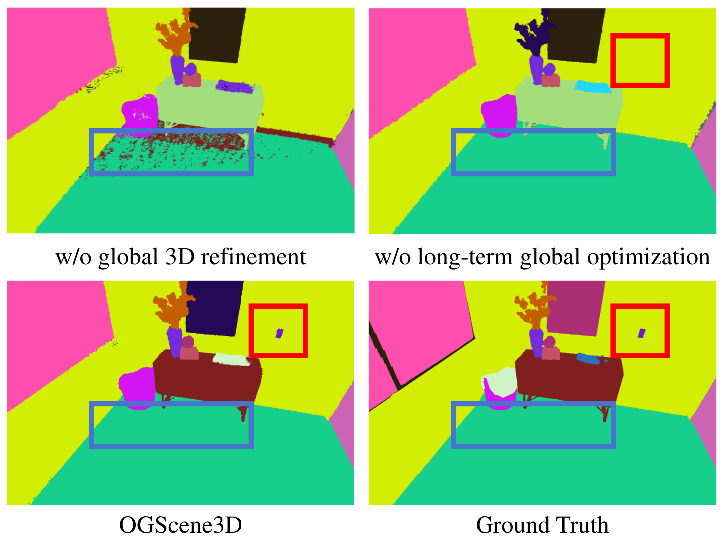
Table VII reports local-only mIoU of 22.98, rising to 25.35 after global refinement; frequency-weighted mIoU rises from 35.15 to 38.16, and mean accuracy from 42.85 to 49.02. Blue boxes in Figure 10 illustrate residual noisy regions without refinement. The prose incorrectly associates removing global refinement with row (b); the table explicitly defines row (a) as local-only and row (b) as adding refinement. These are the reported ablation values, not the eight-scene aggregate in Table II.
IV-F 2 Effectiveness of Long-term Global Optimization
Adding long-term optimization raises the ablation setting to 36.07 mIoU, 42.22 frequency-weighted mIoU, and 55.16 mean accuracy. Figure 10’s switch example shows how historical close views can help retain a small entity missed in distant observations. The evidence supports the combined memory/confidence module, without separately identifying the contribution of each memory-selection or gradient-weighting choice.
V Conclusion and future work
The conclusion emphasizes incremental semantics and graph maintenance; the stated future direction extends spatial relations toward richer relational understanding and real-time deployment.
V-A Conclusion
Confidence-guided association, periodic relabeling, historical consistency, and selective graph updates form a coherent incremental mapping pipeline. The retained experiments show improvements on the chosen indoor benchmarks and a robot recording. Suggested applications in planning, contextual queries, and augmented reality remain prospective rather than separately evaluated downstream tasks.
V-B Limitation and Future Work
The authors identify spatial-only relationships as a principal limitation and propose functional associations and broader multi-relational scene understanding. Additional limits evident from the protocol include dependence on foundation-model masks and captions, heuristic confidence thresholds, ground-truth poses for 3D evaluation, a small relation benchmark, and runtime exclusions. Reliable real-time robotic deployment therefore requires further evaluation beyond the presented mapping results.