At a glance
Low-frequency position-only VLA commands can make a compliant robot lag behind its target. This paper supplies target velocity through finite differences or a learned cubic B-spline action representation, while retaining the policy architecture. On one cube-in-hole task, finite differences reduce reported completion time from 7.35 to 6.05 seconds. Splines reach a reported 79.20% final success rate but do not significantly improve execution time. Acceleration feedforward is proposed, not tested.
I Introduction
Active compliance lets rigid manipulators yield during contact. With only position setpoints, accurate tracking depends strongly on stiffness; lowering stiffness increases lag. Supplying the desired velocity addresses a different issue from choosing when to lower stiffness. The motivation follows classical impedance control, while learned compliance methods such as Adaptive Compliance Policy modify interaction behavior.
The contribution is the connection between a VLA action interface, demonstration collection and the fast controller. Finite differences and B-splines themselves are established methods. The authors claim broad architectural compatibility, but evaluate only one fine-tuned policy family. This edition covers all six pages of the 17 March 2026 v1 and preserves all six figures, two tables, seven numbered equations and 30 references.
II Methodology
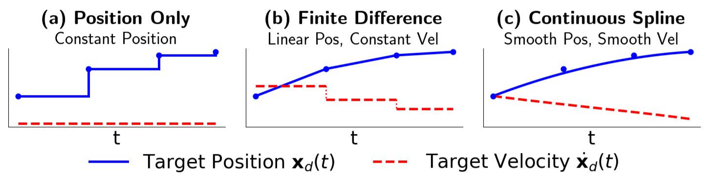
An action-chunking policy maps images, language and robot state to a future action sequence. The baseline sends discrete positions with zero desired velocity. The first proposed interface derives velocity from successive position targets; the second predicts control points defining a continuous curve. Neither requires changing the neural-network architecture, but both change the data/controller interface.
II-A Cartesian Compliance and Feedforward Dynamics
The intended compliant behavior is a mass–spring–damper relation between tracking error and external force. Desired inertia, damping and stiffness govern the response. Position-only targets omit the feedforward velocity, so the stiffness-related position error must supply much of the motion command. Cartesian admittance is the implemented example; torque-level impedance and joint-space compliance are suggested applications.
Finite differences approximate target velocity by (xₜ−xₜ₋₁)/Δt, corresponding to piecewise-linear target position and piecewise-constant velocity. This is compatible with discrete action chunks, but velocity jumps remain at segment boundaries. Crucially, demonstrations must use the same velocity-aware controller as deployment; simply switching the controller under an existing dataset can create a mismatch.
The printed equations contain a sign inconsistency. Given e=xd−x, rearranging Equation 1 gives ẍ=ẍd+Λd⁻¹(Ddė+Kde−Fext), whereas Equation 2 prints a minus before the inverse-inertia term. Both originals are preserved. The paper does not establish whether that typographical inconsistency appears in the actual implementation. Inverting Λd also requires nonsingularity, beyond merely calling it positive semidefinite.
Equations 1–2
| (1) |
| (2) |
II-B Method 2: Cubic B-Spline Action Space
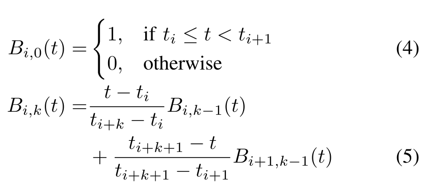
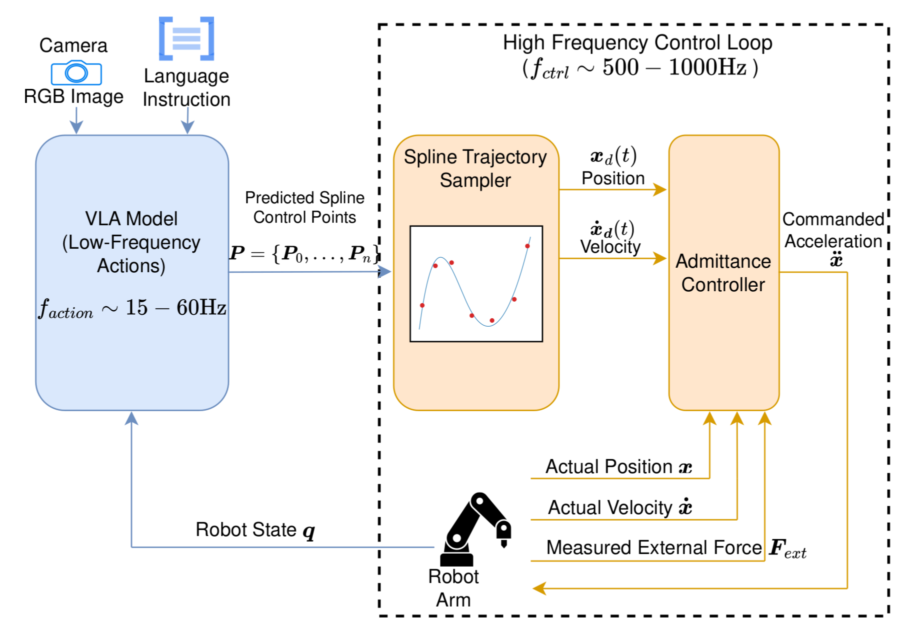
The spline policy predicts control points Pᵢ, and the controller evaluates their weighted sum using degree-three B-spline basis functions. The standard basis recursion makes position, velocity and acceleration analytically available; on ordinary cubic spans, only four control points contribute. The conceptual workflow separates low-frequency action generation from the fast control loop.
Training targets come from least-squares fitting of the full high-frequency demonstration trajectory, followed by extracting local control-point targets for observations. The method retains standard behavior cloning. Figure 2 illustrates action rates around 15–60 Hz and control rates around 500–1000 Hz; these schematic ranges are not a complete specification of the evaluated configuration.
C² continuity requires appropriate knot multiplicities and applies within a spline, not automatically between independently predicted chunks. The experiment later reports residual chunk-boundary jerks. Knot placement, fit constraints, pose/orientation handling and boundary-matching details are insufficiently specified for exact reproduction. Although second derivatives are available analytically, the experiments set desired acceleration to zero.
Equations 3–7
| (3) |
Original selectable MathML
| (4) | ||||
| (5) |
| (6) | ||||
| (7) |
III Results
The evaluation separates human teleoperation from learned-policy rollout. Completion time and success over a 20-second horizon assess the balance between fast transfer and compliant insertion. They do not directly measure contact-force limits, damage risk or tracking-error trajectories.
III-A Experiment Setup
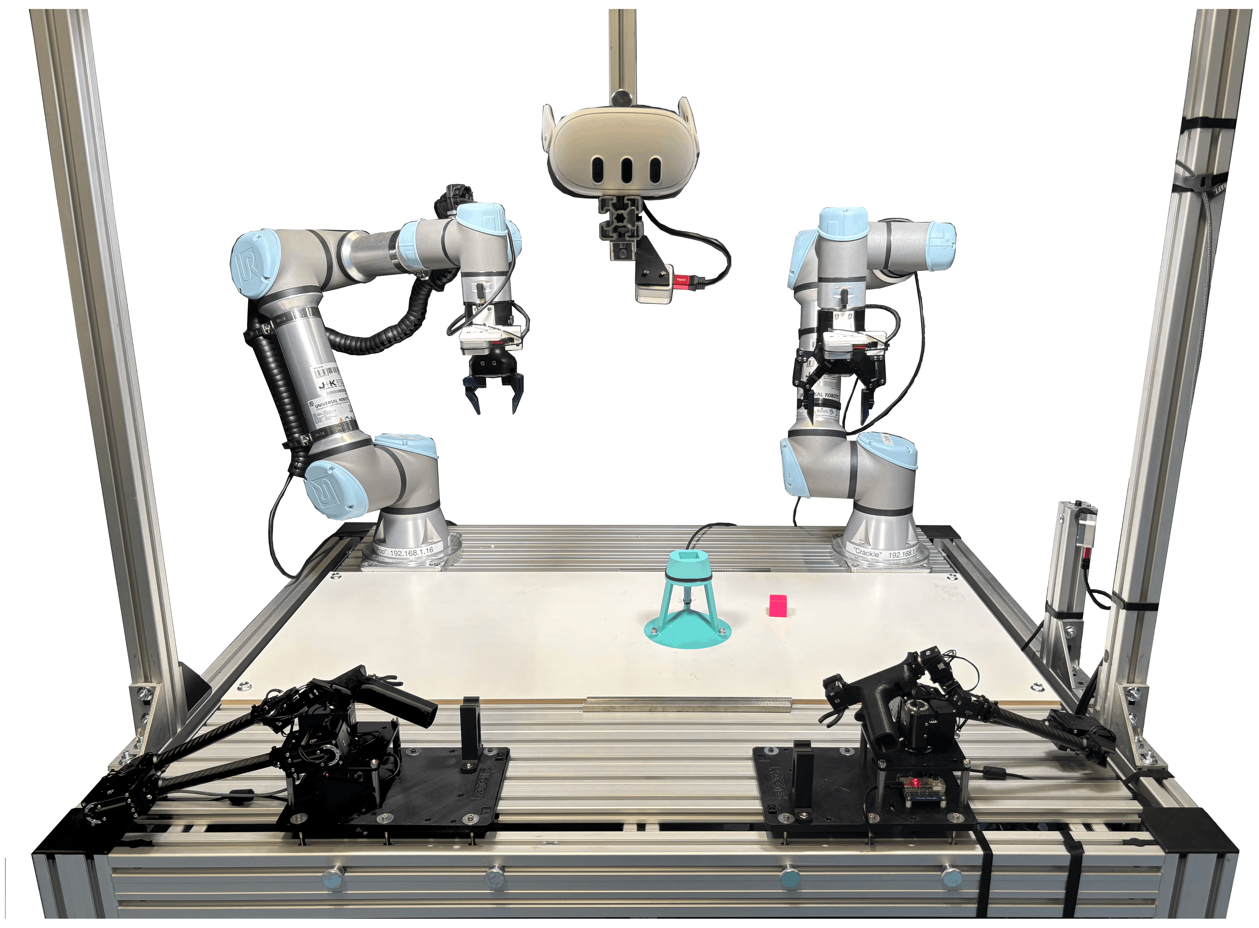
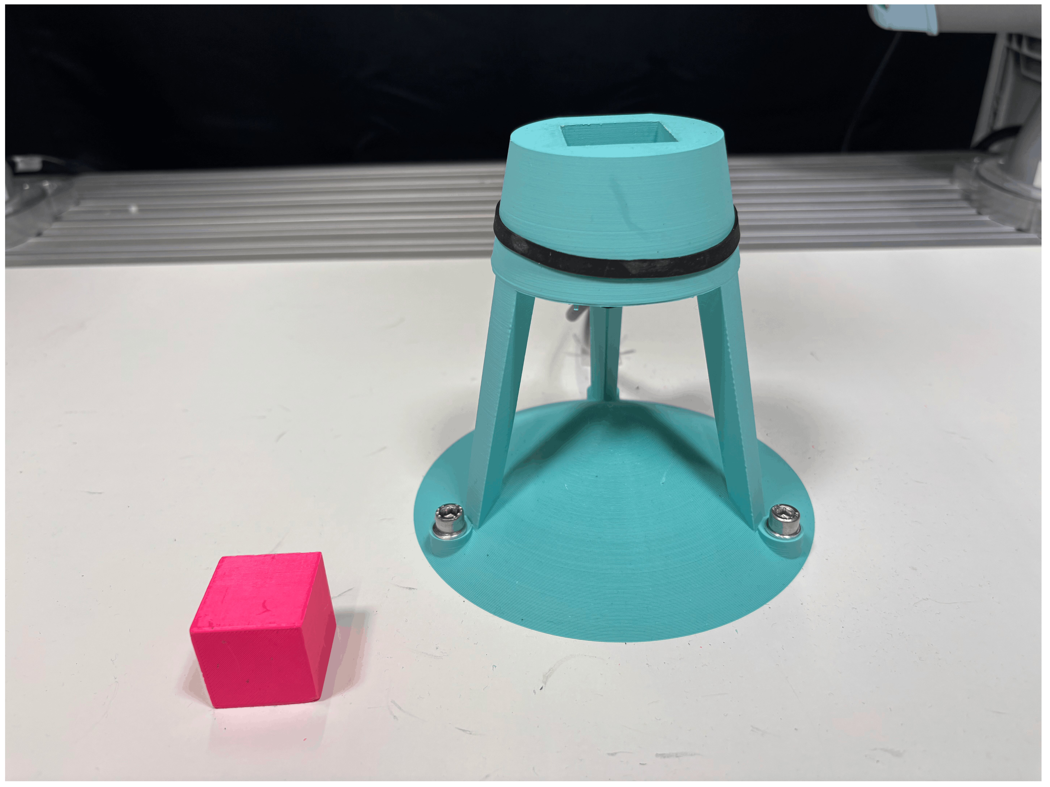
Two Universal Robots arms and two OMY-L100 teleoperation devices perform cube insertion into a plastic fixture with a 1 mm margin. After insertion, the cube drops onto a cone and lands at a random workspace location, creating a subsequent transfer motion. Teleoperation samples desired position above 500 Hz; low-pass-filtered finite differences supply velocity. Acceleration is omitted because double differentiation amplifies noise.
The controller uses ur_rtde. Each π₀.₅ model is fine-tuned for 40,000 steps with batch size 32. real-time chunking uses flow-policy inpainting to reduce discontinuities during inference. The paper does not report demonstration-set size, numerical compliance gains, complete action/control timing or trial allocation across arms. Demonstrating a successful compliant task is weaker evidence than a measured force/safety guarantee.
III-B Teleoperation Results
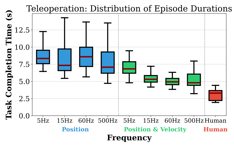
A human operator works in nominal 10-minute intervals, prioritizing speed rather than constructing a structured training set. At reference rates of 5, 15, 60 and 500 Hz, mean completion times fall from 9.58→7.64, 8.48→5.85, 9.31→5.34 and 8.37→5.37 seconds when adding velocity. Table I retains all dispersions, sample sizes and one-sided t-tests; each comparison reports p<0.001.
Velocity-aware operation remains slower at 5 Hz than at higher rates, consistent with increased sensitivity to delayed targets. Position-only operation changes less with frequency. Figure 5 also shows a human-only comparison, but its sampling protocol is not detailed. Repeated completions from a human-operated session are not independent operators or randomized replications; session pooling, counterbalancing and uncertainty beyond the t-tests are not documented. These timing results establish an observed advantage in this setup, rather than directly quantifying tracking accuracy.
| Frequency | Position (Baseline) | Position & Velocity (Method) | -statistic | -value |
|---|---|---|---|---|
| () | () | |||
| () | () | |||
| () | () | |||
| () | () |
III-C Policy Task Execution Speed
Table II reports baseline mean/variance/N of 7.35 s/1.99/71; finite differences give 6.05 s/1.71/70, with t=−5.70 and p<0.001. The 1.30-second reduction is about 17.7% of the baseline mean. Splines give 7.45 s/4.75/94, with p=0.626 for a decrease: no significant speed improvement, and greater time variance.
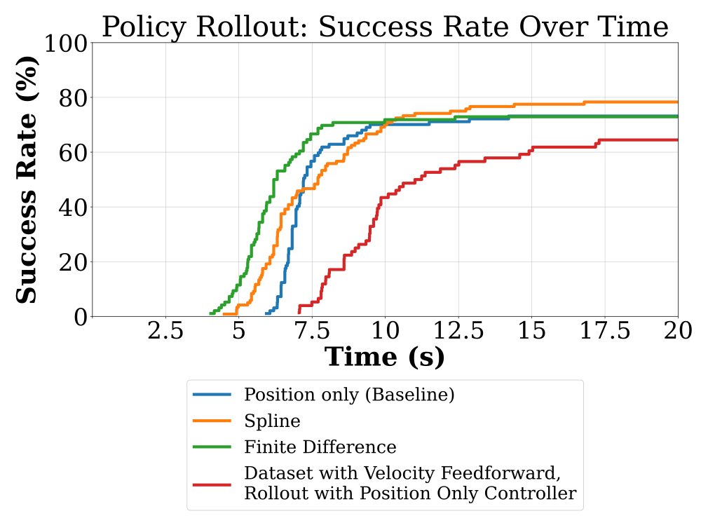
The spline policy reaches a reported 79.20% success by 20 seconds. Figure 6 preserves the complete cumulative curves: finite differences achieve early successes fastest, while spline completions continue later. The paper does not tabulate exact final percentages for all other conditions, total rollout denominators or confidence intervals; Table II N values are not clearly reconciled with the success curves. Completion-time means should not be interpreted as failure-penalized overall throughput without a specified censoring/reset protocol.
Residual discontinuities after real-time chunking can produce large spline-derived velocity commands and jerky motion. The authors hypothesize that this causes helpful insertion “wiggling,” explaining the high final success rate, but provide no dedicated force or motion ablation to test that mechanism. Smooth cubic spans therefore do not establish globally smooth closed-loop execution.
Training on velocity-aware demonstrations but rolling out a position-only controller gives 10.01 s, variance 6.10 and N=49; its one-sided test instead asks whether time increases and reports p<0.001. It also has the lowest plotted final success. This supports matching collection and deployment interfaces in this setup, not universal architectural compatibility or an isolated effect independent of the dataset change.
| Method | Mean (s) | Var. | -stat | -value∗ | Sig. () | |
| Baseline | – | – | – | |||
| Finite Difference | Yes | |||||
| Cubic B-Spline | No | |||||
| Ablation (Velocity-Feedforward Dataset, | ||||||
| Position Only Rollout) | Yes | |||||
| ∗ One-tailed -value testing for a decrease in execution time compared to the baseline. For the ablation we instead test for an increase in execution time. | ||||||
IV Conclusion and Future Work
The practical result is a simple velocity interface that improves observed execution time while retaining task-required compliance on one insertion setup. The spline action space provides analytic derivatives but did not improve mean speed and still experienced chunk-boundary jumps. Generalization to other VLA architectures, tasks, robot types and controlled force limits remains untested.
Future work proposes full acceleration feedforward. It will require addressing derivative noise and chunk continuity; C² continuity inside individual splines alone does not guarantee stable high-speed interaction across replanning boundaries.
Acknowledgment
The authors disclose using Gemini 3.1 Pro for literature search and minor language editing, with their own review and revision of the manuscript.