Overview
At a glance
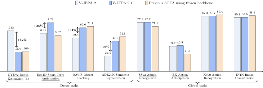
Recognizing a scene and locating every object inside it need different kinds of features. Earlier V-JEPA models can recognize actions well while producing patch features that are harder to use for depth or segmentation. V-JEPA 2.1 adds direct training targets for visible context tokens as well as masked tokens, and supervises several encoder layers. Together with native image/video tokenizers, broader data and larger models, this improves local spatial structure while retaining useful global recognition. The encoder stays frozen in the downstream studies, but task heads or action-conditioned world models are trained separately. Results cover perception and specific planning setups, rather than a single general-purpose autonomous agent.
1 Introduction
Dense tasks need each patch feature to retain its location and local content; global recognition can succeed with features that aggregate across the scene. The paper diagnoses this mismatch in V-JEPA 2 and modifies where prediction losses act. Deep supervision helps reconcile dense detail with high-level semantics, while data, model scaling and distillation complete the recipe. The main contribution is a more versatile representation, evaluated through distinct downstream systems.
2 Methodology
2.1 Preliminaries: Joint-Embedding Predictive Architectures
In the previous V-JEPA objective, an encoder sees visible tokens and a predictor estimates targets at masked positions. A momentum target encoder processes the full input. Constant representations would solve an unconstrained regression objective, so the tested recipe uses asymmetric updates and stop-gradient. The original loss directly supervises masked-token predictions only; visible context still receives indirect gradients through those predictions.
Equation 1
| (1) |
2.2 Analysis of V-JEPA Features for Dense Vision Tasks
Principal-component visualizations and frozen linear probes examine whether patch features preserve local structure. The diagnostic asks what is easily accessible from features, not whether a larger downstream model could recover additional information.
Observations and Hypothesis.
Earlier feature maps appear spatially fragmented and perform poorly on simple dense probes. The proposed explanation is that visible context tokens can act as global information aggregators because their own output locations lack a direct prediction target. This is an architectural hypothesis tested by a loss modification, not a theorem about every JEPA representation.
|
Image |
|
|
|
V-JEPA 2 |

|

|
|
|

|
|
Context Self-Supervision.
Adding a target-matching loss at visible context positions makes spatial structure more accessible and improves depth and segmentation probes. However, dense improvement alone does not preserve global recognition; subsequent components address that tradeoff.
Equation 2
| (2) |
2.3 V-JEPA 2.1: Improving Dense Video SSL Features
V-JEPA 2.1 combines a weighted loss across visible and masked tokens with supervision at multiple encoder depths. Modality-specific patch embeddings, broader data, larger encoders and smaller distilled models extend the resulting recipe.
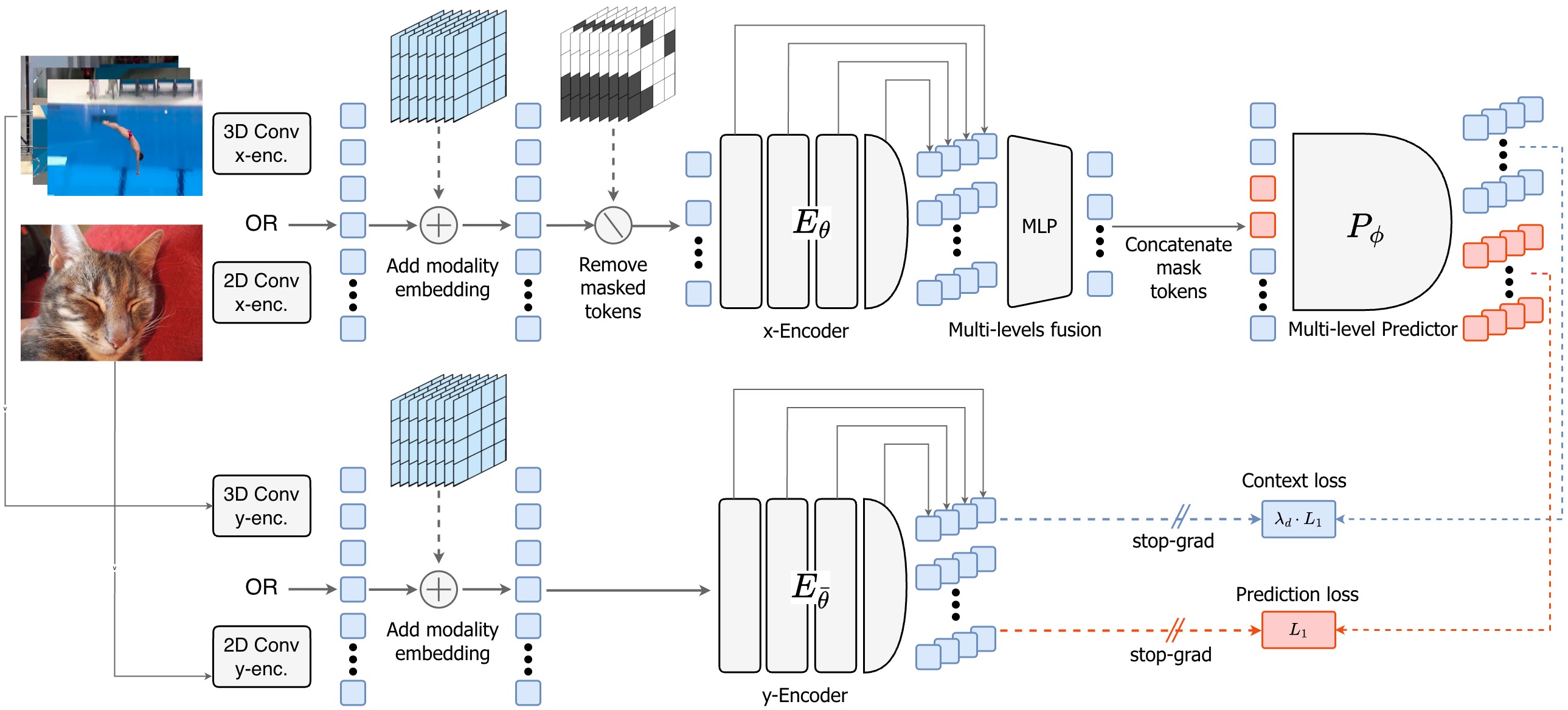
VJEPA 2.1 Architecture.
Image or video tokens enter a shared encoder. Features from several depths are fused, then combined with position-marked mask tokens for prediction. Masked and visible predictions are compared with corresponding full-input target features at several levels.
Implementation Details.
The main phase uses lower-resolution images and short videos. A brief cooldown increases image resolution and video duration/resolution while reducing learning rate. Component ablations use the first phase; final task results use the complete schedule.
Empirical Evaluation.
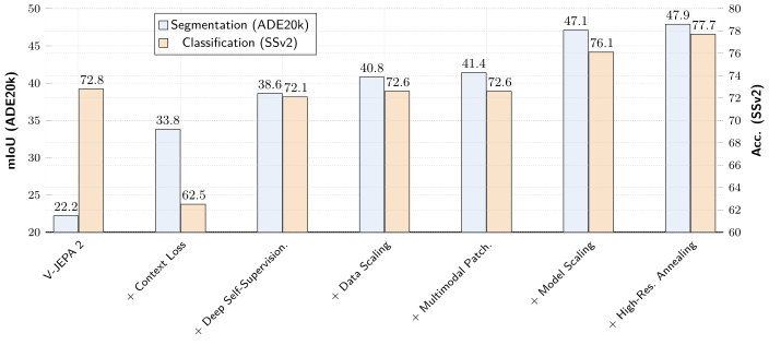
Dense linear probes test depth and segmentation, while attentive heads test object and action recognition. Using both reveals whether a change improves local features at the expense of global semantics.
| IN1K Acc. | SSv2 Acc. | NYU RMSE | ADE20K mIoU | |
| 82.2 | 72.8 | 0.682 | 22.2 | V-JEPA 2 |
| 72.6 | 62.5 | 0.474 | 33.8 | + Context Loss |
| 80.8 | 72.1 | 0.463 | 38.6 | + Multi-level Pred. |
| 81.6 | 72.6 | 0.418 | 40.8 | + Vision Mix |
| 81.6 | 72.6 | 0.415 | 41.4 | + Multi-modal Tok. |
| 84.8 | 76.1 | 0.365 | 47.1 | + Model Scaling |
| 85.5 | 77.7 | 0.307 | 47.9 | + Cool-down. |
| ADE20K mIoU | SSv2 Acc. | Scheme | Warmup | |
| 22.2 | 72.8 | V-JEPA 2, | cte | |
| 26.4 | 71.0 | 0.05 | cte | |
| 29.6 | 62.5 | 0.2 | cte | |
| 27.5 | 53.8 | 0.5 | cte | |
| 24.6 | 51.1 | 1.0 | cte | |
| 30.5 | 60.5 | 0.2 | cte | ✓ |
| 32.2 | 61.5 | 0.5 | cte | ✓ |
| 33.8 | 62.5 | 0.5 | weighted | ✓ |
2.3.1 Dense Prediction Loss
Uniformly matching visible features can encourage easy copying and damage global recognition. The method warms up the context loss and weights visible tokens more strongly near masked regions. This encourages continuity across the visible/hidden boundary.
The weighted context term improves the tested dense tasks but initially reduces recognition scores. The full recipe therefore depends on the following deep-supervision and scaling steps; context loss alone does not deliver every headline gain.
Equation 3
| (3) |
2.3.2 Deep Self-Supervision
The predictor receives fused features from several encoder depths and predicts targets at four levels. Applying both losses throughout the network improves local features while recovering global recognition. It also makes final-layer features more useful, reducing dependence on extracting several layers at evaluation.
2.3.3 Scaling Image Data.
A 142 million-image collection expands appearance coverage, while video sampling emphasizes motion-rich and heterogeneous clips. Image-only and video-only workers contribute gradients to the shared model. The tested batch mixture and curated data distribution are important ingredients, beyond the loss modification.
| Source | Samples | Type | Total Hours | V-JEPA2 weights | V-JEPA2.1 weights |
| SSv2 (Goyal et al., 2017) | 168K | EgoVideo | 168 | 0.056 | 0.170 |
| Kinetics (Carreira et al., 2019) | 733K | ExoVideo | 614 | 0.188 | 0.010 |
| Howto100M (Miech et al., 2019) | 1.1M | ExoVideo | 134K | 0.318 | 0.100 |
| ImageNet (Deng et al., 2009) | 1M | Images | n/a | 0.250 | 0. |
| YT-1B (Zellers et al., 2022) | 19M | ExoVideo | 1.6M | 0.188 | 0.720 |
| LVD-142M (Oquab et al., 2023) | 142 M | Curated images | n/a | ||
2.3.4 Multi-Modal Tokenizer
A two-dimensional image patchifier and a three-dimensional video patchifier feed the same encoder. Learned modality tokens identify the input type. Images can now be processed directly rather than copied into artificial still videos, saving computation and avoiding that formatting bias.
2.3.5 Scaling Model Size to ViT-G (2B) and High-Resolution Cool-Down
Scaling from 300 million to two billion encoder parameters improves the selected dense and global tests. A higher-resolution cooldown further improves them, especially depth. Capacity, resolution and schedule all contribute to the strongest final model.
2.3.6 Model Distillation
A frozen large teacher supplies final-layer targets to smaller students. Distillation omits deep supervision and uses a new smaller predictor; an averaged student is released for evaluation. Distilled small-model performance therefore includes knowledge transferred from the large teacher.
3 Results
All downstream experiments freeze the visual encoder. Some train supervised probes, others train additional action-conditioned or language-aligned systems. Their results test different uses of the representation, rather than a single unchanged inference pipeline.
3.1 Short-Term Object Interaction Anticipation
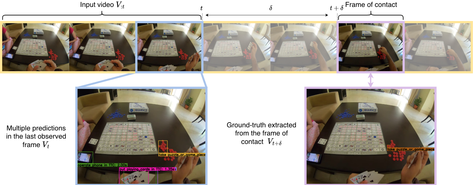
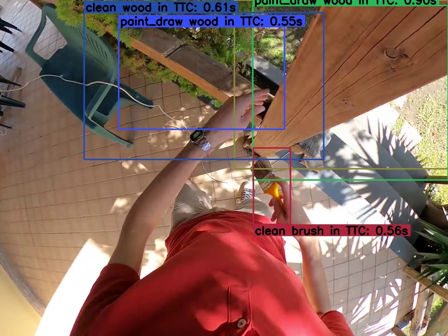
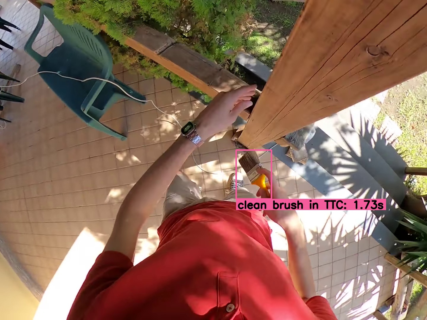
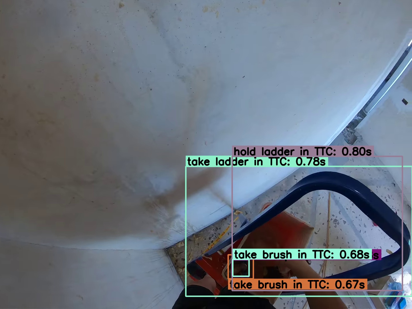
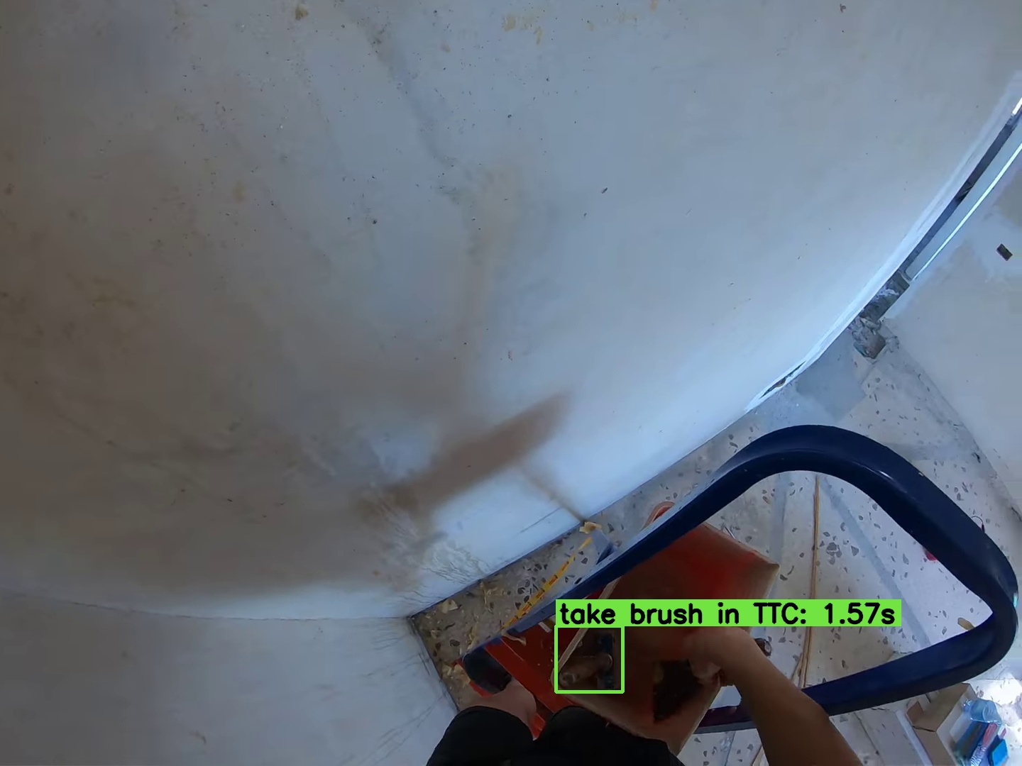
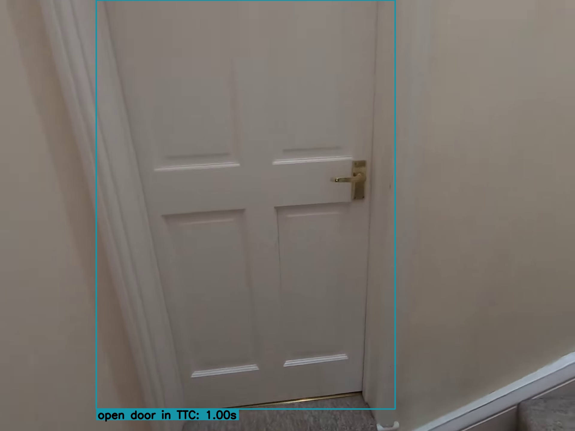
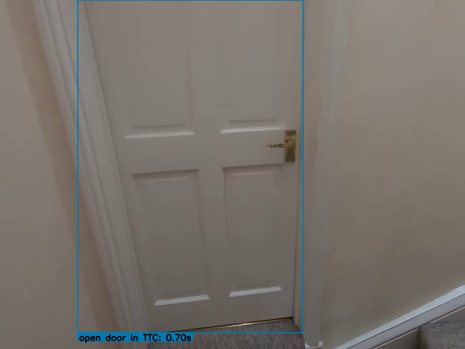
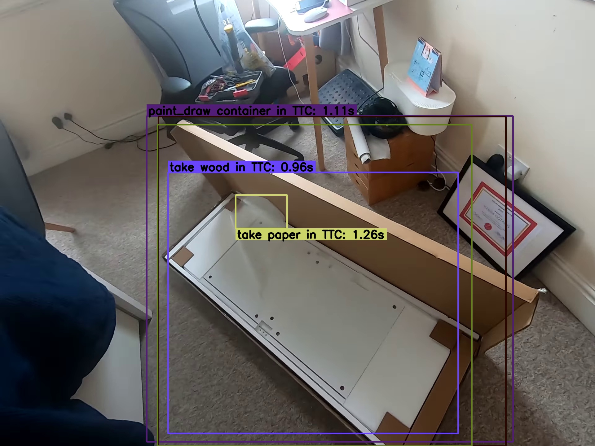
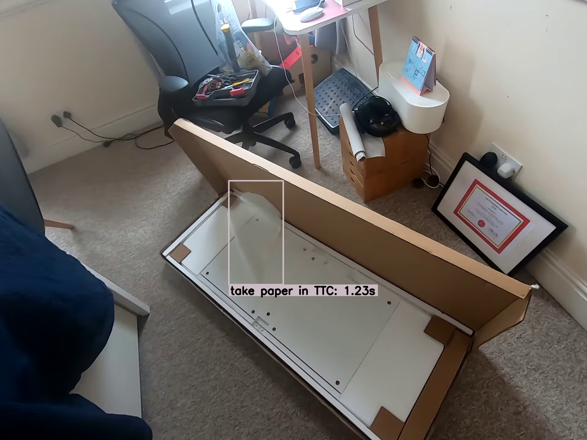
Short-term anticipation predicts which object a person will interact with, its image location, the action and time until contact. This jointly tests local detail and temporal context.
| Model | AP b | AP b+N | AP b+V | AP b+ | AP b+N+V | AP b++N | AP b++V | AP All | mAP N | mAP N+V | mAP N+ | mAP All |
| Results Reported in the Literature | ||||||||||||
| StillFast (Ragusa et al., 2023) | - | - | - | - | - | - | - | - | 20.2 | 10.3 | 7.17 | 3.96 |
| STAformer (Mur-Labadia et al., 2024) | 38.3 | 28.3 | 16.6 | 12.27 | 12.8 | 8.89 | 5.47 | 4.06 | 29.4 | 15.3 | 9.94 | 5.67 |
| GANO (Thakur et al., 2023) | 45.3 | 27.0 | 12.2 | 16.6 | 6.54 | 9.0 | 4.18 | 2.47 | - | - | - | - |
| Encoders using our same protocol | ||||||||||||
| DINOv2 ViT-L (Oquab et al., 2023) | 45.1 | 37.8 | 21.9 | 14.4 | 17.6 | 10.6 | 7.27 | 5.25 | 28.3 | 15.2 | 9.22 | 5.25 |
| DINOv2 ViT-g (Oquab et al., 2023) | 47.8 | 38.1 | 23.6 | 14.1 | 19.1 | 10.9 | 7.29 | 5.73 | 30.6 | 16.8 | 9.37 | 5.44 |
| DINOv3 ViT-H+ (Siméoni et al., 2025) | 48.9 | 40.2 | 23.4 | 13.6 | 19.4 | 10.8 | 6.71 | 5.45 | 32.4 | 17.2 | 9.53 | 5.20 |
| DINOv3 ViT-7B (Siméoni et al., 2025) | 50.2 | 40.9 | 23.8 | 14.2 | 19.8 | 11.5 | 7.33 | 5.82 | 33.8 | 17.4 | 10.3 | 5.68 |
| V-JEPA 2 ViT-g (Assran et al., 2025) | 45.7 | 34.4 | 22.2 | 16.7 | 16.9 | 12.1 | 8.56 | 6.26 | 27.2 | 14.9 | 10.4 | 6.02 |
| V-JEPA 2.1 ViT-g | 47.3 | 36.5 | 23.6 | 18.1 | 18.2 | 13.5 | 9.55 | 7.21 | 28.7 | 15.5 | 11.4 | 6.75 |
| V-JEPA 2.1 ViT-G | 50.7 | 39.3 | 25.8 | 20.2 | 20.3 | 15.1 | 10.8 | 8.20 | 30.9 | 17.2 | 12.8 | 7.71 |
Task.
Ego 4D’s strict combined metric requires an overlapping box, correct noun and verb, and a sufficiently accurate contact time. Its top-five convention accommodates several possible futures. A 7.71 mAP score is this specialized detection/anticipation metric, not 7.71% overall action accuracy.
| V-JEPA 2.1 Prediction | Ground-truth | V-JEPA 2.1 Prediction | Ground-truth |
 |
 |
 |
 |
 |
 |
 |
 |
Evaluation protocol.
Frozen video features are combined with features from a high-resolution last-frame image. A trained attentive pooling module and extended Faster R-CNN head produce localized interaction predictions. The result depends on that supervised detection pipeline as well as the encoder.
Results.
The reported combined anticipation score improves over the selected prior systems. Component metrics show gains in localization, action and timing. Qualitative examples illustrate plausible predictions; ambiguity and the benchmark’s matching rules remain part of the interpretation.
3.2 Action Anticipation
EPIC-KITCHENS action anticipation evaluates a fixed verb–noun vocabulary one second before an action, separately from localized Ego 4D interaction prediction.
Task.
The kitchen benchmark has predefined action categories and annotated time segments. Mean-class recall at five measures whether the true label appears among five guesses, not whether the model identifies an arbitrary future action.
Evaluation protocol.
A supervised attentive head combines observed encoder features and predicted future features. Separate classifier queries predict nouns, verbs and complete actions; focal loss addresses the imbalanced categories.
| Method | Param. | Action Anticipation | ||
| Verb | Noun | Action | ||
| InAViT (Roy et al., 2024) | 160M | 51.9 | 52.0 | 25.8 |
| Video-LLaMA (Zhang et al., 2023) | 7B | 52.9 | 52.0 | 26.0 |
| PlausiVL (Mittal et al., 2024) | 8B | 55.6 | 54.2 | 27.6 |
| V-JEPA 2 ViT-g (Assran et al., 2025) | 1B | 63.6 | 57.1 | 39.7 |
| V-JEPA 2.1 ViT-g | 1B | 63.6 | 56.2 | 38.4 |
| V-JEPA 2.1 ViT-G | 2B | 64.3 | 59.9 | 40.8 |
Results.
At the same one-billion-parameter scale, V-JEPA 2.1 is comparable to V-JEPA 2 on this task. The larger two-billion-parameter model reaches 40.8 action recall at five. The improvement therefore includes model scaling rather than isolating the dense loss.
3.3 Robotic Arm Planning
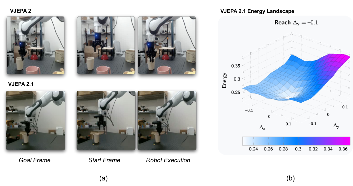
A separate action-conditioned predictor is trained on DROID recordings above frozen V-JEPA 2.1 features, following the earlier robot-control setup. Goal-image planning is evaluated on reaching, grasping and pick-and-place.
The reported grasping outcome improves, and an eight-step rollout with a changed sampling budget helps further; the earlier representation degrades with that longer horizon. Failures still include closing or opening the gripper at the wrong time. These experiments support improved local geometry within this specific controller, not unrestricted manipulation or automatic long-horizon task decomposition.
| Planning Details | |||||||
| Method | #Samples | Iter. | Horizon | Time | Reach | Grasp | Pick-&-Place |
| VJEPA 2 (Assran et al., 2025) | 800 | 10 | 1 | 3 sec. | 100% | 60% | 80% |
| VJEPA 2.1 (ours) | 800 | 10 | 1 | 3 sec. | 100% | 70% | 80% |
| 300 | 15 | 8 | 14 sec. | 100% | 80% | 80% | |
3.4 Navigation Planning
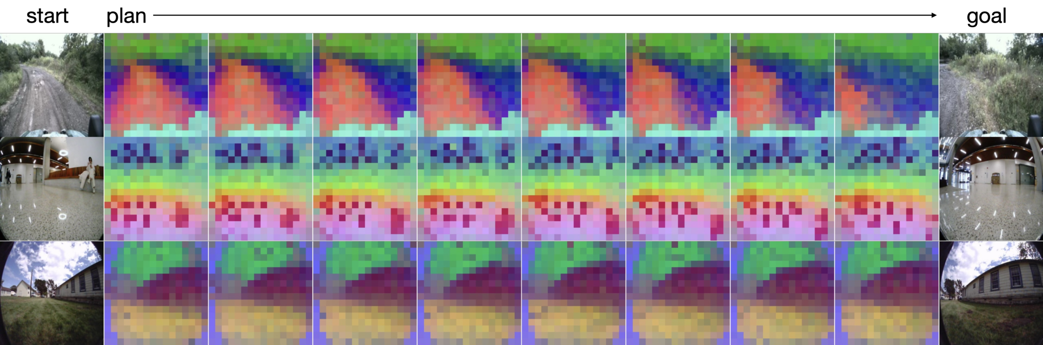
The navigation study plans two-second candidate trajectories toward an image goal using a separately trained latent diffusion world model. It predicts clean representations and uses a less stochastic sampler to manage high-dimensional features. A reduced three-degree-of-freedom action space limits the search.
The tested system needs fewer denoising steps and achieves lower trajectory errors with faster planning than the compared latent baseline. Those speed and accuracy results belong to this specific world-model and sampling setup, not to the encoder alone.
| Model | Time | Recon | Tartan Drive | Scand | Sacson | Average | |||||
| ATE | RTE | ATE | RTE | ATE | RTE | ATE | RTE | ATE | RTE | ||
| NWM (Bar et al., 2025) | (s) | 1.146 | 0.339 | 5.831 | 1.219 | 1.113 | 0.297 | 4.037 | 0.928 | 3.032 | 0.696 |
| V-JEPA 2.1 ViT-g | 10.6 (s) | 1.146 | 0.338 | 5.758 | 1.200 | 1.094 | 0.299 | 3.904 | 0.921 | 2.975 | 0.690 |
| V-JEPA 2.1 ViT-G | 10.6 (s) | 1.179 | 0.340 | 5.687 | 1.187 | 1.038 | 0.285 | 4.054 | 0.938 | 2.990 | 0.688 |
| Method | Param. | Depth | Segmentation | VOS | ||||
| NYUv2 | KITTI | ADE20k | Citysc. | VOC | DAVIS-S | YT VOS-S | ||
| 7B models | ||||||||
| Web-DINO (Fan et al., 2025) | 7B/14 | 0.466 | 3.158 | 42.7 | 68.3 | 76.1 | 57.2 | 43.9 |
| DINOv3 (Siméoni et al., 2025) | 7B/16 | 0.309 | 2.346 | 55.9 | 81.1 | 86.6 | 71.1 | 74.1 |
| Models less than 2B parameters | ||||||||
| PEcore (Bolya et al., 2025) | 2B/14 | 0.590 | 4.119 | 38.9 | 61.1 | 69.2 | 48.2 | 34.7 |
| PEspatial (Bolya et al., 2025) | 2B/14 | 0.362 | 3.082 | 49.3 | 73.2 | 82.7 | 68.4 | 68.5 |
| AM-RADIOv2.5 (Ranzinger et al., 2024) | 1B/14 | 0.340 | 2.918 | 53.0 | 78.4 | 85.4 | 66.5 | 70.1 |
| InternVideo2-1B (Wang et al., 2024b) | 1B/14 | 0.471 | 4.739 | 28.4 | 35.6 | 65.2 | 50.6 | 51.2 |
| SigLIP 2 (Tschannen et al., 2025) | 1B/16 | 0.494 | 3.273 | 42.7 | 64.8 | 72.7 | 56.1 | 52.0 |
| DINOv2 (Oquab et al., 2023) | 1B/14 | 0.372 | 2.624 | 49.5 | 75.6 | 83.1 | 63.9 | 65.6 |
| DINOv3 ViT-H+ (Siméoni et al., 2025) | 0.8B/16 | 0.352 | 2.635 | 54.8 | 79.5 | 85.8 | 71.1 | 74.0 |
| V-JEPA2 ViT-g (Assran et al., 2025) | 1B/16 | 0.642 | 4.650 | 24.4 | 45.9 | 63.9 | 52.5 | 53.7 |
| V-JEPA 2.1 ViT-g | 1B/16 | 0.350 | 2.601 | 47.8 | 71.8 | 84.7 | 68.1 | 72.3 |
| V-JEPA 2.1 ViT-G | 2B/16 | 0.307 | 2.461 | 47.9 | 73.5 | 85.0 | 69.0 | 72.7 |
| NYUv2 | KITTI | |||
| Image | 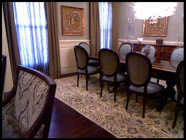 |
 |
 |
 |
| V-JEPA 2 | 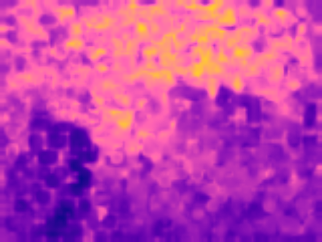 |
 |
 |
 |
|
V-JEPA 2.1 |
 |
 |
 |
 |
| Image | Ground-truth | DINOv3 | V-JEPA 2 | V-JEPA 2.1 |
|
|
|
|
|
|
|
|
|
|
|
|
|
|
|
|
|
|
|
|
|
|
|
|
|
3.5 Depth Estimation and Semantic Segmentation
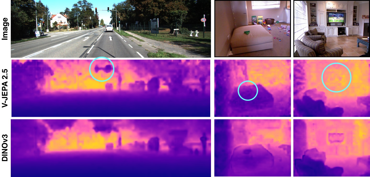
Depth and segmentation directly test whether frozen patch features preserve scene geometry and semantic boundaries.
Task.
Depth uses NYUv 2 and KITTI with root-mean-square error, where lower is better. Segmentation uses VOC12, ADE20K and Cityscapes with mean intersection over union, where higher is better.
Evaluation protocol.
A dense linear projection is trained above frozen final-layer image features. The protocol avoids intermediate encoder layers for these comparisons, making improved final-layer locality central to the result.
Results.
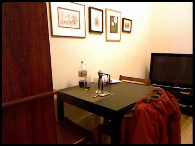
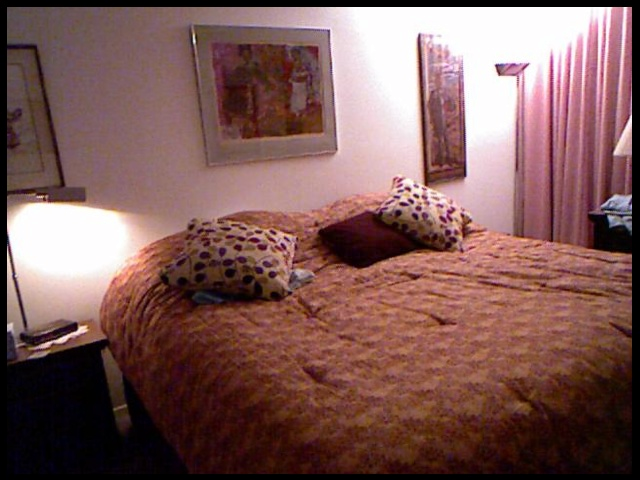
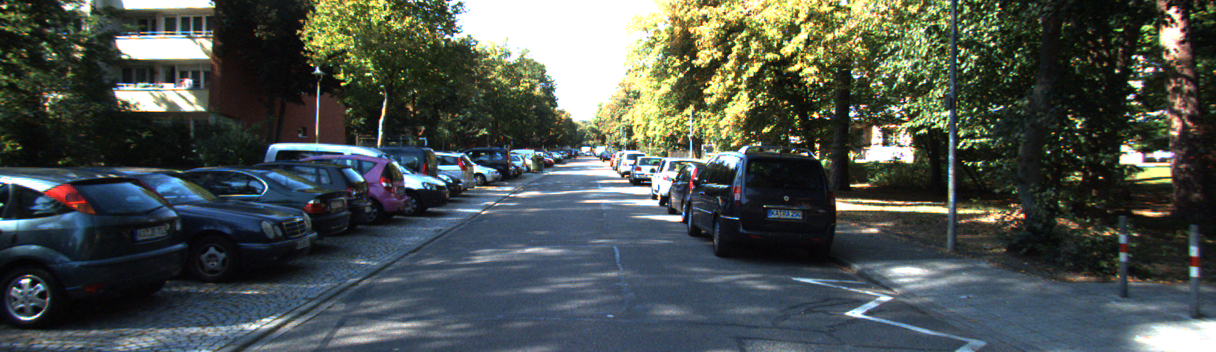
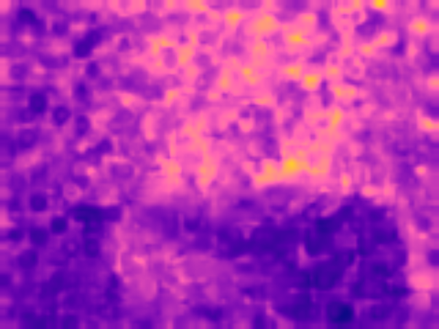
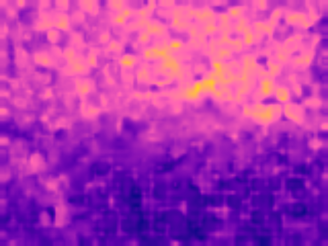
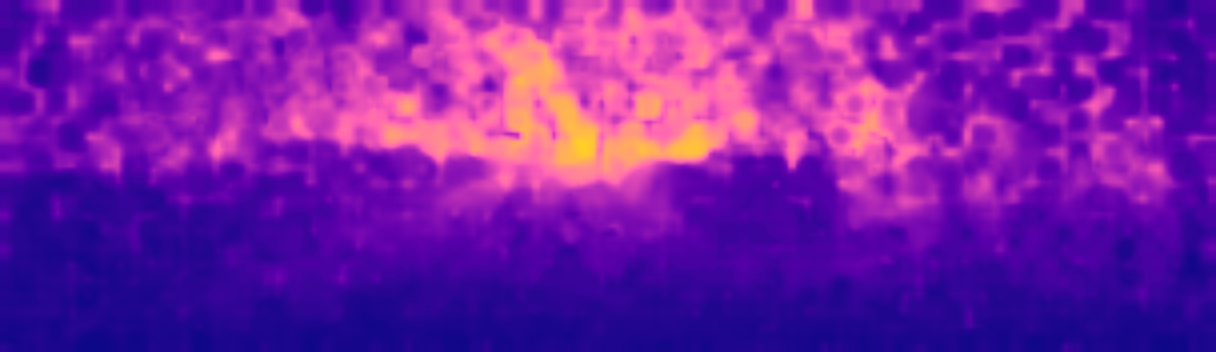
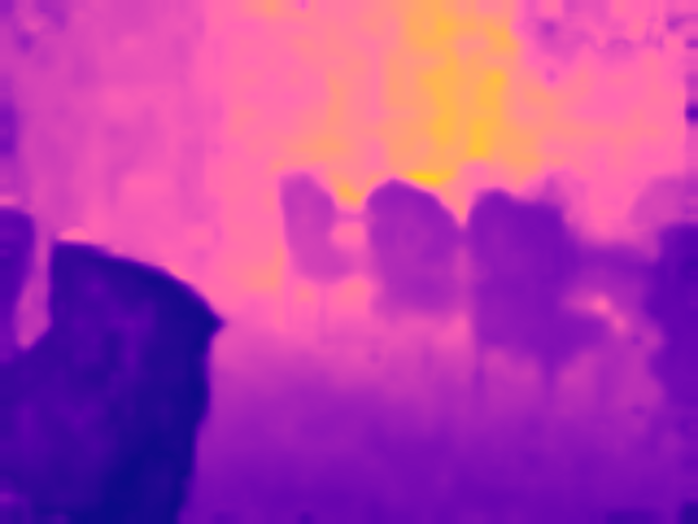
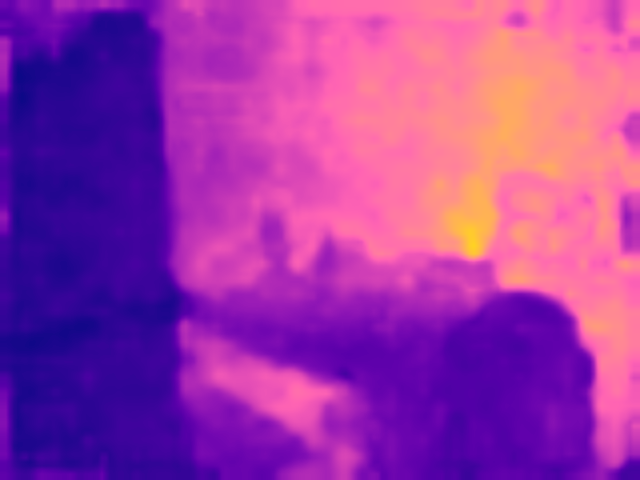
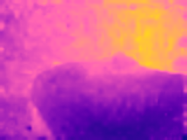
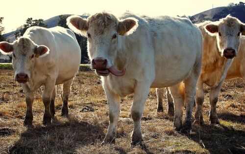
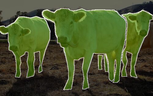
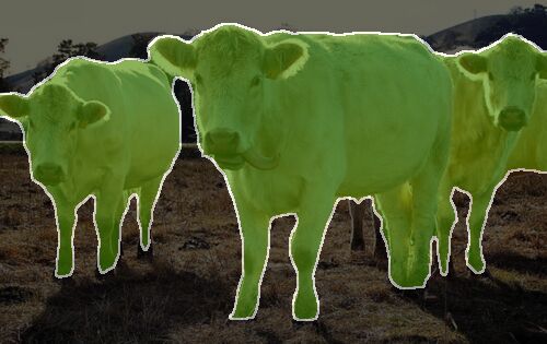
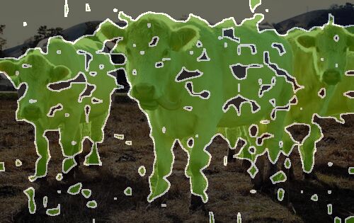
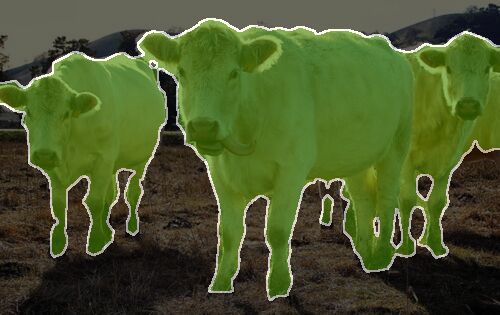
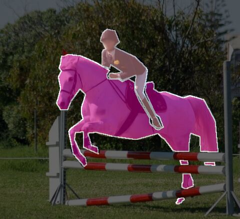
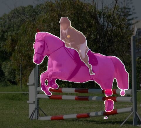
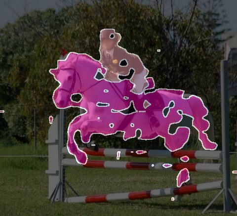
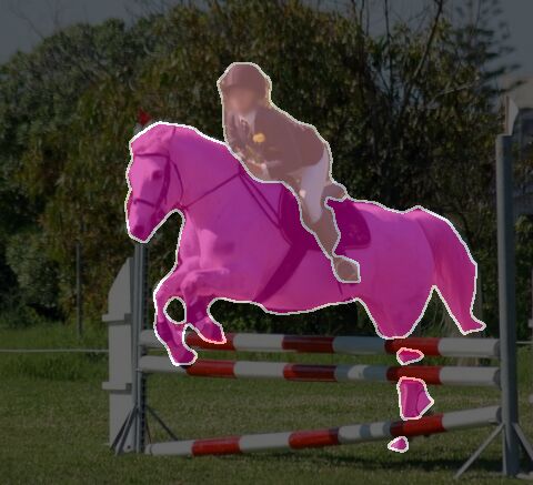
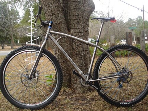
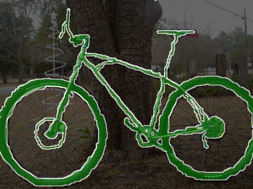
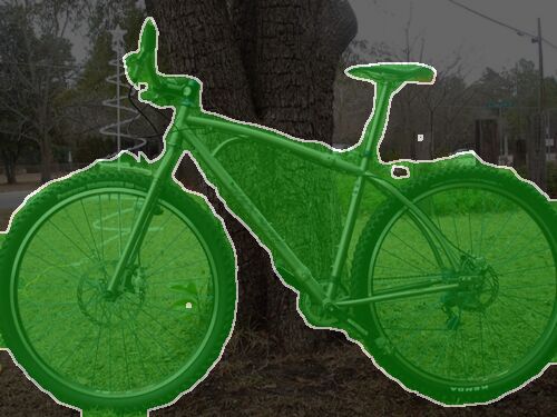
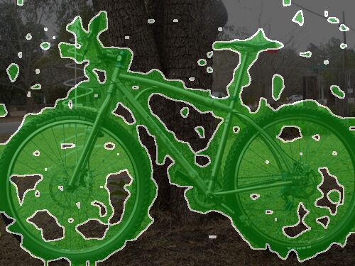
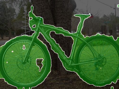
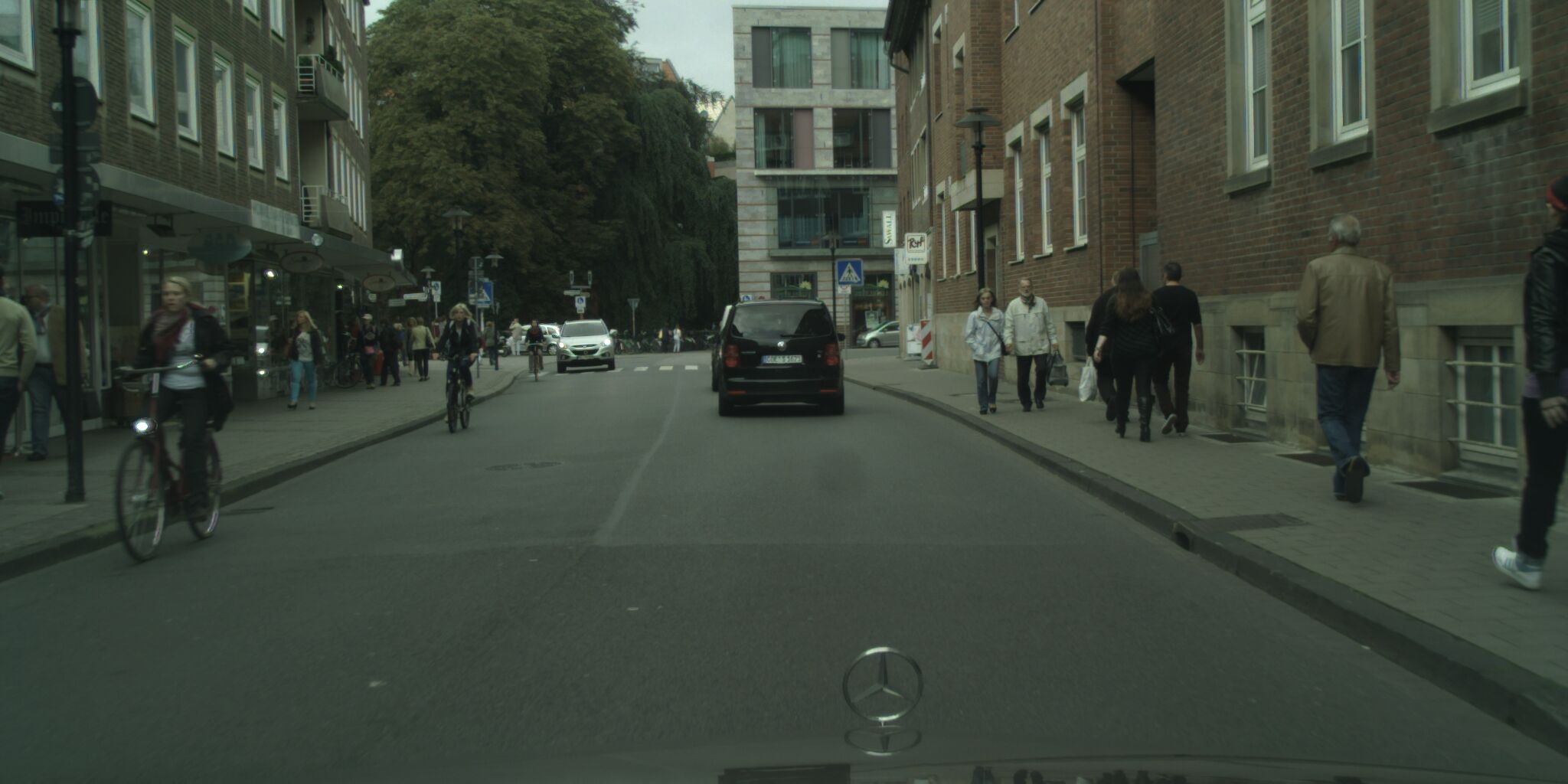
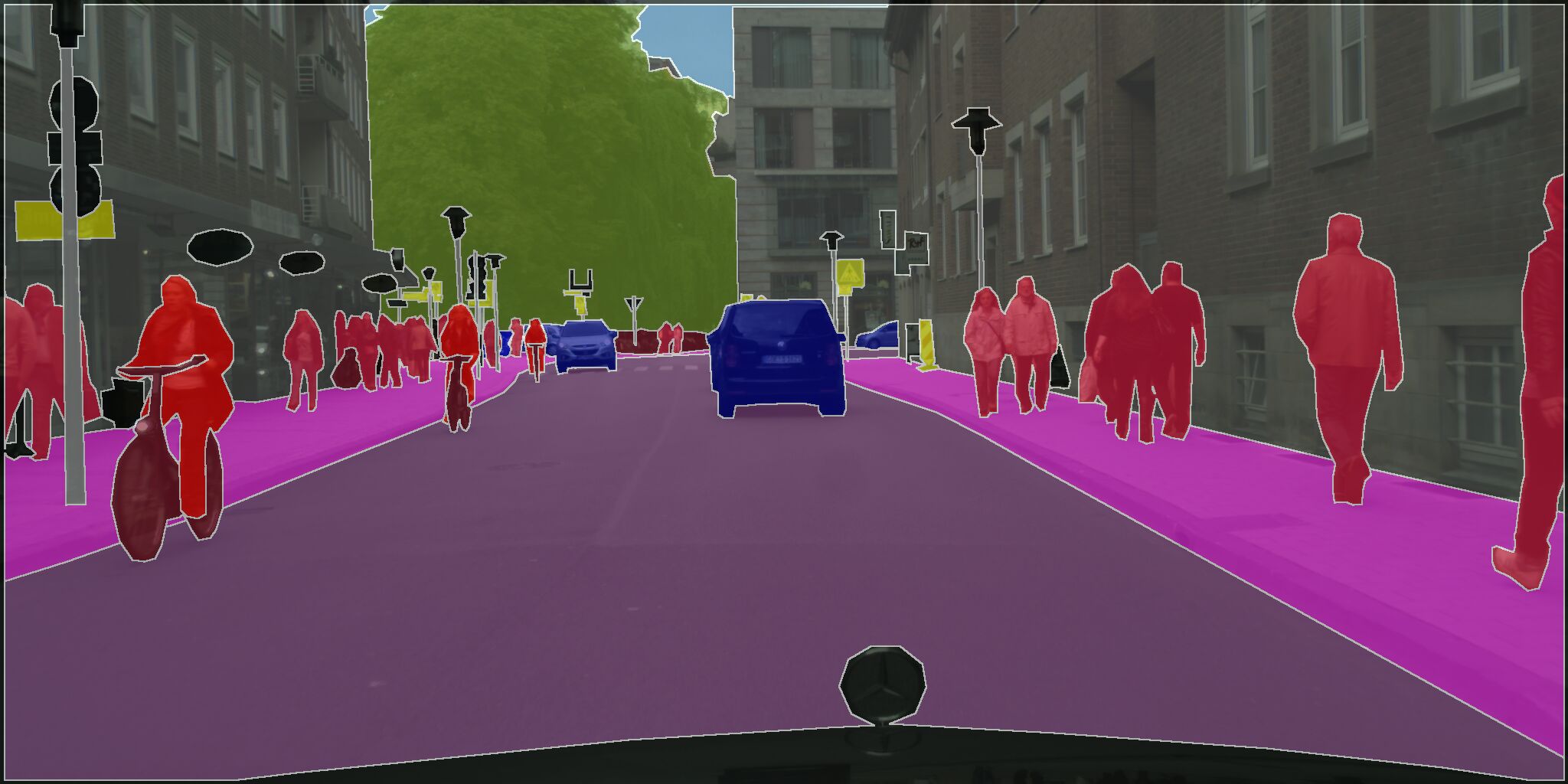
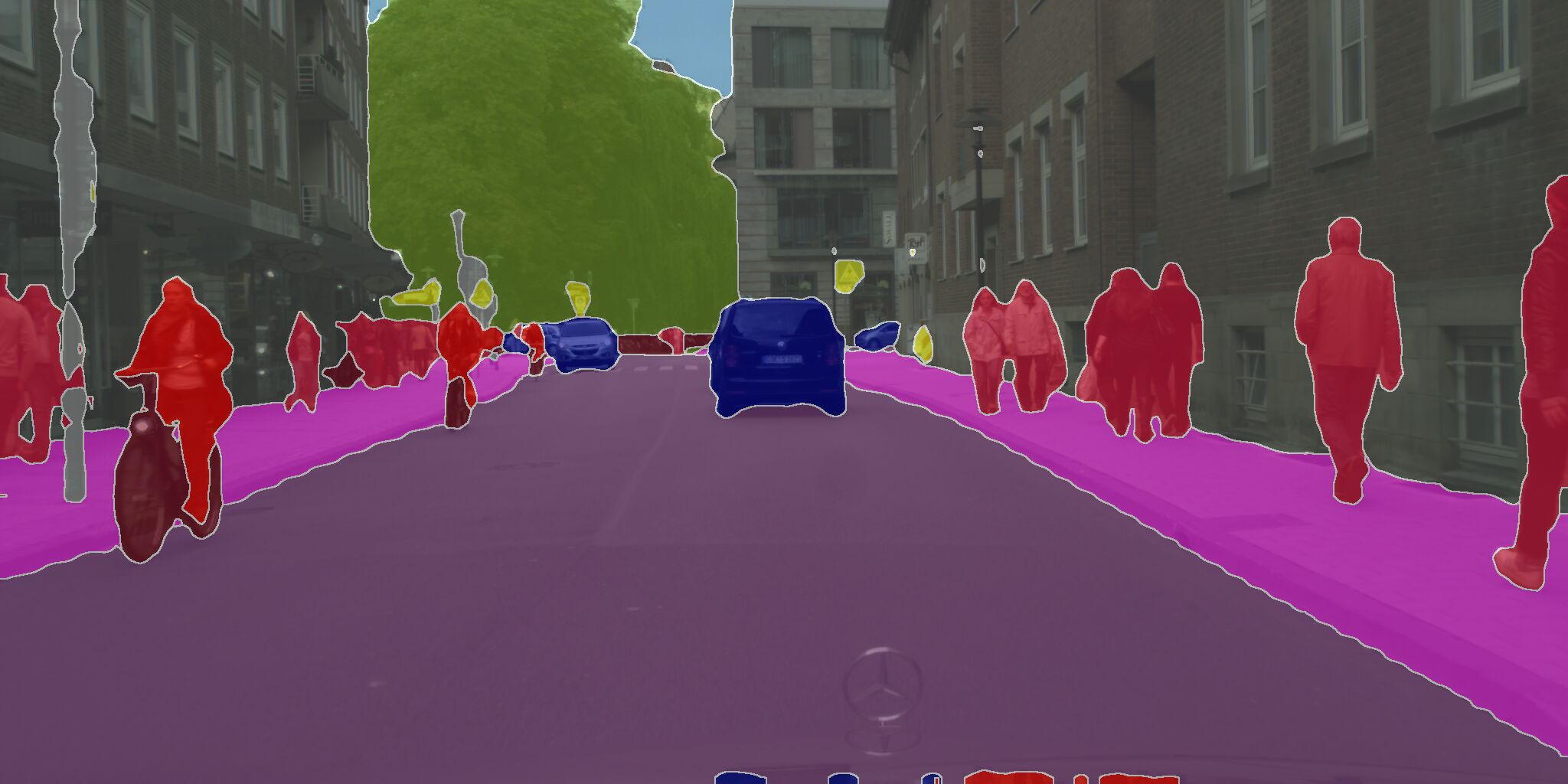
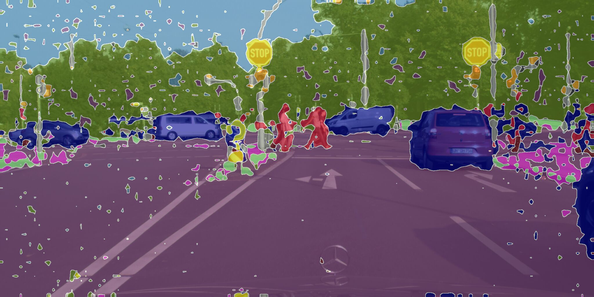
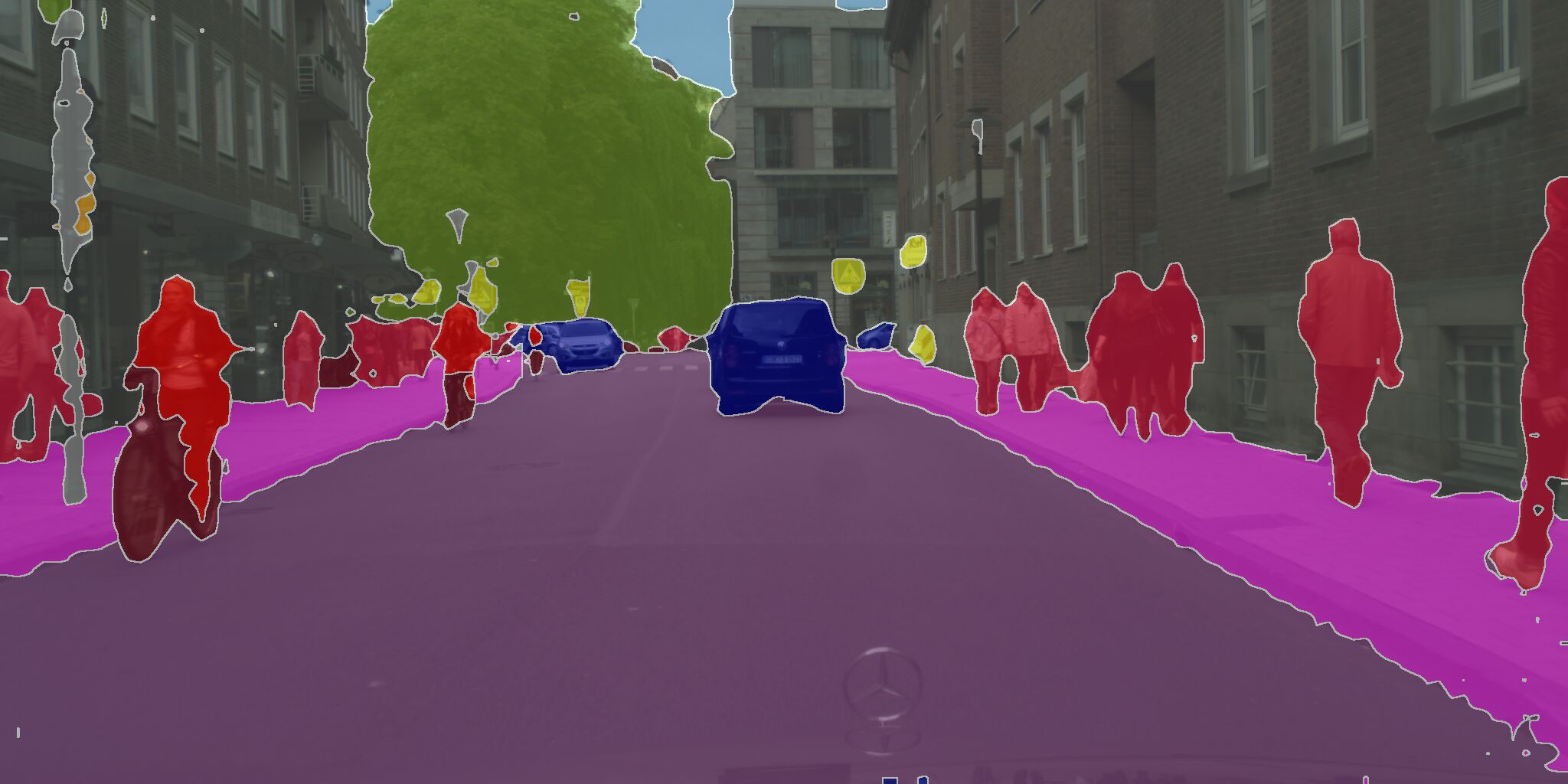
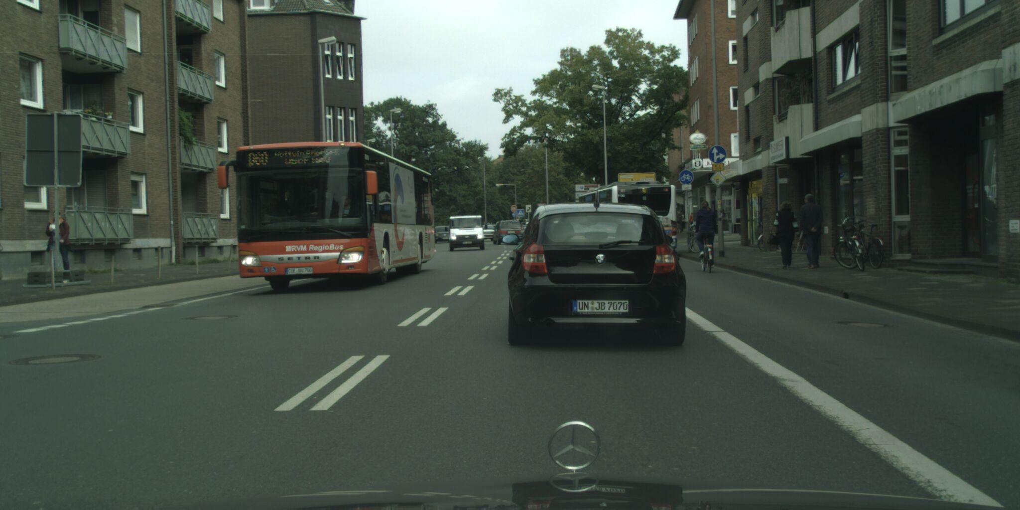
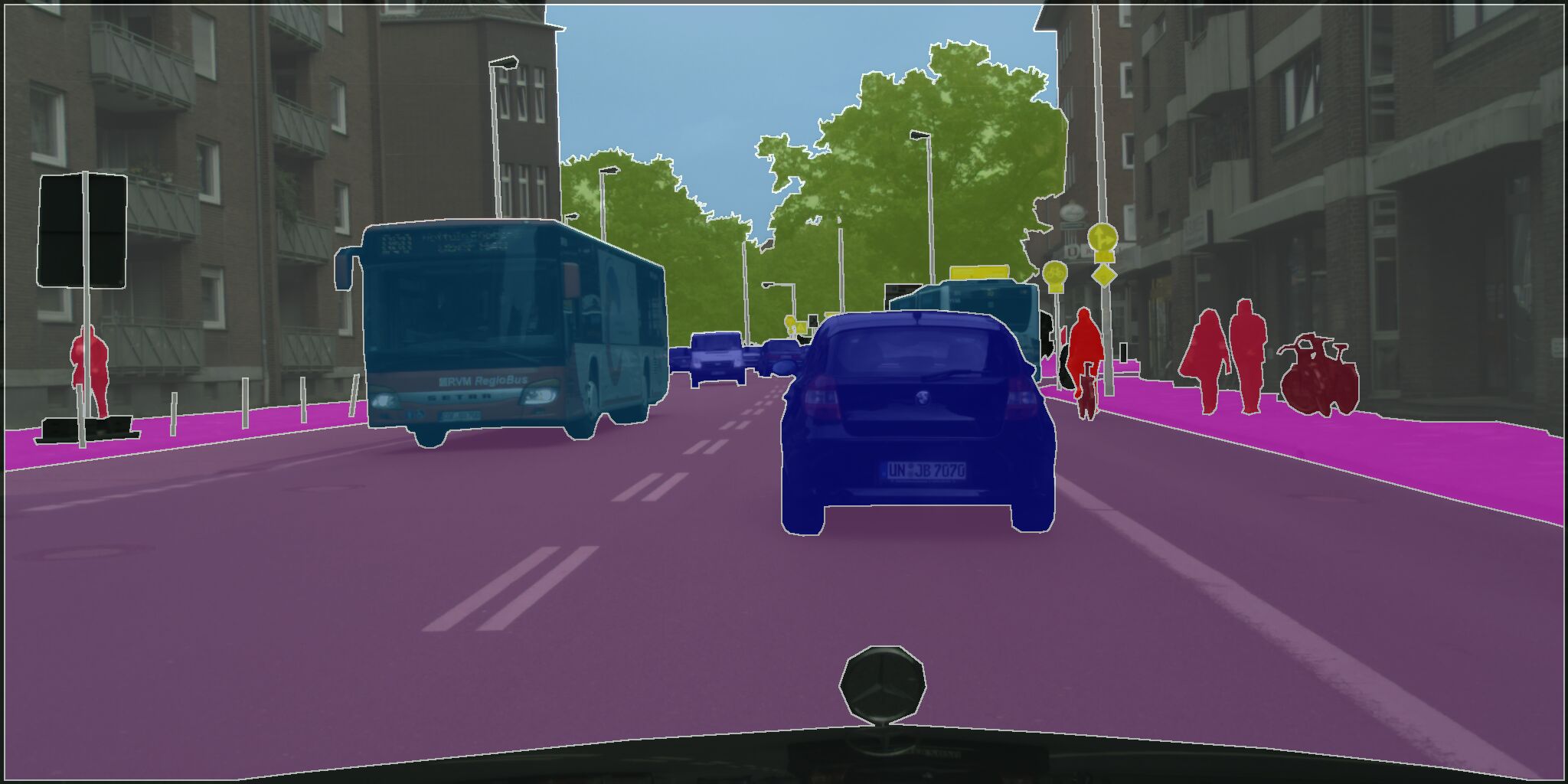
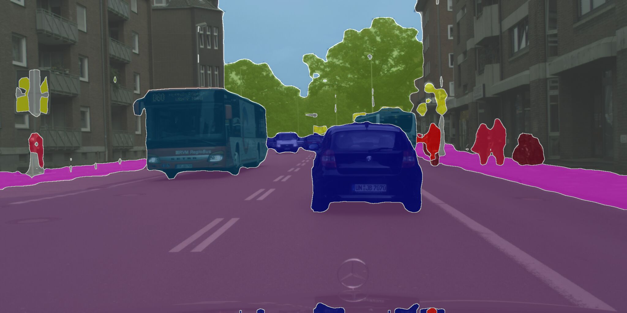
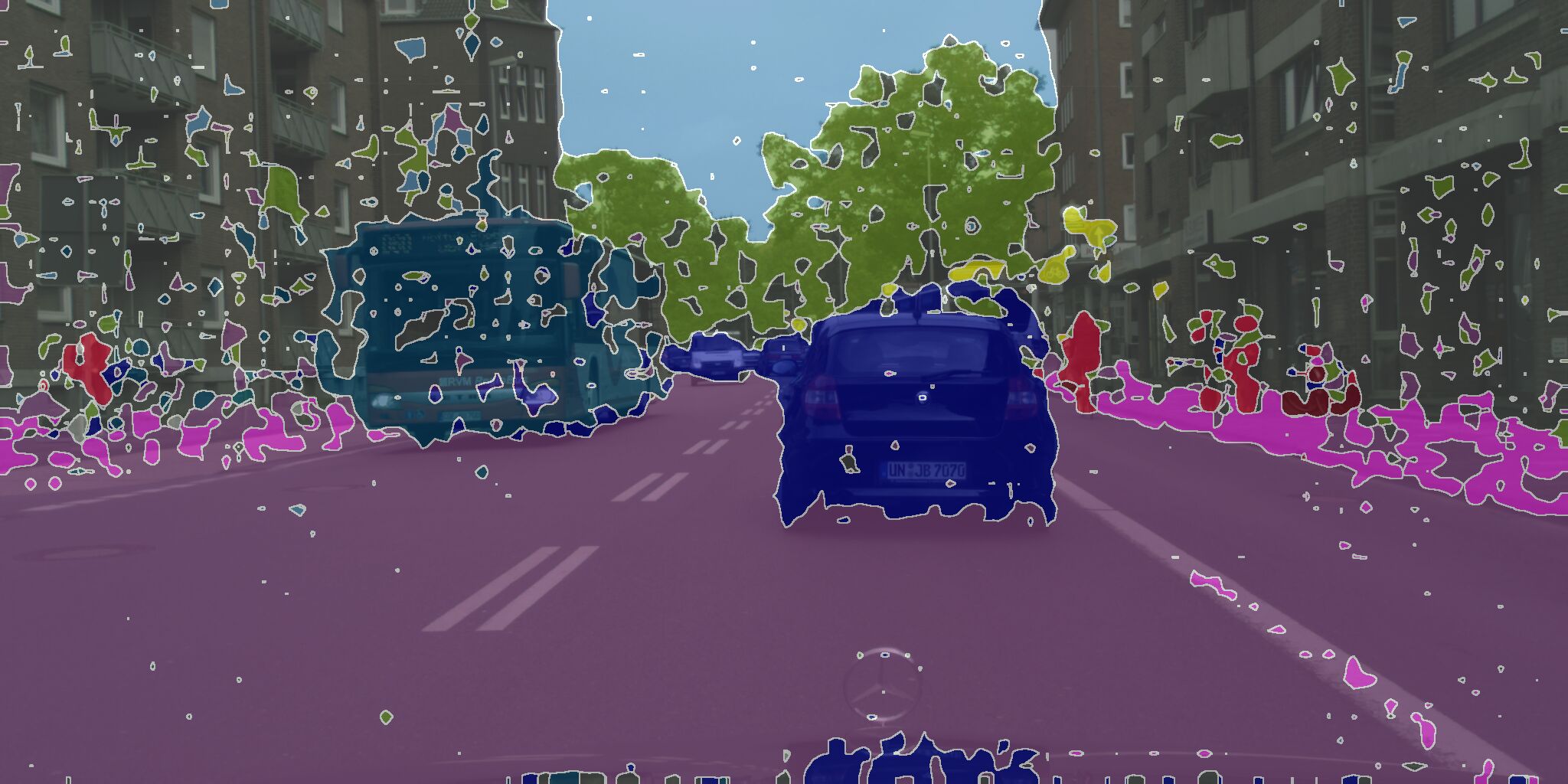
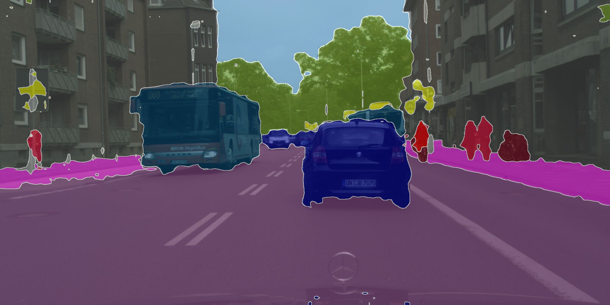
The largest model strongly improves dense probes over V-JEPA 2. It is especially competitive on depth, while some image encoders remain stronger on ADE20K or Cityscapes segmentation. Qualitative maps show sharper boundaries; the data-composition explanation for remaining gaps is a hypothesis.
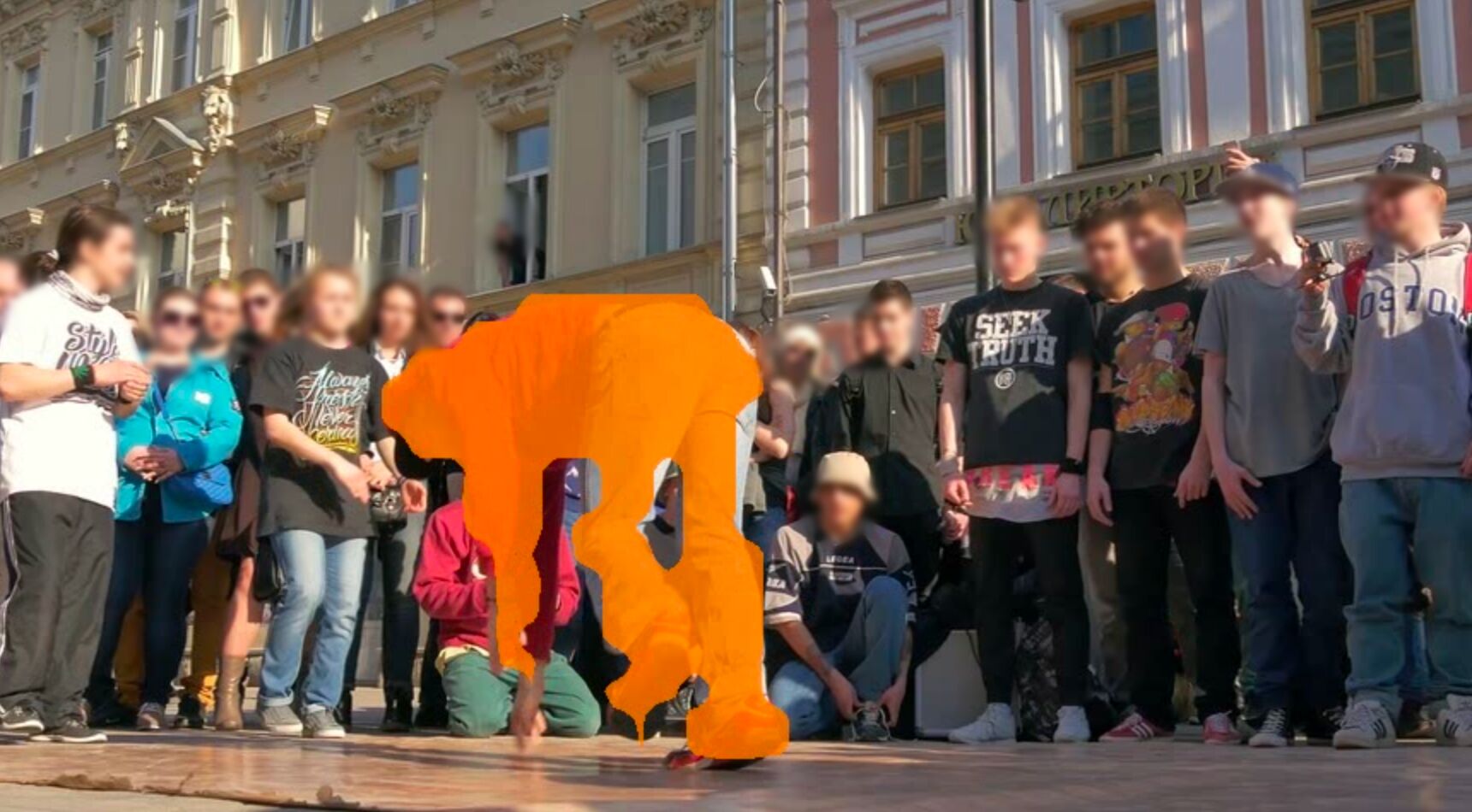
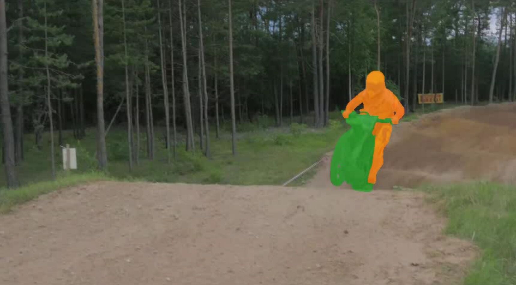
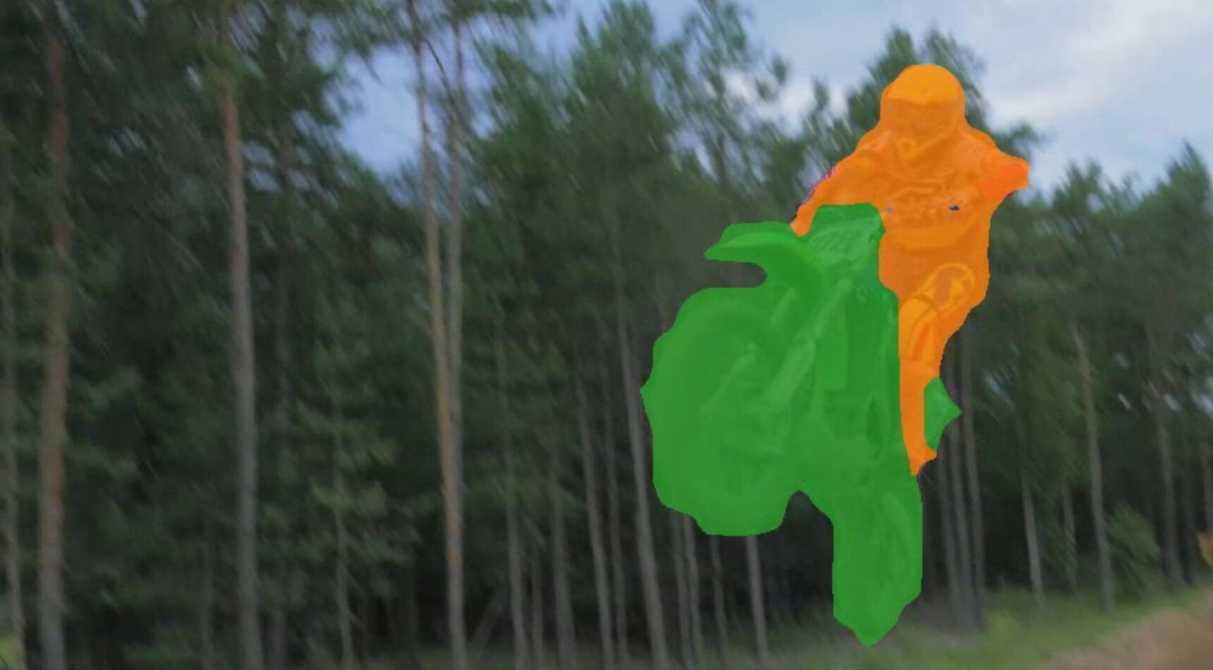
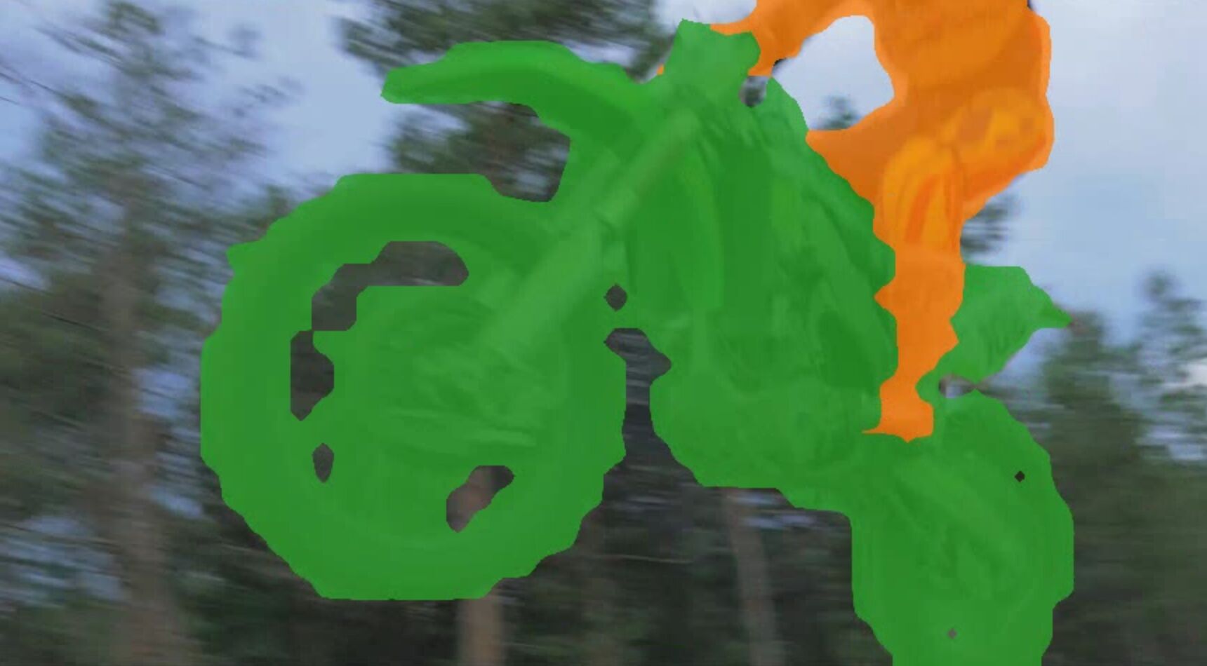
3.6 Video Object Segmentation
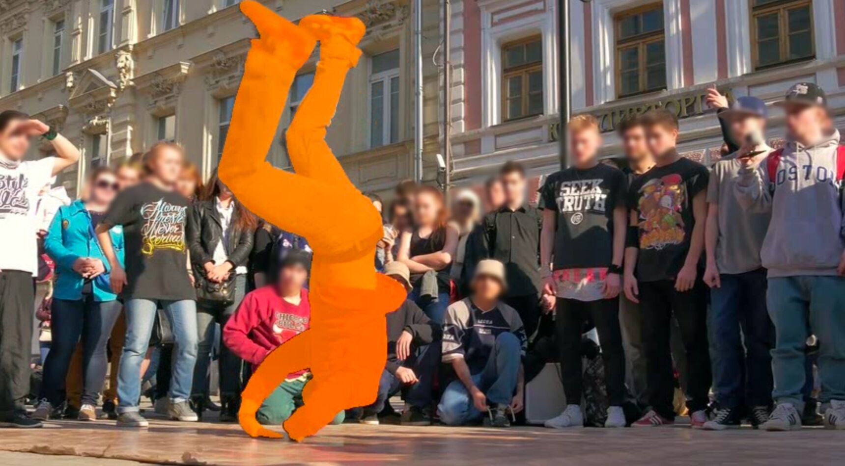
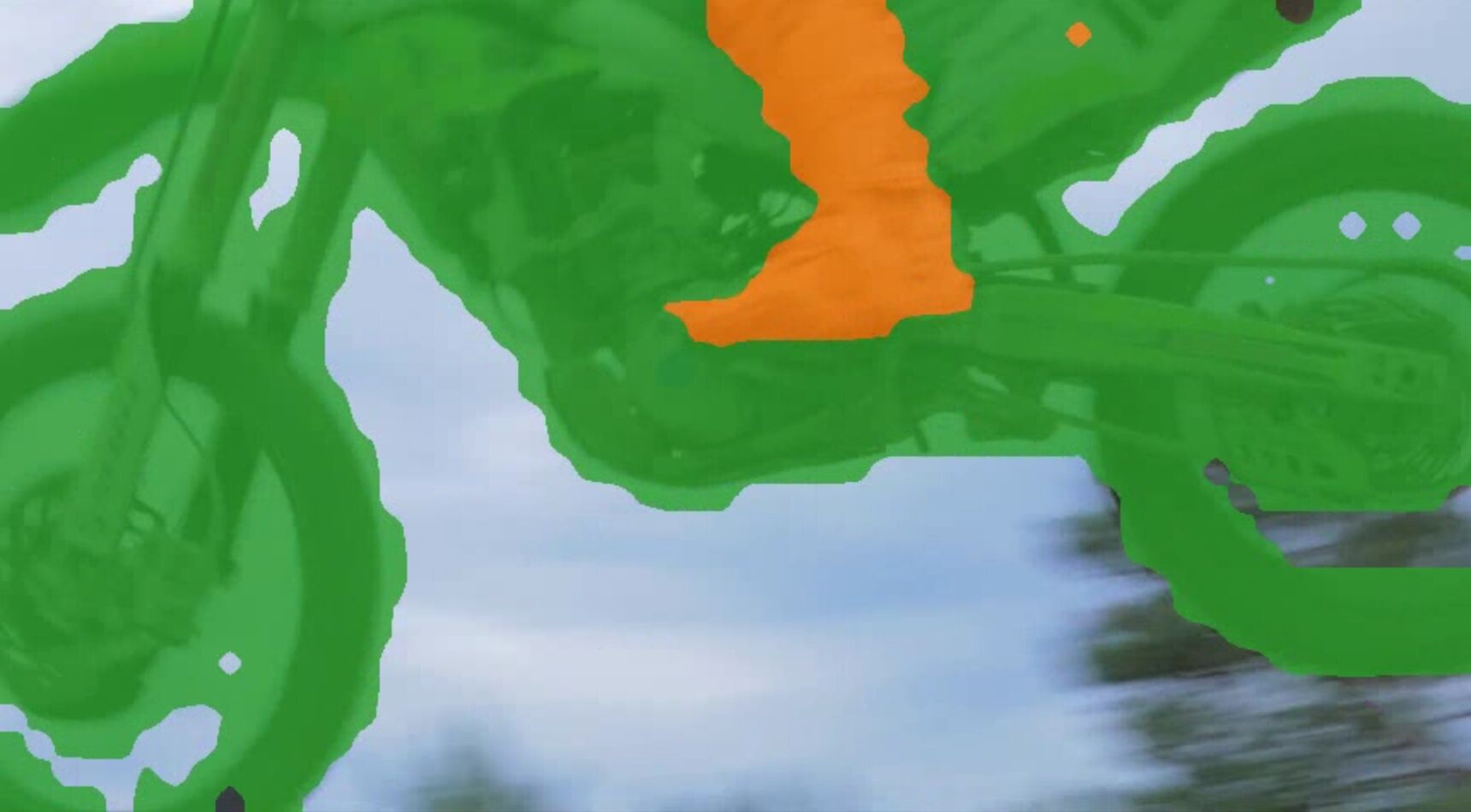
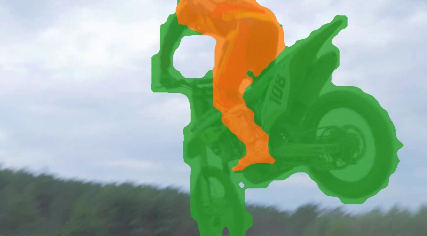
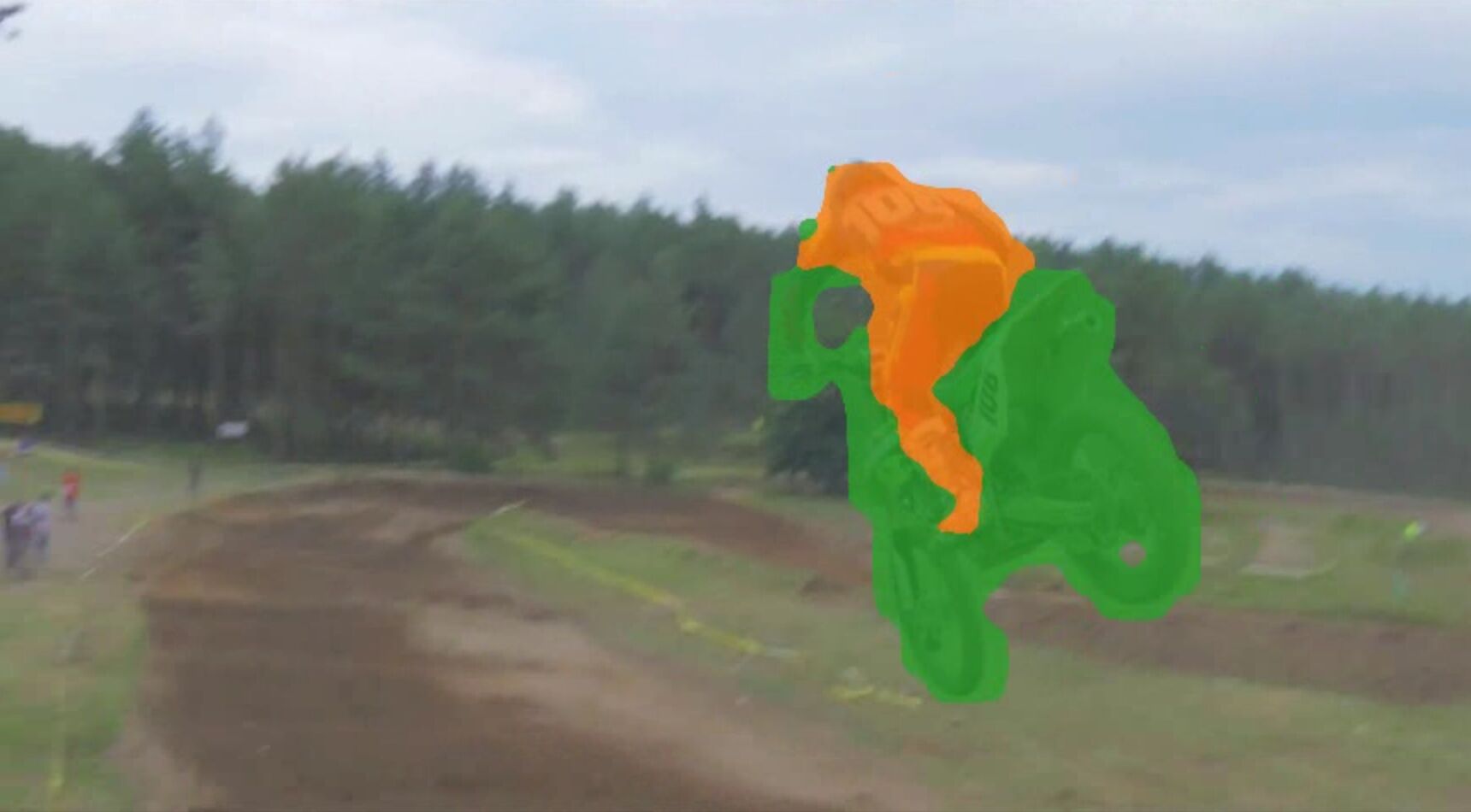
Video-object segmentation examines whether patch features stay comparable as an object moves or changes appearance.
| Initial GT frame | Frames sequence | ||||
|
|
|
|
|
|
|
|
|
|
|
|
Task.
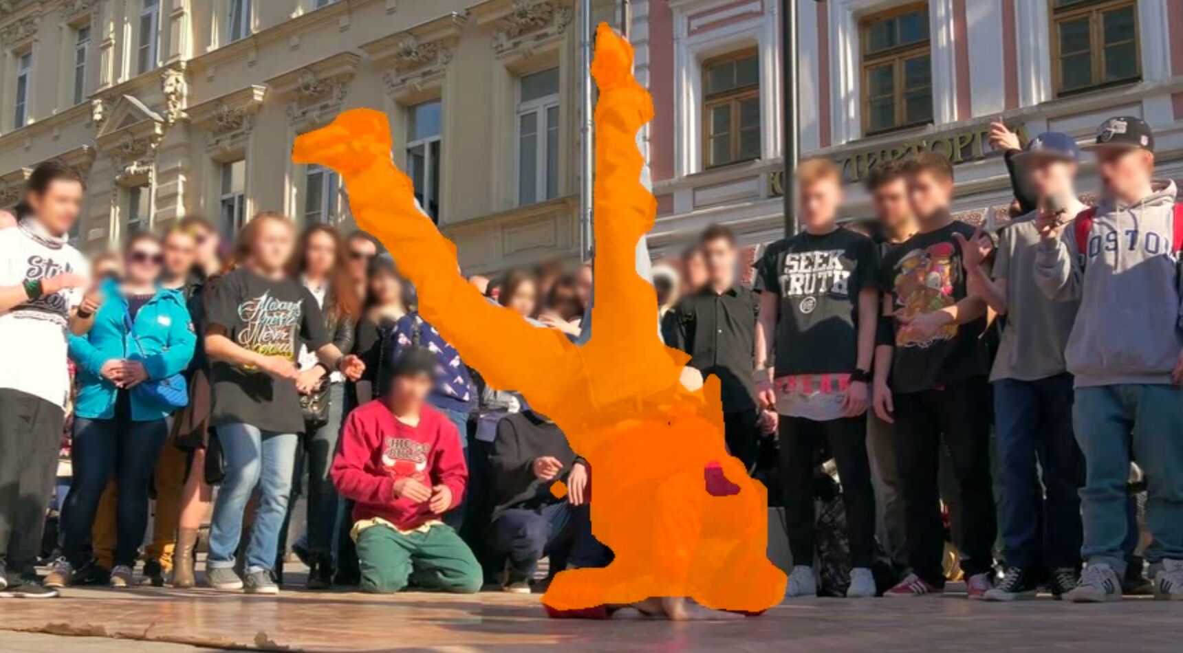
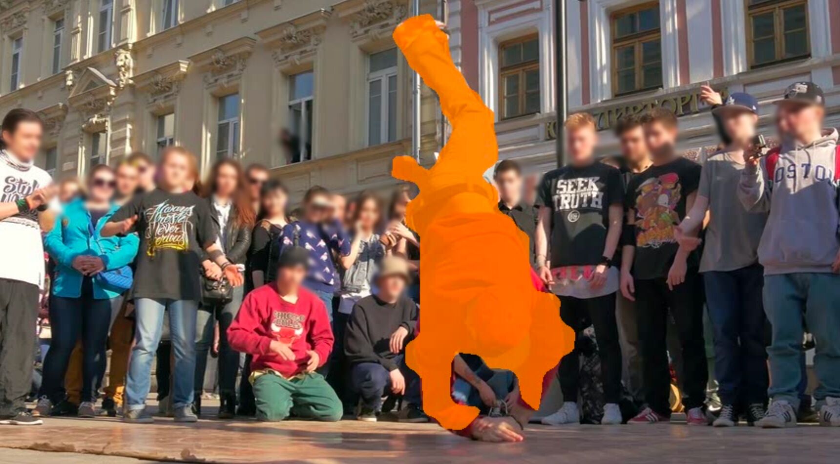
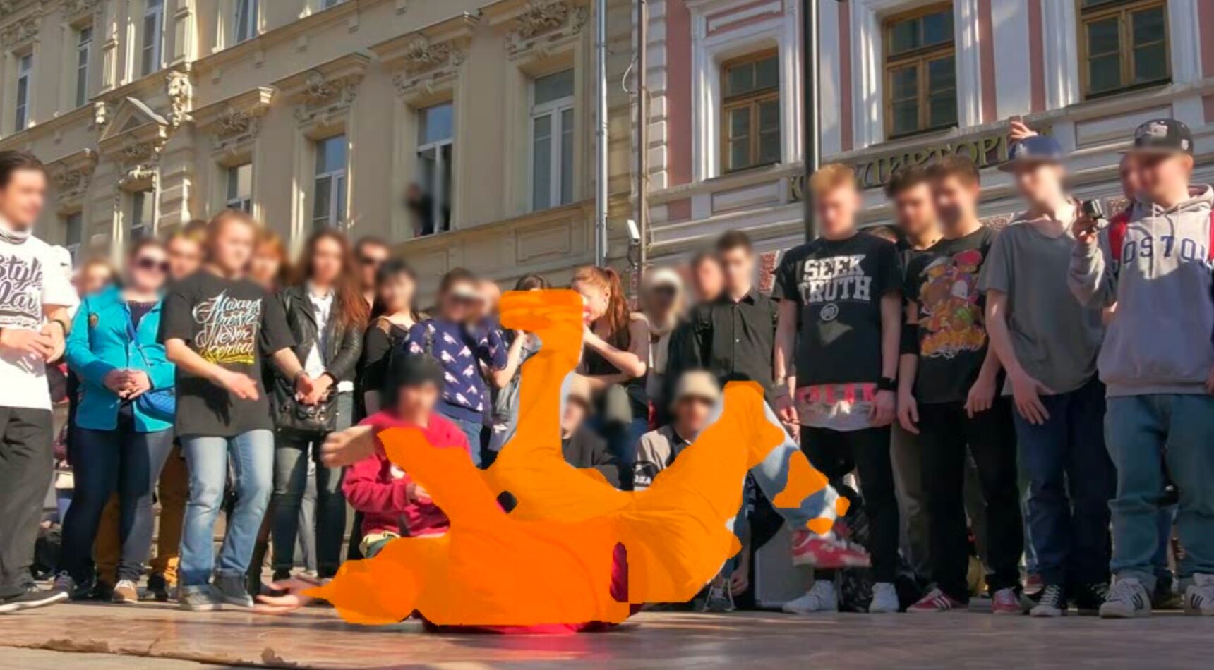
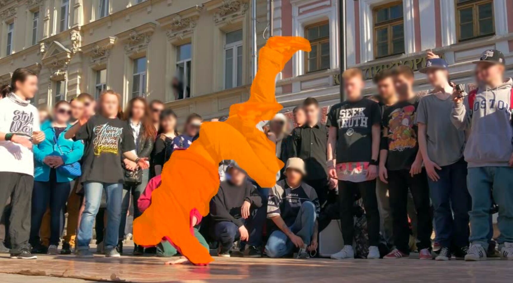
A ground-truth mask is supplied in the first frame, then propagated through later frames. The evaluation tests correspondence conditioned on that initial annotation, rather than discovering objects without labels.
Evaluation protocol.
A nonparametric matcher propagates labels using local cosine similarities between frozen patch features. Context length, neighborhood and temperature are tuned on training data. No learned segmentation head is added, but the matching procedure has selected hyperparameters.
Results.
The reported results improve on prior video encoders and approach, but do not exceed, the selected DINOv 3 comparison. They support useful temporal correspondence under the stated mask-propagation protocol.
3.7 Video and Image Classification
Global image and action recognition checks that the improved dense features have not displaced semantic information. Comparisons include systems with different data and probe designs.
| Method | Param. | Motion Understanding | Appearance Understanding | ||
| SSv2 | Diving-48 | K400 | IN1K | ||
| Results Reported in the Literature | |||||
| VideoMAEv2 (Wang et al., 2023) | 1B | 56.1 | – | 82.8 | 71.4 |
| InternVideo2-1B (Wang et al., 2024b) | 1B | 67.3 | – | 87.9 | – |
| VideoPrism (Zhao et al., 2024) | 1B | 68.5 | 71.3 | 87.6 | – |
| DINOv3 ViT-H+ (Siméoni et al., 2025) | 0.8B | 69.8 | – | 86.7 | 87.9 |
| DINOv3 (Siméoni et al., 2025) | 7B | 70.1 | – | 87.8 | 88.4 |
| Image Encoders Evaluated Using the Same Protocol | |||||
| DINOv2 (Darcet et al., 2023) | 1.1B | 50.7 | 82.5 | 83.6 | 86.1 |
| PEcore G (Bolya et al., 2025) | 1.9B | 55.4 | 76.9 | 88.5 | 87.6∗ |
| SigLIP2 (Tschannen et al., 2025) | 1.2B | 49.9 | 75.3 | 87.3 | 88.0 |
| Video Encoders Evaluated Using the Same Protocol | |||||
| InternVideo22s-1B (Wang et al., 2024b) | 1B | 69.7 | 86.4 | 89.4 | 85.8 |
| V-JEPA ViT-H (Bardes et al., 2024) | 600M | 74.3 | 87.9 | 84.5 | 80.0 |
| V-JEPA 2 ViT-g (Assran et al., 2025) | 1B | 77.3 | 90.2 | 87.3 | 85.1 |
| V-JEPA 2.1 ViT-g | 1B | 76.9 | 89.0 | 87.0 | 84.8 |
| V-JEPA 2.1 ViT-G | 2B | 77.7 | 89.2 | 87.7 | 85.5 |
Task.
Motion-sensitive and appearance-oriented datasets probe different capabilities. Some additional published baselines use related frozen protocols but different attention heads, so the comparisons are not uniformly controlled.
Evaluation protocol.
Four trained attention blocks read frozen encoder features. Predictions are averaged across sampled video clips. This measures encoder features together with a supervised readout and temporal coverage.
Results.
The largest model reaches 77.7% top-one accuracy on Something-Something-v 2 while remaining competitive on appearance tests. The empirical result shows that dense and global performance can coexist in this recipe.
3.8 Video Question Answering
Video question answering adds a language model and paired-data alignment to the frozen visual representation.
| Method | Params Enc / LLM | Avg. |
PerceptionTest Test Acc |
Paired-Acc |
TempCompass multi-choice |
Acc |
TVBench Acc |
MVBench Acc | |
| Video Language Models Results Reported in the Literature | |||||||||
| InternVL-2.5 (Chen et al., 2024) | 300M/7B | 52.1 | 68.9 | 39.9 | 68.3 | 24.3 | 29.4 | 61.6 | 72.6 |
| Qwen2VL (Wang et al., 2024a) | 675M/7B | 47.0 | 66.9 | 29.2 | 67.9 | 20.4 | 31.5 | 46.0 | 67.0 |
| Qwen2.5VL (Qwen Team et al., 2025) | 1B/7B | 49.7 | 70.5 | 36.7 | 71.7 | 24.5 | 24.6 | 50.5 | 69.6 |
| PLM 8B (Cho et al., 2025) | 1B/8B | 56.7 | 82.7* | 39.7 | 72.7 | 28.3 | 33.2 | 63.5 | 77.1 |
| VJEPA 2 ViT-g384 (Assran et al., 2025) | 1B/8B | 59.5 | 84.0* | 44.5 | 76.9 | 36.7 | 40.3 | 60.6 | 73.5 |
| Models trained in this paper using filtered Perception LM data (Cho et al., 2025) | |||||||||
| VJEPA 2 ViT-g384 | 1B/8B | 57.8 | 80.1 | 40.9 | 74.1 | 32.3 | 41.4 | 62.6 | 73.3 |
| VJEPA 2.1 ViT-G384 | 2B/8B | 57.9 | 83.1 | 43.2 | 74 | 28.5 | 38 | 62.8 | 75.4 |
Task.
The comparison restricts language backbones to roughly eight billion parameters and includes physical, temporal and general video-question benchmarks. Their task biases differ.
Evaluation protocol.
Paired training data is filtered using several criteria, including an external multimodal model as a quality judge. Progressive alignment adds longer-context training and a final PerceptionTest stage. Language-free visual pretraining therefore does not imply a question-answering system free of language supervision.
Results.
Under the new alignment data, V-JEPA 2.1 improves several benchmarks but declines on TemporalBench and TOMATO relative to the rerun V-JEPA 2. Its overall scores are competitive rather than uniformly better; older headline results also used a larger alignment corpus.
| Image | DINOv2 | DINOv3 | V-JEPA 2 | V-JEPA 2.1 |
|
|

|

|
|
|
|

|

|
|
|
|

|

|

|

|
|

|

|

|

|
|

|

|

|

|
|

|

|

|

|
|
|
|

|

|

|

|

|

|

|
|
|

|

|
|
|

|

|

|

|



















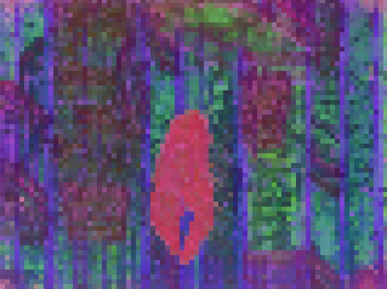
3.9 Qualitative results of V-JEPA 2.1 Dense Features
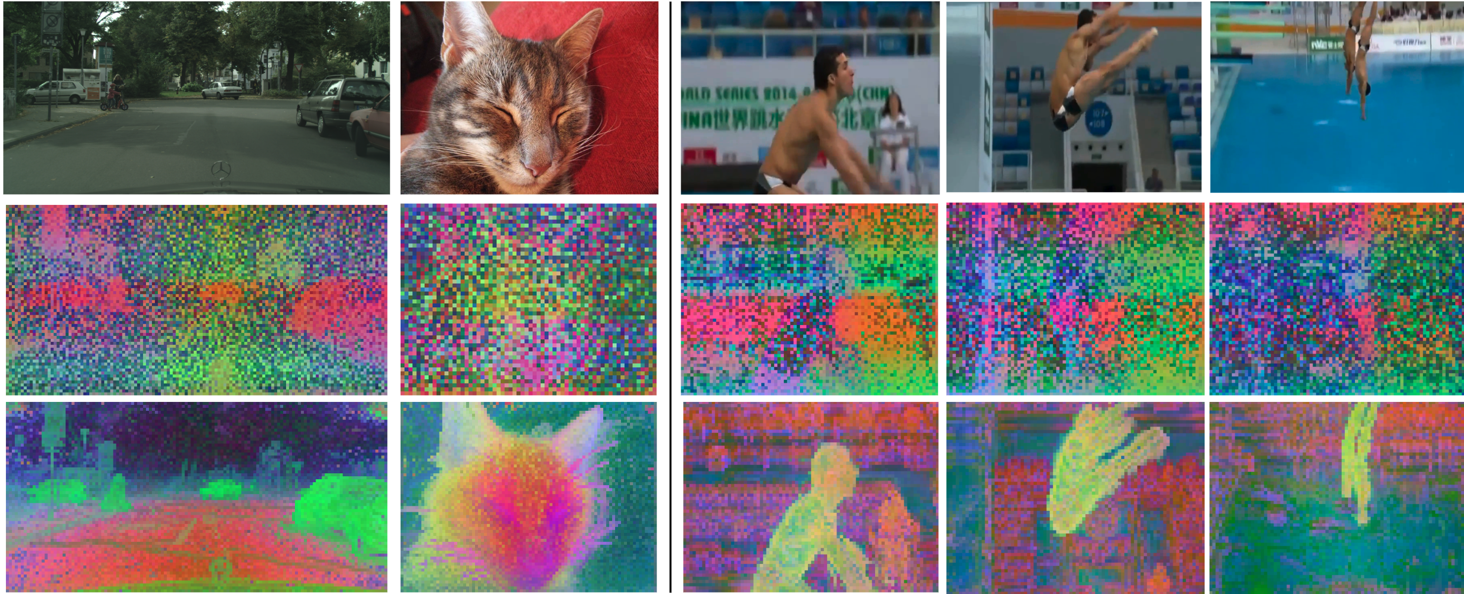
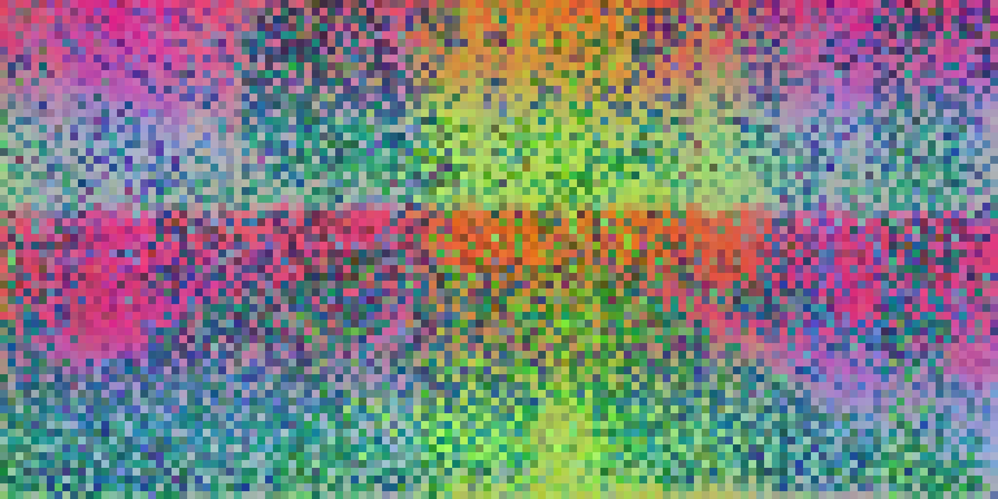
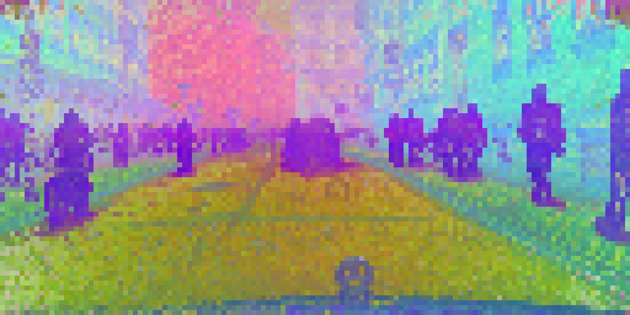
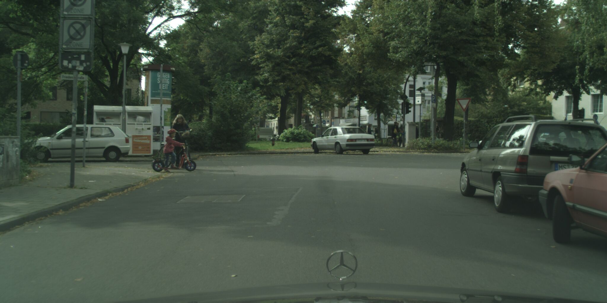
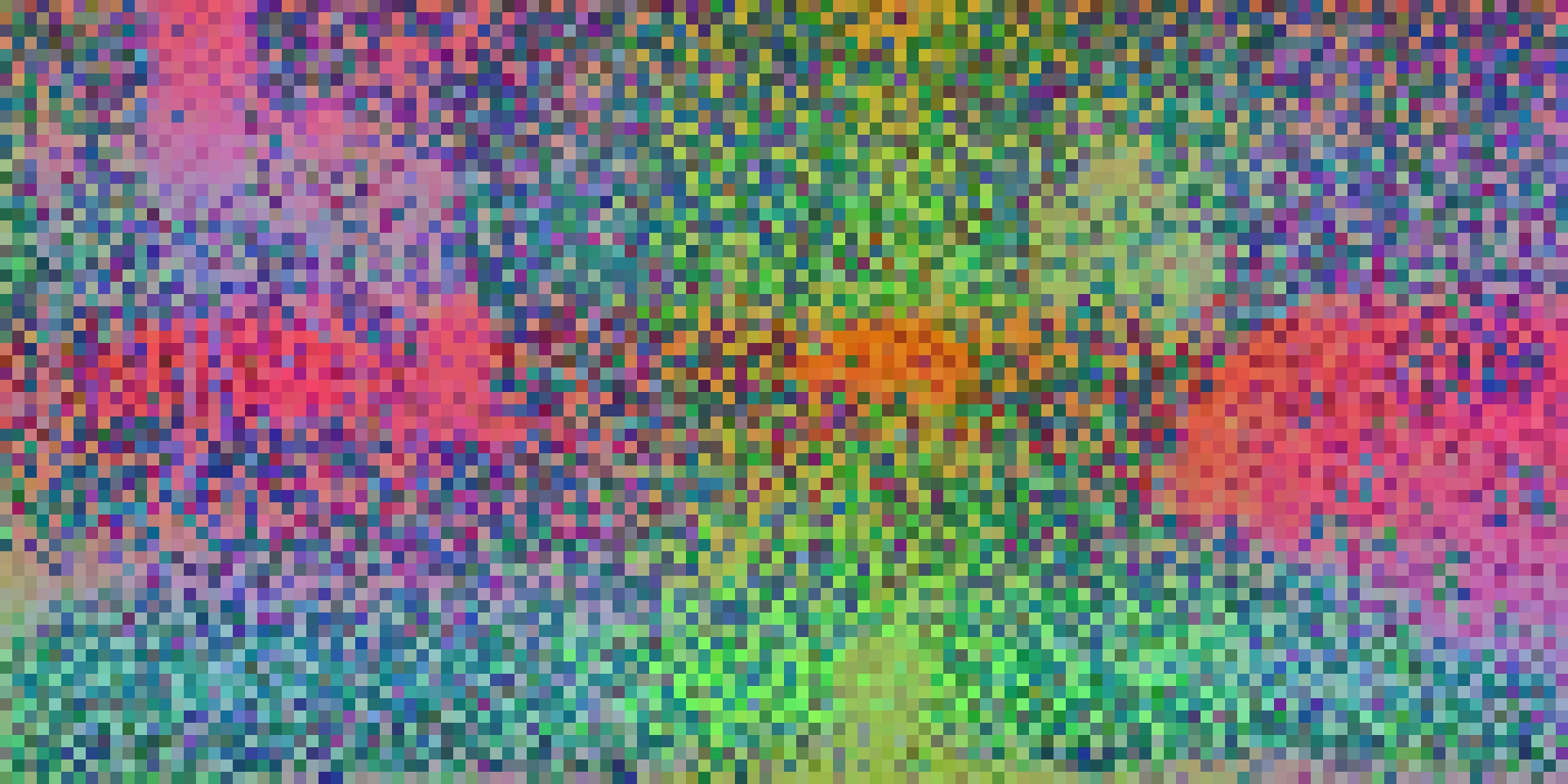
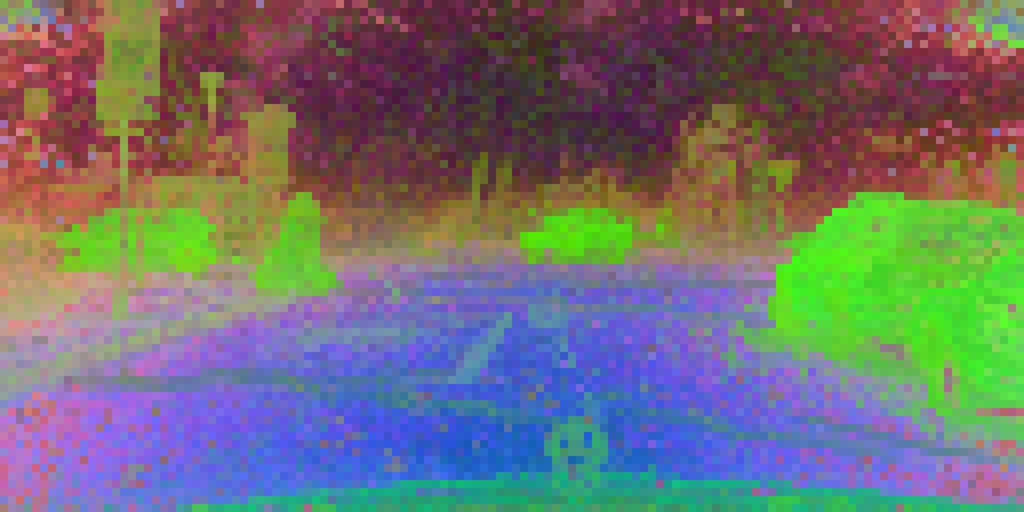
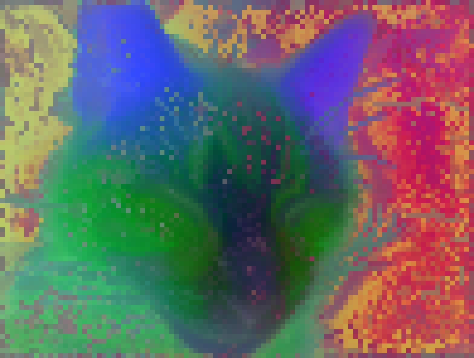
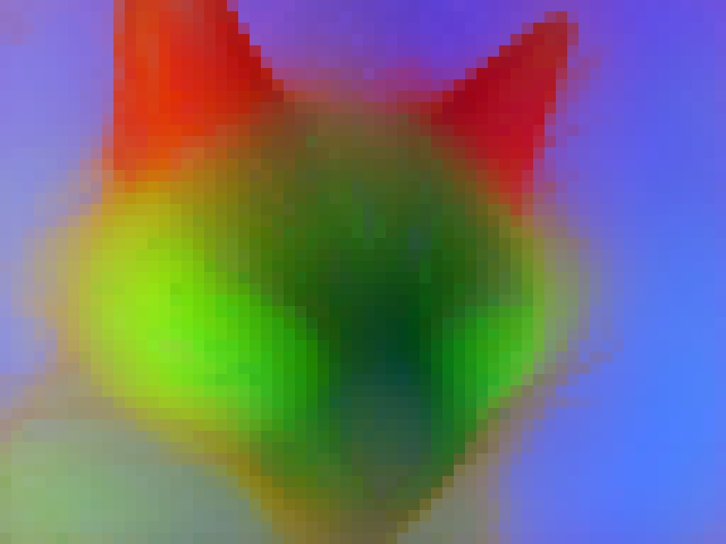
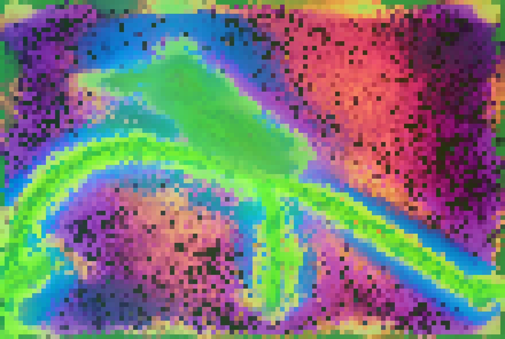
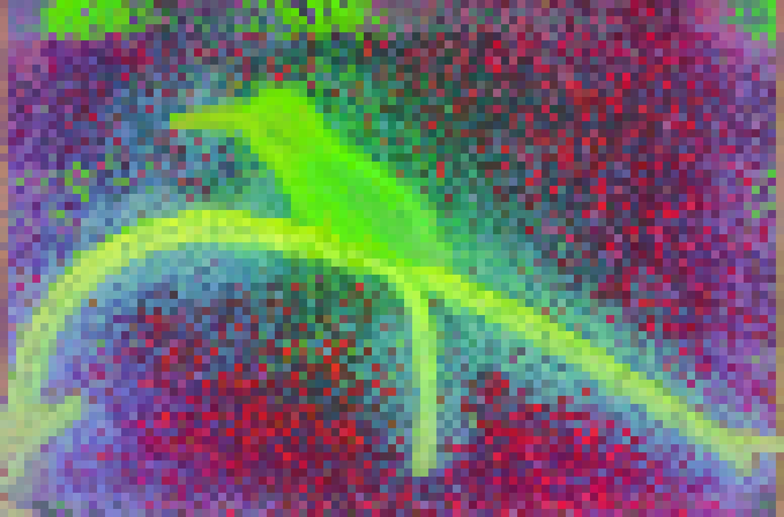
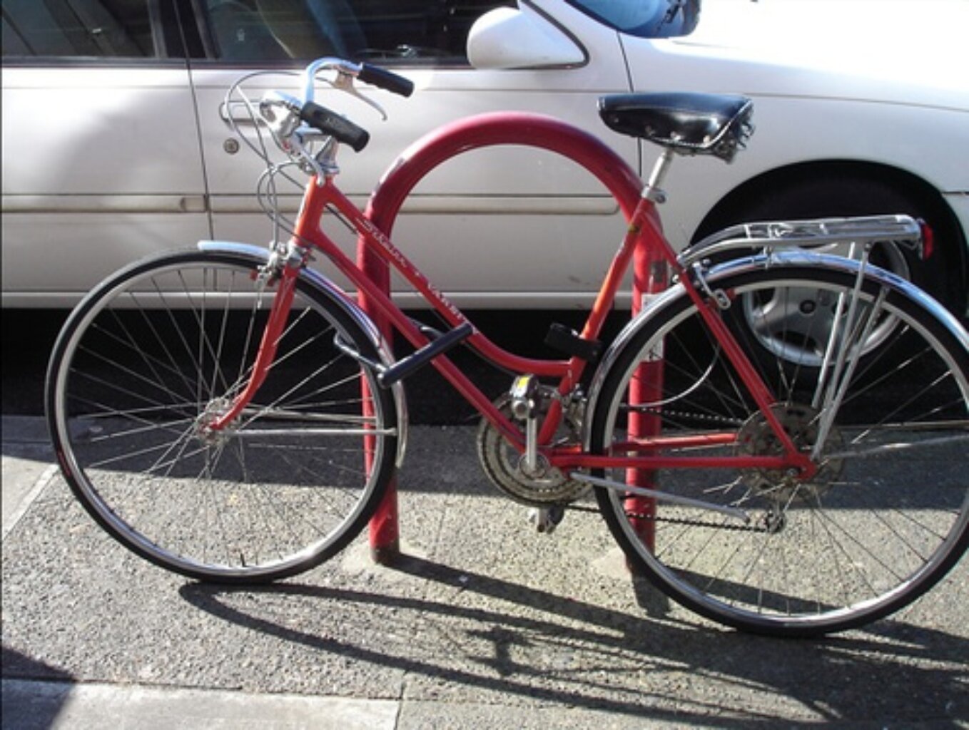
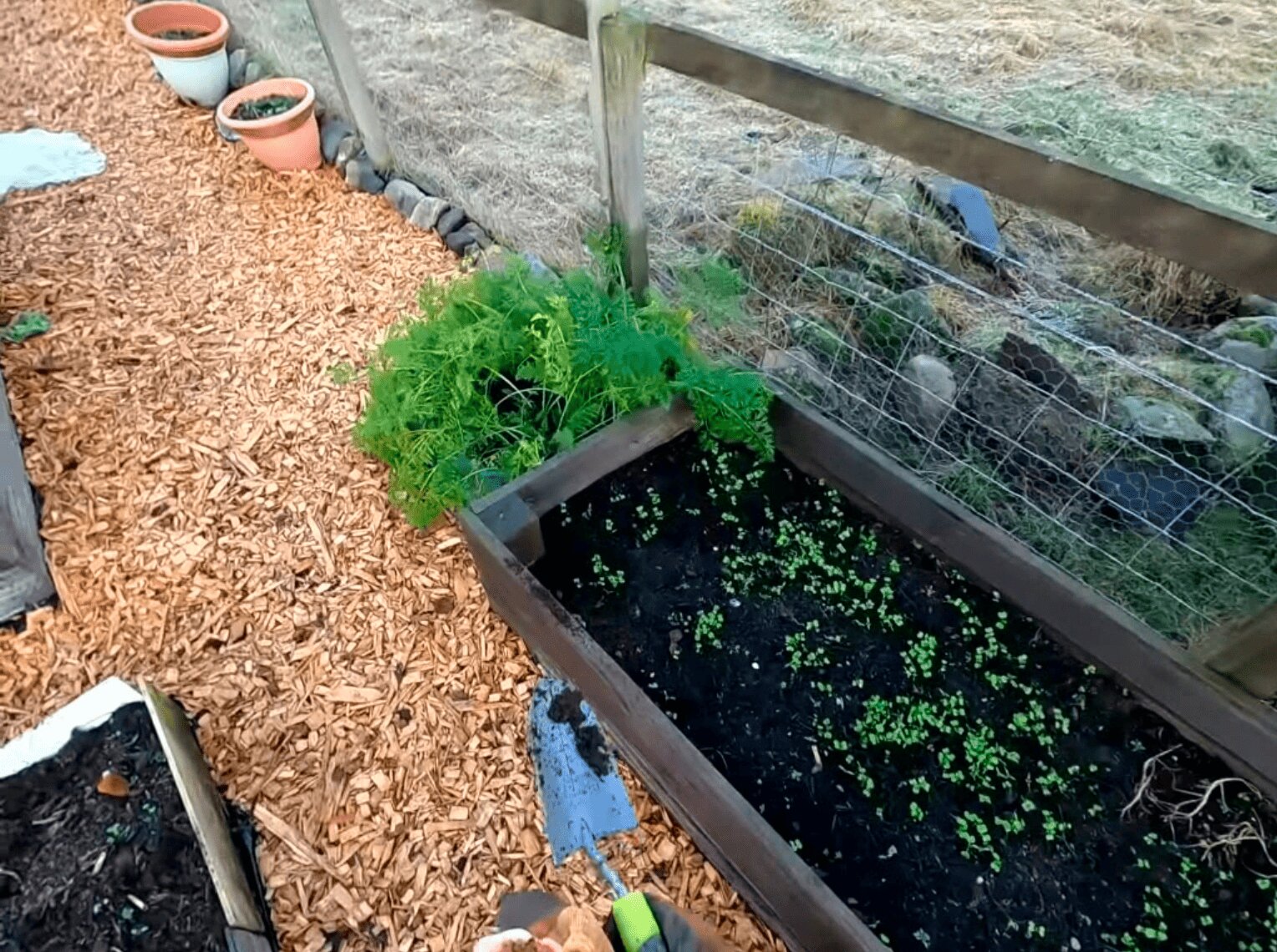
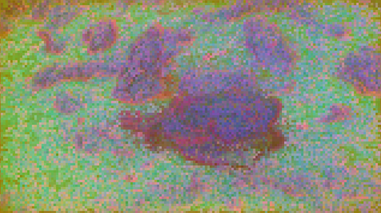
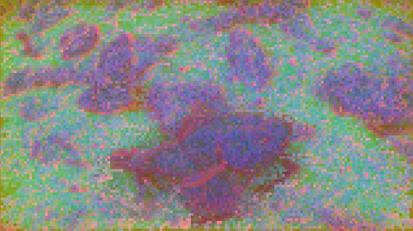
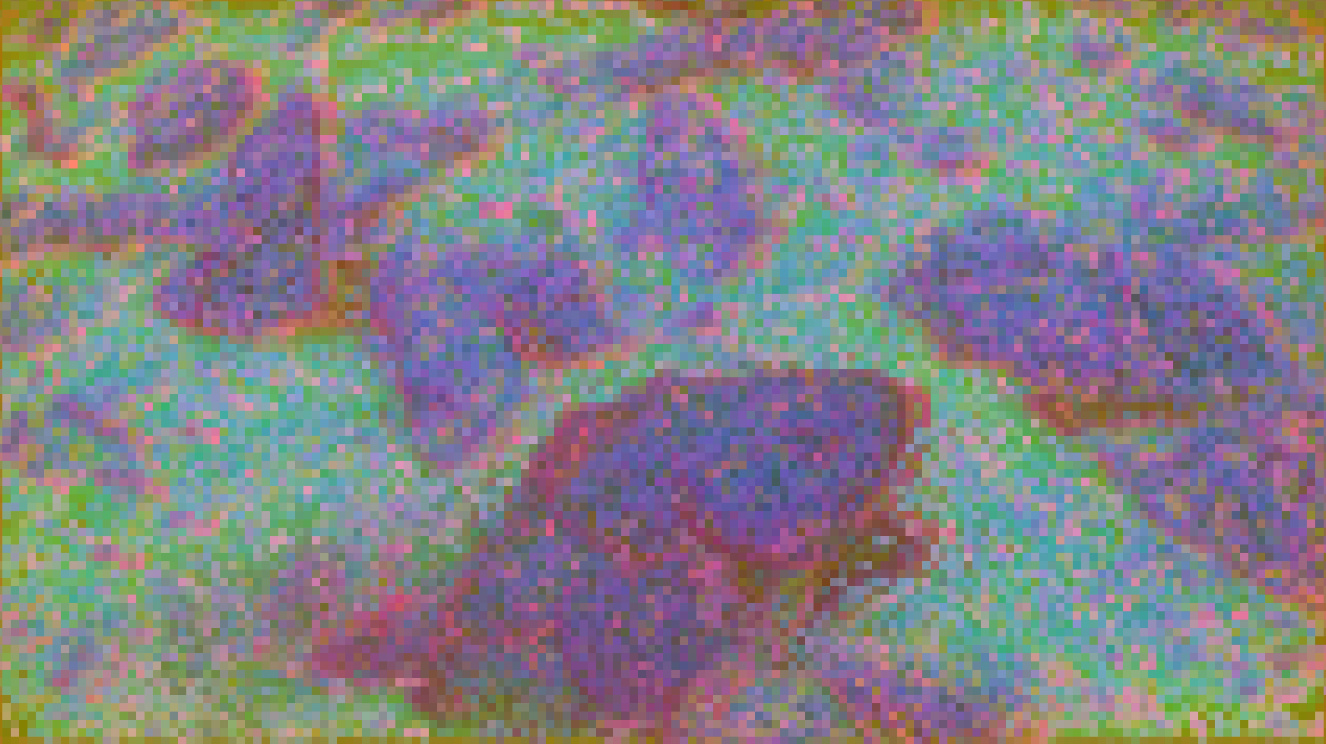
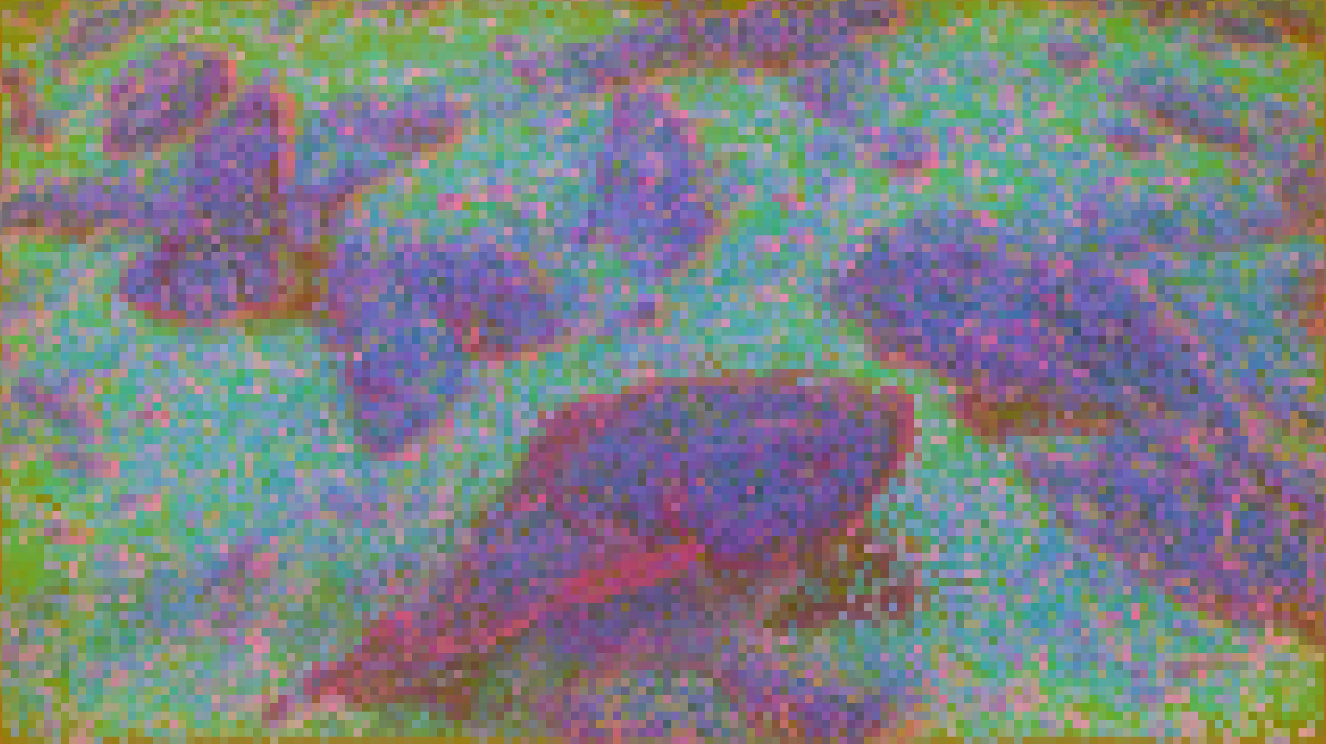
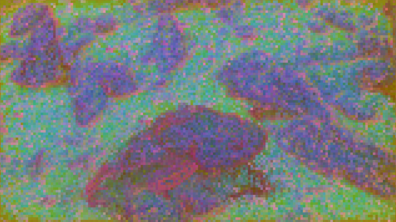
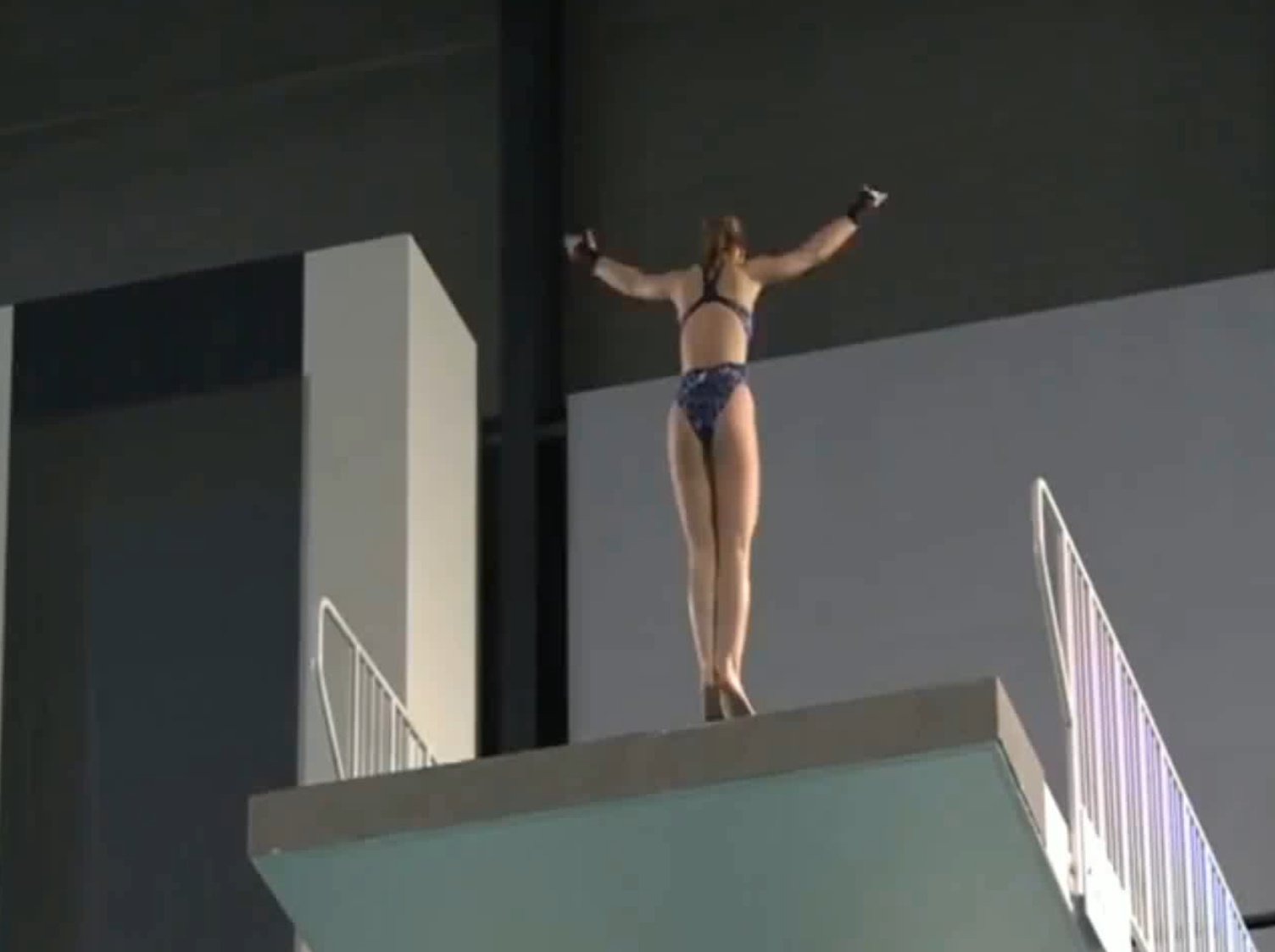
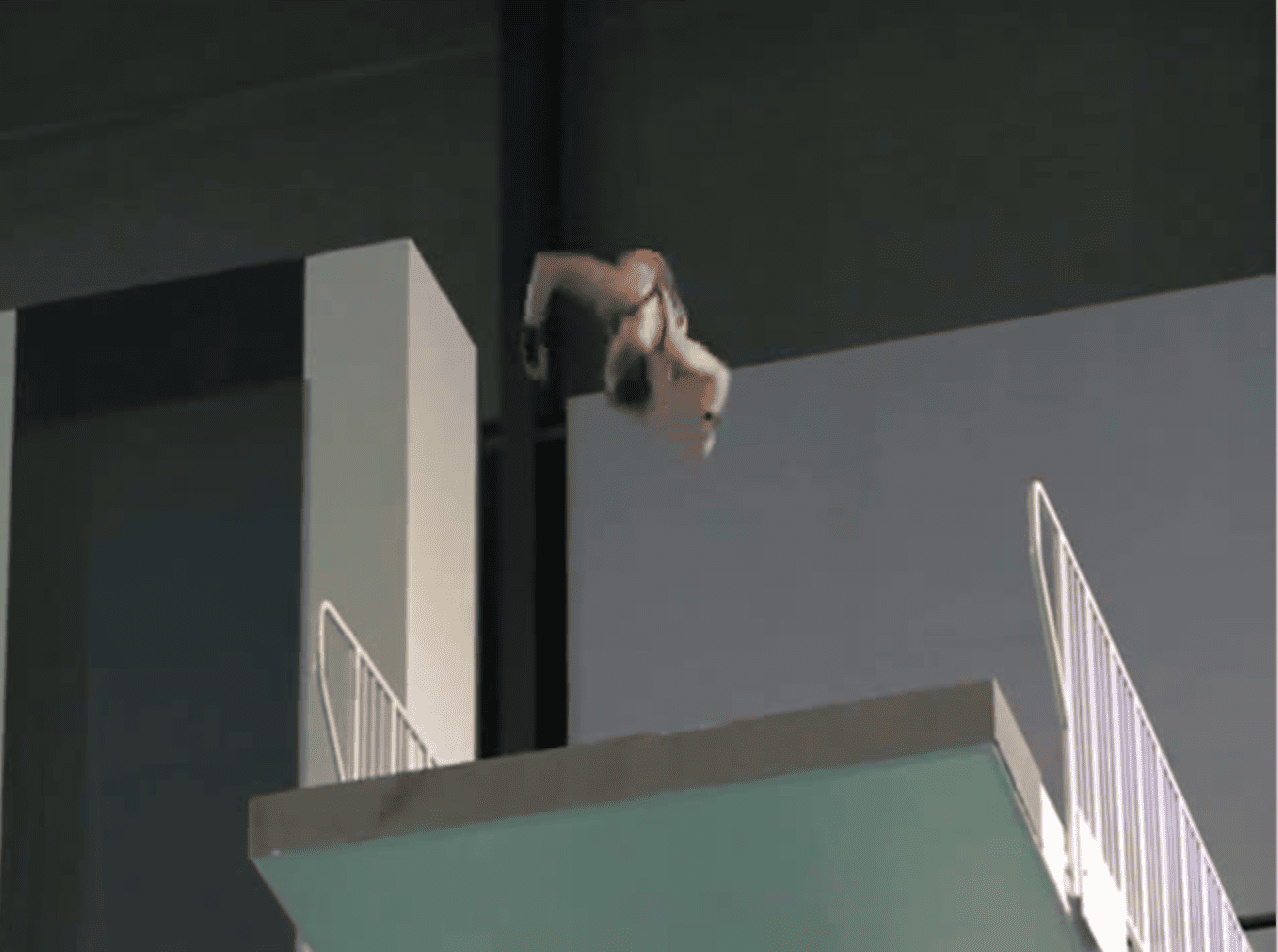
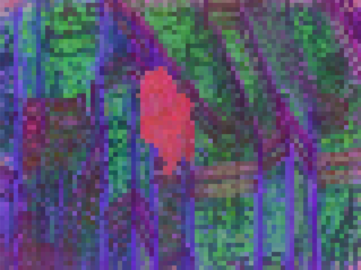
PCA maps visualize local spatial and temporal coherence. The authors select visually appealing RGB component permutations, so these are qualitative illustrations rather than calibrated segmentation outputs. The full image and video comparisons are retained below.
3.10 Family of distilled models
Distilled models improve substantially over same-size models trained from scratch. The larger teacher’s training cost and data are part of that route to compact models; parameter count at deployment does not represent the entire training budget.
| Model | Params | Distilled | SSv2 | K400 | IN1K | ADE20K | Citys. | VOC12 | NYU () | KITTI () | DAVIS |
| ViT-G | 2B | 77.7 | 87.7 | 85.5 | 47.9 | 73.5 | 85.0 | 0.307 | 2.461 | 69.0 | |
| ViT-L | 300M | 74.2 | 84.3 | 81.8 | 42.0 | 66.7 | 79.6 | 0.381 | 2.914 | 64.5 | |
| ViT-L | 300M | ✓ | 76.5 | 86.9 | 84.9 | 46.7 | 71.0 | 83.9 | 0.336 | 2.490 | 68.7 |
| ViT-B | 80M | ✓ | 74.5 | 85.1 | 84.0 | 42.0 | 64.5 | 78.0 | 0.408 | 2.850 | 67.0 |
4 Related work
Self-Supervised Learning.
The work builds on transformation-invariant, contrastive, non-contrastive and masked-modeling approaches. Its focus is where and how to apply latent prediction supervision to make features useful locally as well as globally.
Video Models.
Video-learning history includes supervised recognition, temporal pretext tasks, reconstruction and latent prediction. Scaling observation data makes broadly useful encoders possible, but does not by itself specify the best local representation or control objective.
Learning dense features.
Dense representation learning uses local consistency, region-based losses, distillation and spatial decoders. V-JEPA 2.1 emphasizes direct context supervision and intermediate targets; its comparisons should be read alongside these established alternatives.
5 Conclusion and Future work
The full recipe improves accessible local structure while preserving strong recognition. Its evidence combines matched component studies with larger system comparisons. Downstream supervision, curated data and separate planning heads remain part of the demonstrated capabilities.
Future work.
Larger models, more data and richer world-model applications remain future directions. Better dense features are a useful building block, not a complete solution to autonomous-agent perception, planning or control.
Appendix A Pretraining details
The primary training phase uses short, low-resolution clips and native images; cooldown increases duration and resolution. Image/video batch sizes, fixed target averaging, context-loss weights and the 24-block predictor are specified. These details distinguish the complete recipe from merely adding an unweighted visible-token loss.
| Parameter | Primary Phase | Cooldown Phase |
| Number of frames | 16 | 64 |
| Frames per Second | 4.0 | 4.0 |
| Video Crop Size | 256 | 384 |
| Image Crop Size | 256 | 512 |
| Random Resize Aspect Ratio | [0.75, 1.35] | [0.75, 1.35] |
| Random Resize Scale | [0.3, 1.0] | [0.3, 1.0] |
| Steps | 135,000 | 12000 |
| Warmup Steps | 12,000 | N/A |
| Image batch Size (global) | 2,304 | 2,304 |
| Video batch Size (global) | 128 | 128 |
| Starting Learning Rate | 1e-4 | 6e-4 |
| Final Learning Rate | 5.25e-4 | 1e-6 |
| Weight Decay | 0.04 | 0.04 |
| EMA | 0.99925 | 0.99925 |
| Spatial Mask Scale | [0.15, 0.7] | [0.15, 0.7] |
| Temporal Mask Scale | [1.0, 1.0] | [1.0, 1.0] |
| Mask Aspect Ratio | [0.75, 1.5] | [0.75, 1.5] |
| Tubelet Size | 2 | 2 |
| Patch Size | 16 | 16 |
| Predictor Blocks | 24 | 24 |
| Predictor Embedding Size | 384 | 384 |
| Encoder Intermediate Blocks (ViT-G) | [12, 24, 36, 48] | [12, 24, 36, 48] |
| Context Loss | 0.5 for video, 0.7 for image | 0.5 for videos, 0.7 for images |
Appendix B Distillation details
Distillation replaces the moving target encoder with a frozen teacher and trains a fresh 12-block predictor using final-layer targets. A separate averaged student becomes the released model. The teacher and student both pass through low- and high-resolution phases, with the second student stage initialized from the first averaged student.
Appendix C Evaluation protocols
C.1 Depth Estimation
Datasets and Metrics.
Depth is evaluated on NYUv 2 and KITTI using root-mean-square error. The metric’s scale depends on the dataset and depth protocol.
Evaluation Protocol.
A trained linear readout and learned normalization sit above frozen image features. Hyperparameters are swept. This remains supervised depth probing, even though the encoder was pretrained without depth labels.
C.2 Semantic Segmentation
Datasets and Metrics.
Semantic segmentation uses class labels on VOC12, ADE20K and Cityscapes and reports average overlap per class.
Evaluation Protocol.
A linear head reads final-layer frozen patch features with dataset-specific image resolution. Learning rate and weight decay are selected from explicit sweeps.
C.3 Video Object Segmentation Tracking
Dataset and Metrics.
DAVIS uses its established train/validation videos. For YouTube-VOS, the authors split publicly available training videos into their own 80/20 training/validation partition; this differs from an official held-out test submission.
Evaluation Protocol.
The first annotation is propagated through cosine-similar patches from the initial and recent frames. Hyperparameters are selected on DAVIS training data before application to validation sets. This nonparametric evaluation still depends on that selected matching procedure.
C.4 Short Term Object Interaction Anticipation
Dataset and Metrics.
The strict combined anticipation metric requires spatial overlap, noun, verb and contact timing within a tolerance. Its top-five rule discounts some plausible alternative predictions, which is important for understanding the reported mAP.
Evaluation Protocol.
Frame-guided pooling aligns video features with high-resolution last-frame features before a supervised detection head. This supplies both temporal context and fine spatial detail.
Probe Architecture.
Region proposals and aligned local features feed noun, verb and time-to-contact outputs. Global pooled context supplements local features. The trained head adds detection, verb and timing losses above the frozen encoder.
Optimization.
The appendix sweeps temporal span, sampling rate, spatial resolution and optimization settings before reporting selected configurations. Its final clip setting differs from the illustrative main-text description; reproduce the complete chosen protocol rather than assuming one fixed input setup throughout.
C.5 Video and Image Classification
Dataset and Metrics.
ImageNet and several action datasets supply supervised labels for frozen classification probes. Reported classification accuracy belongs to these dataset-specific tasks.
Probe Architecture.
The readout consists of attention blocks, a learned query and a final classifier above frozen encoder features.
Evaluation Protocol.
Clip counts and spatial views differ by task. Diving-48 also uses features from several encoder layers. Temporal coverage and feature extraction choices are part of the evaluation recipe.
Optimization.
Several heads with different learning rates and regularization are trained, and the best is reported. Some tasks train longer than others.
C.6 Action Anticipation
Dataset and Metrics.
EPIC-KITCHENS anticipation uses a fixed kitchen-action vocabulary and mean-class recall at five. Its default validation gap is one second.
Evaluation Protocol.
The supervised head uses focal loss and samples anticipation timing during training. The visual encoder and predictor supply features under the stated fixed-resolution context protocol.
Appendix D Additional Ablations
D.1 Multi-scale evaluation
Deep supervision narrows the gap between using only final-layer features and combining several encoder layers. The effect varies by task and does not mean intermediate features are never useful.
D.2 Pretraining Spatial Resolution
Higher cooldown spatial resolution improves the tested downstream tasks. These results isolate a practical training-resolution choice within the full recipe.
| Model | Res | SSv2 | D-48 | K400 | IN1K | EK100 | ADE20k | Citys. | VOC | NYU | KITTI | DAVIS | YT-VOS |
| ViT-g | 256 | 76.7 | 88.6 | 86.2 | 84.1 | 35.7 | 47.8 | 71.7 | 84.6 | 0.359 | 2.611 | 68.0 | 72.0 |
| ViT-g | 384 | 76.9 | 89 | 87 | 84.8 | 38.4 | 47.8 | 71.8 | 84.7 | 0.350 | 2.601 | 67.4 | 71.3 |
| ViT-G | 256 | 77.1 | 89.5 | 87.3 | 84.8 | 38.8 | 47.8 | 73.2 | 84.7 | 0.313 | 2.472 | 68.6 | 72.7 |
| ViT-G | 384 | 77.7 | 89.2 | 87.7 | 85.5 | 40.8 | 47.9 | 73.5 | 85.0 | 0.307 | 2.461 | 69.0 | 72.6 |