At a glance
Intuition: a route around a wall can look short in a visual feature space even though it is physically far away. This paper trains a JEPA encoder and predictor while encouraging consecutive latent movements to point in similar directions. The resulting geometry gives gradient-based planners a more useful goal-distance signal in simulated navigation and pushing. A linear-systems analysis connects near-identity transitions to the conditioning of action optimization. That theory is conditional: the cosine penalty only controls visited directions under additional assumptions, and it does not prove global convexity for nonlinear models. Experiments show stronger planning with fewer search computations, while long horizons and asymmetric dynamics remain difficult.
1 Introduction
A good image representation need not be a good planning representation. Visual similarity can ignore walls or make progress toward a goal hard to measure. The proposed regularizer reshapes the representation during predictive training, aiming to make local trajectory directions more consistent and action optimization easier.


2 Related Work
The method is part of the JEPA world-model family and directly extends frozen-feature planning. Unlike a temporal contrastive objective, it does not push distant-in-time frames apart or require negative pairs. Unlike pixel reconstruction, it targets trajectory geometry. These differences motivate the design; measured comparisons are needed to establish when it helps.
3 Temporal Straightening
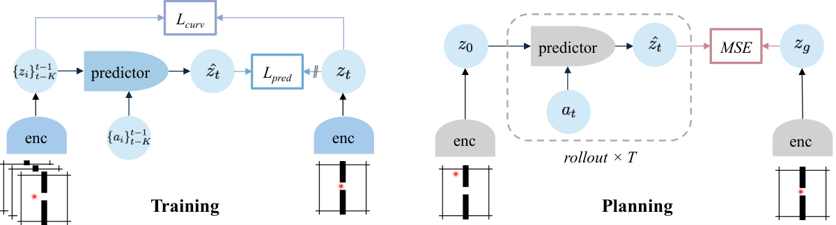
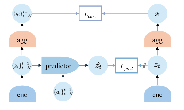
The system learns observation features, action features and a future predictor from offline trajectories. Straightening is an additional geometric objective, separate from prediction and collapse prevention.
3.1 World Model
Three modules connect observations and actions to future latent states. Encoders may retain a spatial feature grid or output one global vector.
Sensory encoder.
The observation encoder chooses the state space in which both prediction and planning occur. A learned projector can adapt frozen visual features, or an image encoder can be trained from scratch.
Equation 1
| (1) |
Action encoder.
An action encoder transforms physical control inputs into features suitable for the predictor. It does not itself choose actions.
Equation
Predictor.
The predictor uses a history of encoded states and actions to forecast the next state. At deployment its own predicted states supply later context, so long-rollout errors can accumulate.
Equation 2
| (2) |
3.2 Straightening Latent Trajectories
Subtract adjacent latent states to obtain approximate movement vectors, then maximize the cosine between consecutive movements. This penalizes changes in direction rather than simply shrinking every step. The desired straightness is local along observed trajectories, not a requirement that all possible routes lie on one line.
Equations 3–4
| (3) |
| (4) |
3.3 Training Objective.
Prediction and curvature losses jointly train the modules. Their relative weight controls how strongly the state geometry is reshaped.
Prediction objective.
Squared error matches predicted next features to target features whose gradients are stopped. The targets are produced by the learned representation rather than annotated physical states.
Equation 5
| (5) |
Straightening objective.
One minus cosine similarity is small when adjacent latent displacements point the same way. It is invariant to uniform scaling of those displacement vectors and therefore does not independently require a large informative representation.
Equation 6
| (6) |
Overall objective.
A nonnegative weight combines curvature and predictive accuracy. Excessive geometric pressure could remove useful changes; the empirical setting of this weight matters.
Equation 7
| (7) |
Collapse prevention.
Stop-gradient is used in most experiments, but a constant representation remains theoretically possible. Straightening is not an anti-collapse guarantee. It can be combined with other regularization or contrastive methods; successful training here is empirical.
4 Planning with Straightened Dynamics
For linear latent dynamics, the terminal goal loss is quadratic in the action sequence. Its nonzero Hessian spectrum matches a controllability Gramian. If the transition is close to identity and actions are well conditioned, the derived bound on optimization conditioning improves. This first assumes square invertible action mapping; low-dimensional actions require controllability conditions on the reachable subspace. High cosine similarity is only a proxy along visited velocities, and nonlinear predictors need further Jacobian and higher-order analysis. The original assumptions and statements are retained.
Equation 8
| (8) |
Assumption 4.1 (Linear latent dynamics).
For analysis, we consider linear latent dynamics
Equation 9
| (9) |
where and . We first state results for and invertible; see Remark 4.5 for .
Definition 4.2 (-straight transition).
Under the linear dynamics, we call -straight if
Equation 10
| (10) |
The term “straight” reflects that, as tends to , the dynamics of approach those of the reference function , where the state evolves linearly along a straight trajectory modified only by the control input. We are primarily interested in the regime where is small.
Remark 4.3 (Cosine similarity as a practical proxy).
In practice, we regularize temporal straightness using the cosine similarity between consecutive latent velocities (4). Under mild bounded-variation assumptions on velocity magnitudes and smooth actions, a large cosine similarity implies that is small along visited velocity directions. Detailed proofs are in Section C.3.
Theorem 4.4 (Conditioning of the planning Hessian).
Under Assumption 4.1 with and invertible, unrolling (9) yields
Equation
so is affine in and the planning Hessian is
Equation
where Let be the finite-horizon controllability Gramian (Kailath, 1980; Sontag, 1998; Chen, 1999). Then the effective condition number satisfies
Equation 11
| (11) | ||||
where . Moreover, if the transition is -straight with , then
Equation 12
| (12) |
For , this gives .
Proofs are in Section C.2.
Remark 4.5 (Low-dimensional actions).
When , is not invertible and (hence ) may be singular outside the controllable subspace. Theorem 4.4 holds on when is computed using ; see Section C.2.
5 Experiments
Four simulated environments cover a wall, two maze complexities and contact-rich pushing. The main comparison adapts DINO-WM-style encoders and uses the same recorded datasets. No real-robot deployment is demonstrated.
5.1 Architecture details
The experiments instantiate the idea with frozen DINOv2 plus a learned projector, or with a learned ResNet, and an action-conditioned transformer predictor.
Visual encoder.
The projector can compress channels or spatial resolution while adapting the features for dynamics. A from-scratch encoder offers more freedom but must learn useful perception from the task data. These are distinct representation setups, not equivalent amounts of pretraining.
Equation 13
| (13) |
Predictor.
Actions and available proprioception are concatenated to visual features. A causal attention mask prevents later observations leaking into earlier predictions. The availability of proprioception changes what physical information the model receives.
Cosine similarity computation.
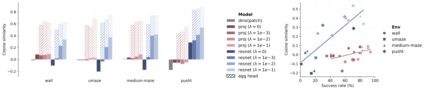
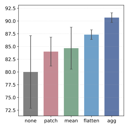
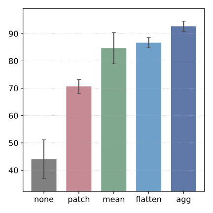
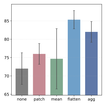
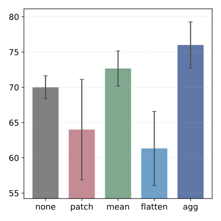
For spatial grids, straightness can be measured patch by patch, after flattening, after pooling or through a learned aggregation head. The main experiments use the last option. The prediction model retains spatial detail while the regularizer shapes a global trajectory signal.



5.2 How good is the embedding space?
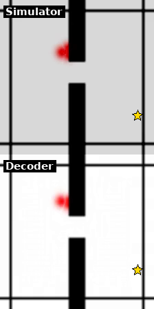
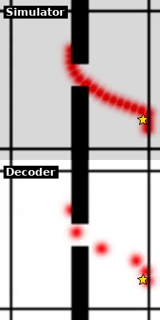
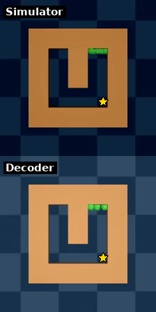
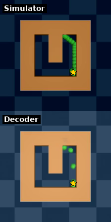
The diagnostics examine curvature, distance-to-goal maps and decoded images. They help explain planning performance but do not themselves prove a representation is sufficient for every task.
Reduced curvature.
Predictive training alone often reduces curvature, and the explicit penalty strengthens that trend. Aggregation allows complex local patch motion without requiring each patch to follow an overly straight path. The explanation connecting this geometry to better search is supported by controlled comparisons, with task-dependent effects.
Faithful distance.
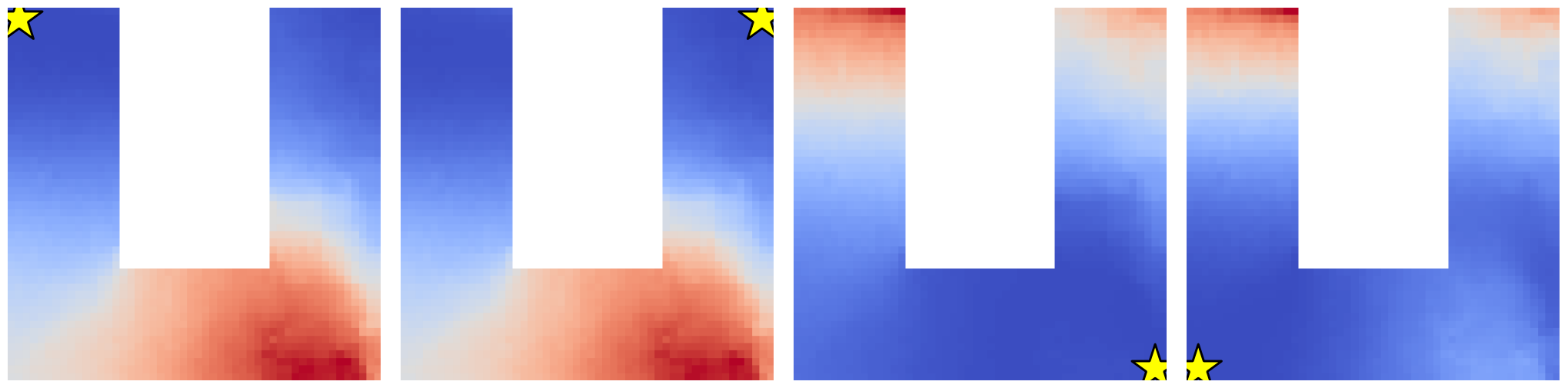
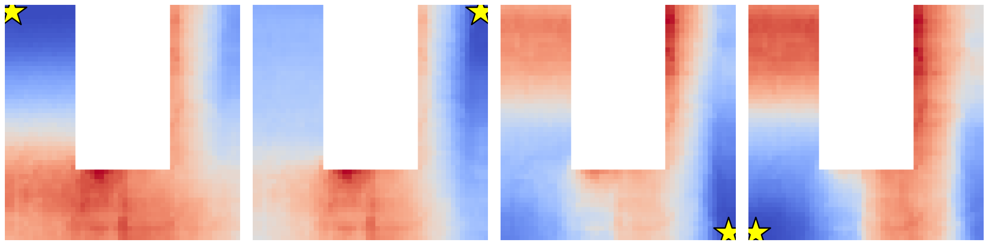
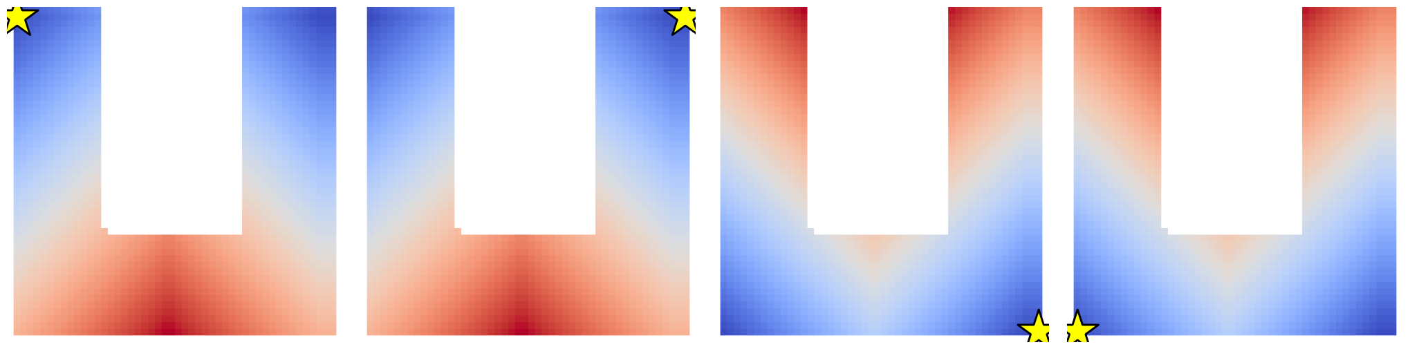
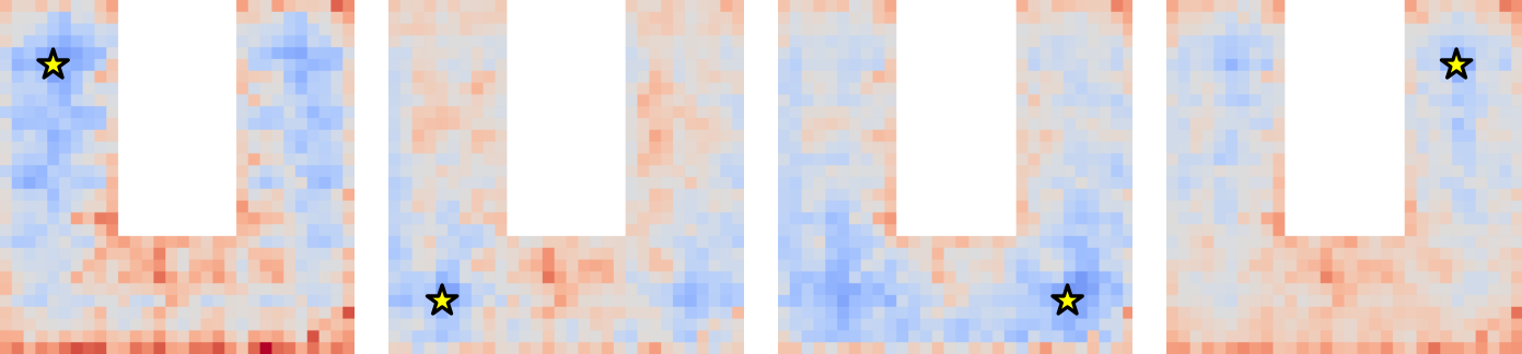
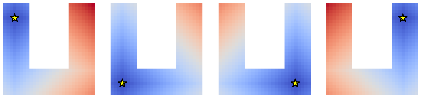
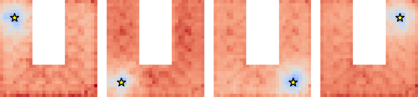
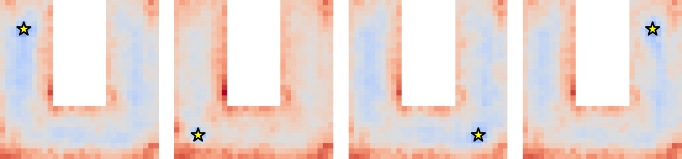
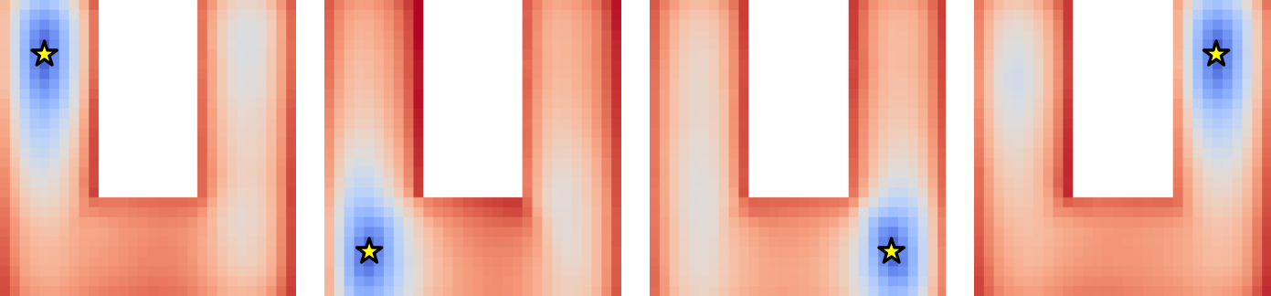
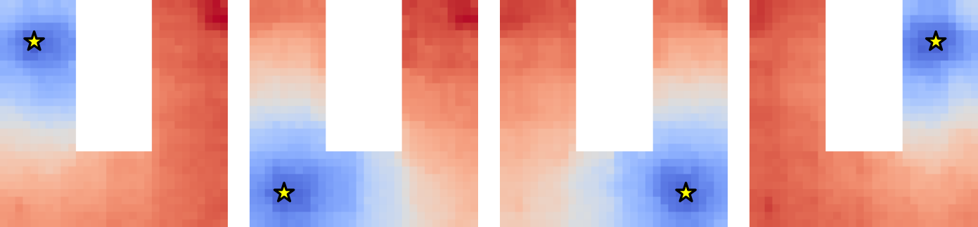
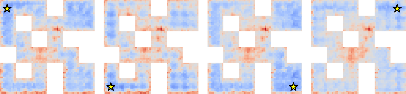
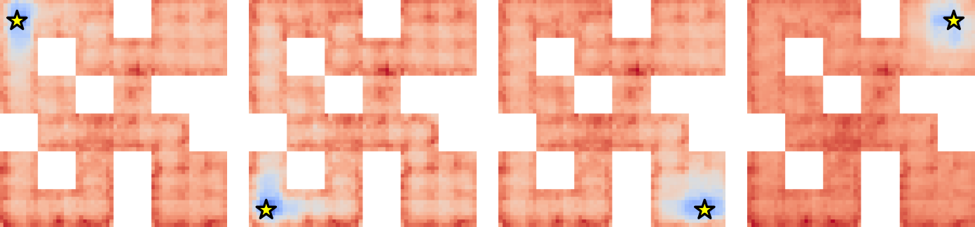
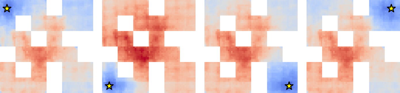
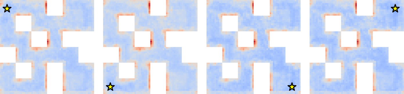
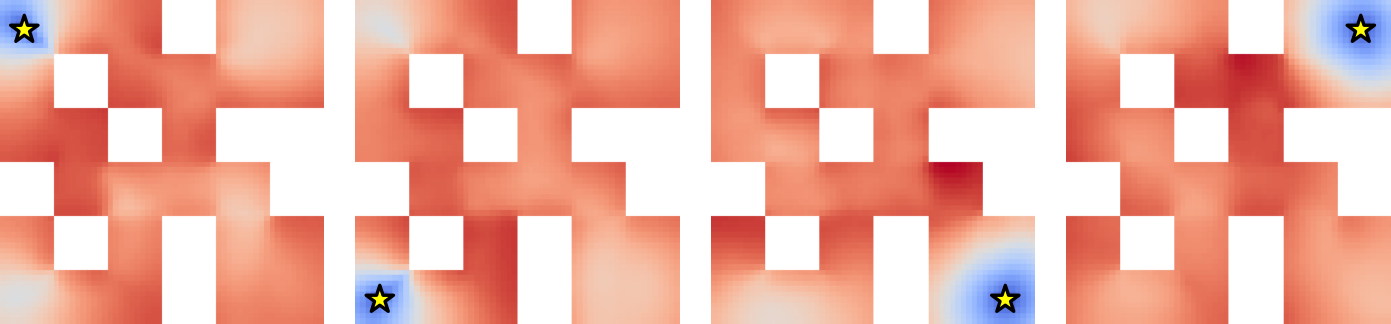
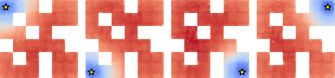
Distance heatmaps are compared with shortest paths on discretized mazes. Straightened features better reflect obstacle-aware progress in those examples. This is empirical alignment with the tested transition graph, not a global theorem identifying geodesic distance from arbitrary videos.
Sufficient information.
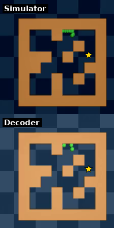
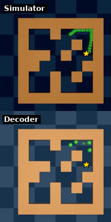
A separately trained detached decoder reconstructs observations from compressed latents. Accurate reconstruction shows retained visual information in these simple scenes, but is neither necessary nor sufficient for successful control. Table 1 reports actual planning outcomes, with regularization strengths selected using held-out validation seeds.
| Encoder | Config | Wall | PointMaze – UMaze | PointMaze – Medium | PushT | |||||
|---|---|---|---|---|---|---|---|---|---|---|
| dim | Open-loop | MPC | Open-loop | MPC | Open-loop | MPC | Open-loop | MPC | ||
| DINOv2 (CLS) | ✗ | 28.67 12.68 | 66.67 10.50 | 25.33 0.94 | 82.67 9.98 | 20.00 8.16 | 67.50 3.54 | 19.33 8.22 | 28.00 1.63 | |
| DINOv2 (patch) + proj | ✗ | 28.67 0.94 | 76.00 4.90 | 34.67 1.89 | 79.33 2.49 | 18.00 1.63 | 46.00 3.27 | 2.00 1.63 | 11.33 3.40 | |
| DINOv2 (patch) + proj | ✓ | 32.00‡ 7.12 | 77.33‡ 0.94 | 38.67 3.40 | 96.00 0.00 | 22.67† 5.73 | 78.00† 2.83 | 2.00 1.63 | 8.67 1.89 | |
| ResNet (from scratch) | ✗ | 58.67 4.99 | 68.00 4.32 | 58.00 4.90 | 88.67 0.94 | 73.33 6.60 | 89.33 2.49 | 40.00 4.32 | 70.00 1.63 | |
| ResNet (from scratch) | ✓ | 86.67 5.25 | 97.33 2.49 | 63.33 1.89 | 97.33 1.89 | 79.33‡ 5.25 | 93.33‡ 2.49 | 58.67† 5.73 | 83.33† 2.49 | |
| DINOv2 (patch) | ✗ | 52.67 5.73 | 76.67 6.18 | 35.33 4.11 | 80.67 6.18 | 40.83 10.07 | 76.67 5.14 | 56.00 4.32 | 66.00 4.90 | |
| DINOv2 (patch) + proj | ✗ | 80.00 7.12 | 90.67 3.77 | 44.00 7.12 | 81.33 6.80 | 72.00 4.32 | 96.67 0.94 | 70.00 1.63 | 78.67 0.94 | |
| DINOv2 (patch) + proj | ✓ | 90.67 0.94 | 100.00 0.00 | 94.00 1.63 | 100.00 0.00 | 82.67 3.77 | 98.67 0.94 | 77.33 6.18 | 85.33 4.99 | |
| ResNet (from scratch) | ✗ | 1.33 1.89 | 6.67 1.89 | 14.67 4.99 | 66.00 9.09 | 18.67 4.11 | 57.33 4.71 | 71.33 7.36 | 70.67 10.50 | |
| ResNet (from scratch) | ✓ | 84.67 2.49 | 100.00 0.00 | 64.67 8.38 | 98.67 1.89 | 80.67 0.94 | 99.33 0.94 | 70.67 0.94 | 91.33 2.49 | |
5.3 Planning
Planning tests compare open-loop execution with feedback replanning and examine both success and runtime.
Setup.
The usual goal is sampled from a later test state reachable within twenty-five physical actions. Five-action chunks require only five predictor calls. PushT supplies target proprioception as well as an image. Maze MPC uses intermediate goal losses, while PushT uses a terminal loss inside the short horizon; the resulting curves therefore reflect different cost choices.
Results.
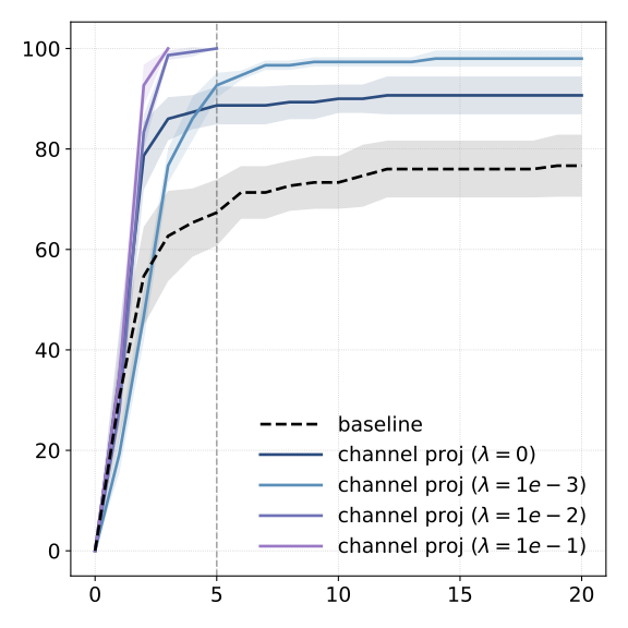
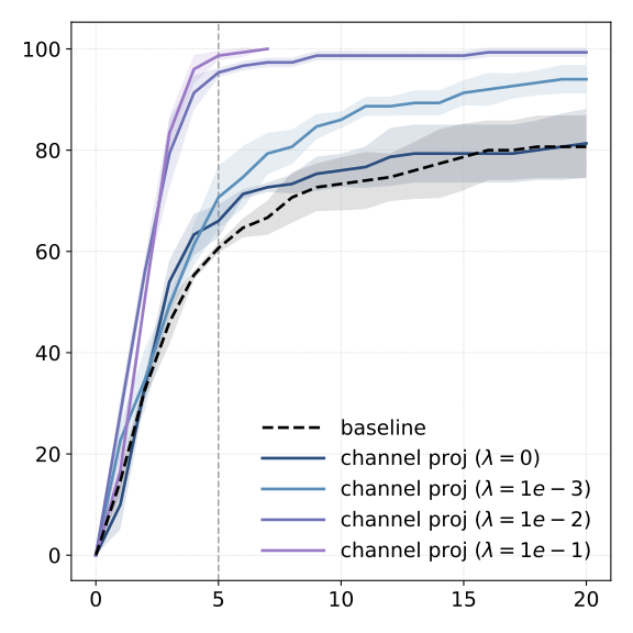
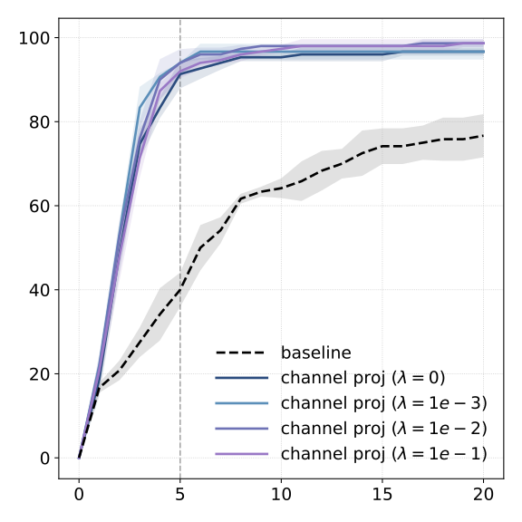
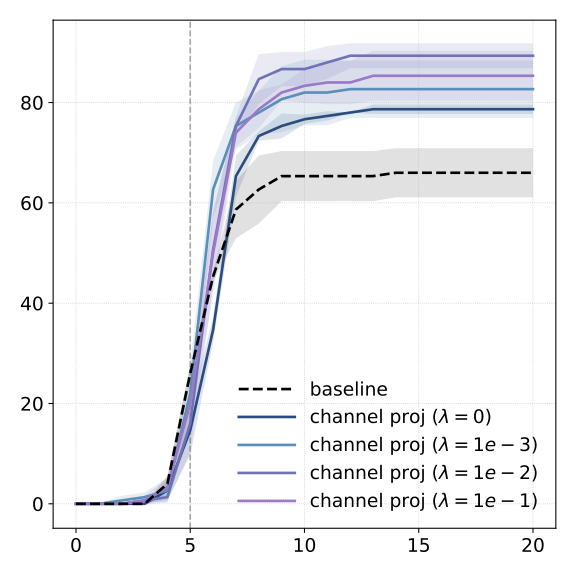
Learning a projector or encoder already improves several baselines, and explicit straightening often adds another gain. Reported perfect success on some easy MPC tasks is scoped to the selected goals and seeds. The original table retains cases where encoder choice or feature geometry remains poor.
(a) Success

(b) Failure

Comparison of CEM and GD.
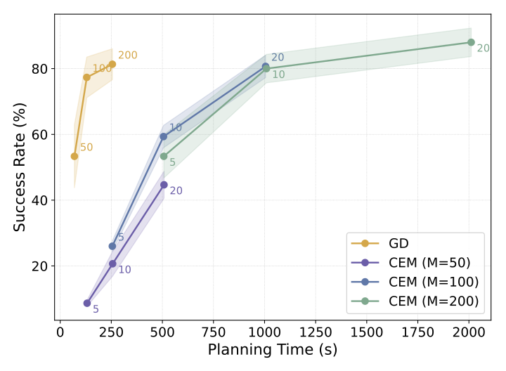
CEM often achieves higher absolute success but evaluates many more candidate rollouts. Straightening improves both planners and reduces the gap, producing a favorable gradient-planning latency tradeoff in the measured implementation.
Effect of feature dimensions.
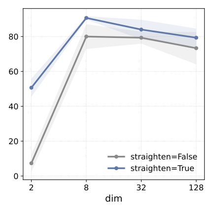
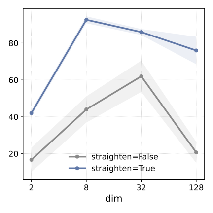
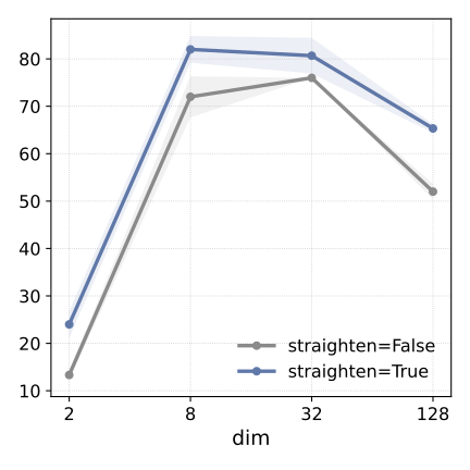
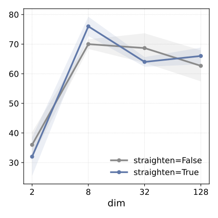
Keeping spatial tokens matters more than preserving every channel in these tasks. Moderate channel compression works well; two channels can be too few and very wide features can make planning harder. These are task-specific dimension ablations, not a universal optimal latent size.
Long horizon.
With goals fifty steps away, success drops and imagined trajectories can drift from the simulator. Adding an aggregated global goal cost to the spatial cost helps several long-horizon settings. Easier mazes are omitted from this test because a long random trajectory does not necessarily create a distant shortest-path goal.
Teleported-PointMaze.
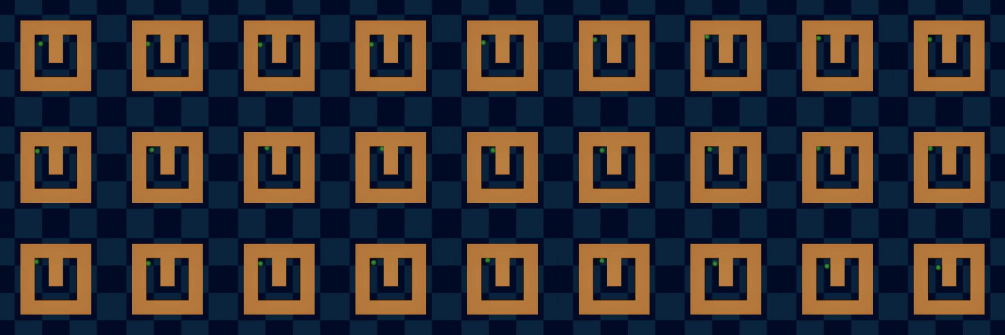
A modified maze teleports the agent from the right boundary to the left. A selected successful plan shows that learned temporal geometry can exploit a transition that is visually discontinuous. This is a diagnostic example, not a broad success-rate claim for all teleportation tasks.
Limitations and future directions.
The planner uses a symmetric Euclidean cost, which may be unsuitable for irreversible or asymmetric reachability. The local regularizer does not require reversibility, but directional costs may still be needed. Prediction features and the best planning-cost features can also be different spaces.
| Model | PushT | PointMaze – Medium | |||
|---|---|---|---|---|---|
| Open-loop | MPC | Open-loop | MPC | ||
| DINO-WM | – | 3.33 2.36 | 27.33 6.66 | 35.00 2.35 | 65.33 3.13 |
| + Proj | ✗ | 6.67 3.77 | 26.67 9.98 | 60.00 3.27 | 72.00 0.00 |
| + Proj | ✓ | 13.33 3.77 | 24.00 6.53 | 68.00 8.64 | 88.00 3.27 |
| ResNet | ✗ | 13.33 3.77 | 29.33 9.43 | 14.67 6.80 | 48.00 9.80 |
| ResNet | ✓ | 10.67 4.99 | 33.33 4.99 | 76.00 6.53 | 98.67 1.89 |
| Combined planning cost: | |||||
| + Proj | ✓ | 20.00 0.00 | 33.33 4.16 | 66.67 7.57 | 92.00 5.29 |
| ResNet | ✓ | 13.33 4.62 | 36.00 5.29 | 68.67 4.16 | 98.67 1.15 |
6 Conclusion
The contribution is a simple training-time geometric objective that improves several latent planners. Its strength is making action search easier without a new pixel generator or reward model. The remaining limits are learned-model error, task-dependent geometry and the gap between linear analysis and nonlinear deployment.
Impact Statement
The authors identify potential robotics and autonomous-system uses and call for attention to deployment safety. The experiments themselves remain simulated.
Acknowledgments
The source acknowledges research discussions, grants and computing support.
Appendix
Appendix A Data and Environments
A.1 Wall
Wall uses image-based two-room navigation with direct displacement actions. Its simple transitions differ from inertial physics in PointMaze.
A.2 PointMaze (UMaze and Medium-Maze)
The two PointMaze tasks use force inputs and include velocity and inertia. Separate datasets cover U-shaped and more complex layouts. These dynamics make short visual history important.
A.3 PushT
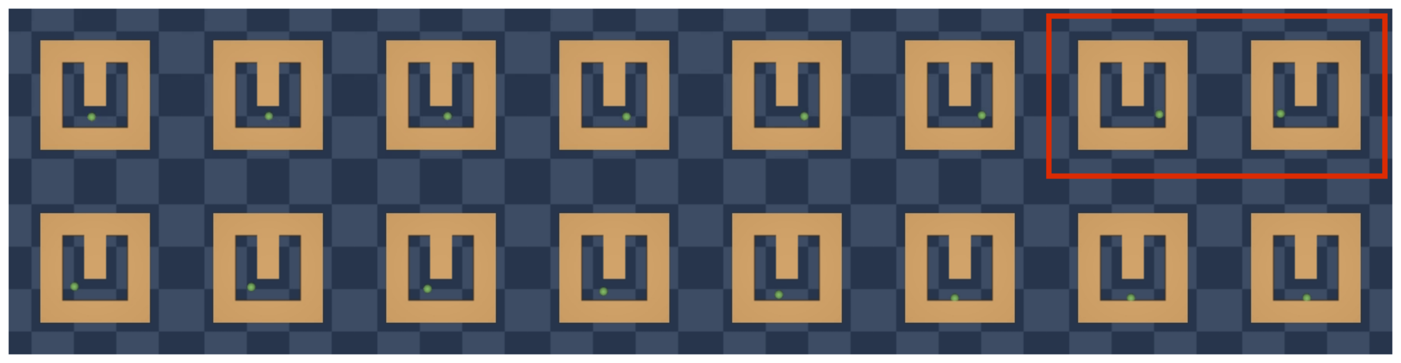
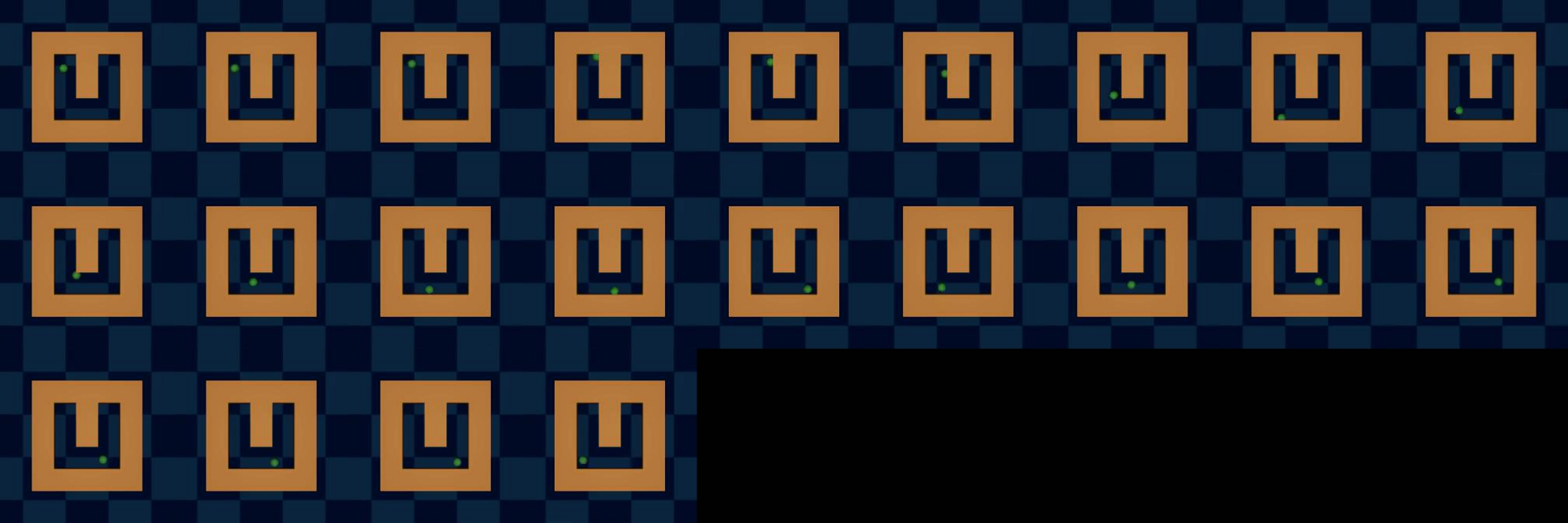
PushT requires both the pusher and T-block to match a feasible goal. The fixed green marker is a visual reference, not the target. Its reused dataset contains expert-derived noisy trajectories, so the evaluation is not uniformly based on random behavior.
Appendix B Experiments
B.1 Model Predictive Control (MPC)
Gradient descent differentiates goal error through an imagined rollout, updates the candidate actions, executes a prefix and replans from observed feedback. The main text adds task-specific intermediate losses beyond the simplified terminal-cost outline here.
Equations
B.2 Hyperparameters
The source tables retain training and planning hyperparameters. Reproduction requires matching encoder setup, feature shape, loss weight and action-chunk conventions.
| Name | Value |
|---|---|
| Spatial Projector/ResNet lr | 1e-522 2 We observe severe performance degradation when training without straightening and decreasing the learning rate helps. We thus use for no straightening. |
| Global Projector/ResNet lr | 1e-6 |
| Predictor lr | 5e-4 |
| Action/Prop encoder lr | 5e-4 |
| Batch size | 32 |
| History frames | 3 |
| Frameskip | 5 |
| Name | Value |
|---|---|
| Subplanner horizon | 25 |
| # Executed actions | 2533 3 This is for open-loop. If using MPC, we execute the first 5 actions (or the first chunk of actions if using a frameskip of 5). |
| Optimizer | Adam |
| Action Initialization | Zero |
| Learning rate | 0.1 |
| #opt steps | 100 |
B.3 Planning: GD vs. CEM
The timing comparison uses a single L40S and fifty PushT episodes. CEM’s candidate population provides more search effort, while gradient descent uses forward and backward passes on a proposed sequence. The observed speed ratio is an implementation-and-budget result, not a fixed complexity ratio for every device.
| Method | Config | Wall | PointMaze – UMaze | PointMaze – Medium | PushT | |||||
|---|---|---|---|---|---|---|---|---|---|---|
| dim | GD | CEM | GD | CEM | GD | CEM | GD | CEM | ||
| DINOv2 (patch) | ✗ | 52.67 5.73 | 87.33 4.99 | 35.33 4.11 | 88.00 1.63 | 40.83 10.07 | 88.00 1.63 | 56.00 4.32 | 71.33 7.72 | |
| DINOv2 (patch) + proj | ✗ | 80.00 7.12 | 92.00 0.00 | 44.00 7.12 | 75.33 4.99 | 72.00 4.32 | 92.67 4.71 | 70.00 1.63 | 71.33 6.18 | |
| DINOv2 (patch) + proj | ✓ | 90.67 0.94 | 100.00 0.00 | 94.00 1.63 | 94.00 1.63 | 82.67 3.77 | 86.67 1.89 | 77.33 6.18 | 80.00 4.32 | |
| ResNet | ✗ | 1.33 1.89 | 1.33 0.94 | 14.67 4.99 | 20.67 0.94 | 18.67 4.11 | 24.00 4.32 | 71.33 7.36 | 56.00 0.00 | |
| ResNet | ✓ | 84.67 2.49 | 90.00 5.89 | 64.67 8.38 | 83.33 2.49 | 80.67 0.94 | 89.33 6.18 | 70.67 0.94 | 72.67 6.60 | |
B.4 Effect of Feature Dimensions
Dimension ablations retain the full patch grid while reducing channels. The strongest results use moderate compression. They isolate channel count more directly than comparisons that also collapse the spatial grid.
B.5 Comparison to Smoothness and Temporal Contrastive Objectives
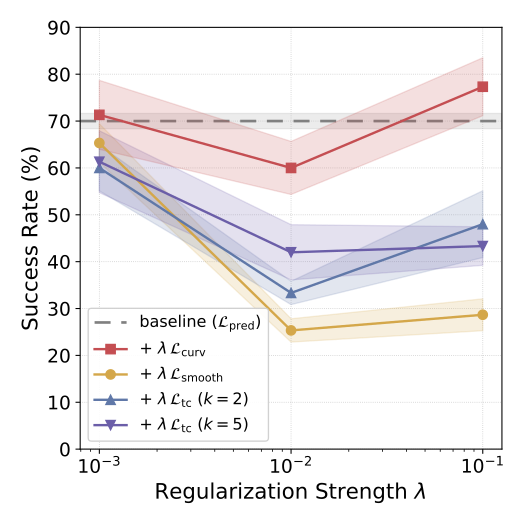
Smoothness shrinks adjacent latent distances; temporal contrastiveness separates distant-in-time observations. Neither matches straightening in this PushT comparison, and large weights can hurt. This does not show that either objective is useless in other settings.
Equations
B.6 Cosine Similarity Variants for Spatial Features
The aggregation head supplies a global trajectory direction while spatial features retain local detail for prediction. Its best reported regularization weight differs from those used for the other cosine variants, so the comparison includes that tuning choice.
Equations
Appendix C Theoretical Analysis
C.1 Setup and notation
The analysis defines linear dynamics and uses an effective condition number based only on nonzero singular values. This is necessary because many action sequences can produce the same terminal state, leaving a nullspace in the action Hessian.
Equation 14
| (14) |
Assumption C.1 (Linear latent dynamics).
We assume linear latent dynamics
Equation 15
| (15) |
Definition C.2 (Effective condition number).
For a PSD matrix with a nontrivial nullspace, define
Equation
where is the smallest nonzero singular value.
Definition C.3 (-straight transition).
In the linear model (15), define
Equation
C.2 Conditioning of the planning Hessian
Unrolling the linear system gives a terminal-state Jacobian built from successive transition powers and action matrices. Its Gramian shares nonzero eigenvalues with the action Hessian. This converts the optimization question into a standard reachability-conditioning question.
Equations 16–18
| (16) |
| (17) |
| (18) |
Lemma C.4 (Hessian form and Gramian equivalence).
Theorem C.5 (Conditioning bound).
Assume (15). Consider first the square-action case with invertible. Then
Equation 21
| (21) |
where . If additionally , then
Equation 22
| (22) |
Upper bound.
The upper bound combines the largest action gain with the largest transition gain at each horizon step. It limits how steep the strongest action direction can become.
Equations
Lower bound.
The lower bound depends on the action matrix being invertible, ensuring every state direction receives some action influence. This assumption cannot be silently applied to underactuated systems.
Equations
Combine.
Dividing the bounds controls the ratio of steepest to weakest nonzero directions. The expression also depends on action conditioning; straight transitions alone cannot repair an arbitrarily ill-conditioned action map.
Equation
ε -specialization.
Near-identity transitions bound their largest and smallest singular values, yielding the stated horizon-dependent estimate. For low-dimensional actions, extra controllability assumptions are needed to bound the smallest positive Gramian eigenvalue. Merely restricting to a reachable subspace does not supply that missing quantitative bound.
Remark C.6 (Low-dimensional actions ).
If , then is not invertible and may be singular. All statements hold on the controllable subspace by replacing with and interpreting as an effective condition number. In this case, additional controllability assumptions are needed to lower bound .
C.3 Cosine similarity as a proxy
The cosine connection assumes constant nonzero latent speed and bounded changes in actions. It bounds deviation from identity along visited movement directions. Turning that into a global spectral bound needs adequate directional coverage. Thus high cosine on training trajectories is evidence for a useful proxy, not an unconditional guarantee over all latent states.
Assumption C.7 (Constant velocity and smooth actions).
Define latent velocities . Assume there exists a constant such that
Equation
Assume action smoothness .
Definition C.8 (Cosine similarity).
For , define
Equation
Proposition C.9 (Cosine proxy small along visited directions).
Equations
Remark C.10 (Directional vs. spectral control).
Proposition C.9 bounds only along visited directions . Upgrading this to a uniform spectral bound requires an additional coverage condition so that visited directions span the latent space. This is not an unreasonable assumption since training trajectories are typically collected to be diverse. Under such regimes, maximizing cosine similarity provides a meaningful proxy for making close to in spectral norm.
Appendix D Related Work (Cont.)
Straightening is distinct from forcing all dynamics to be linear: even a linear rotation traces curved paths. It also differs from locally linear control and Koopman models. The method allows a nonlinear predictor while directly shaping observed trajectory geometry.
Appendix E Visualizations
E.1 Distance Heatmaps
The heatmaps compare learned goal distances with grid-search distances. Four-neighbor and eight-neighbor graphs imply different legal routes, so their reference maps differ. The plots illustrate local versus global geometry; their particular discretization is not the continuous system itself.









E.2 Visualization of Latent Trajectories
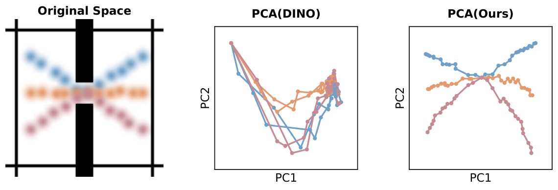
PCA plots make the change in trajectory geometry visible, while latent goal-error curves show whether distance tracks progress. A two-dimensional projection is illustrative and can hide structure in the remaining feature dimensions.










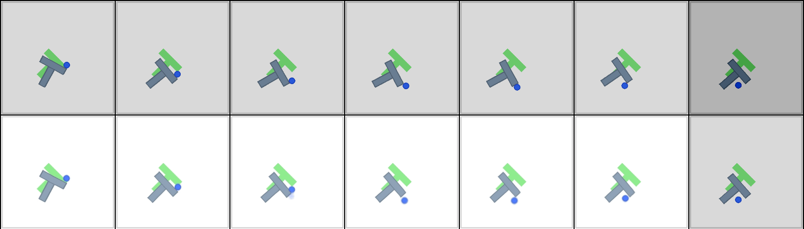
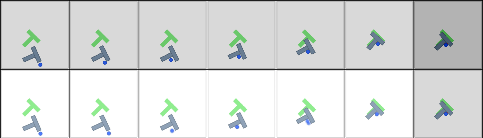
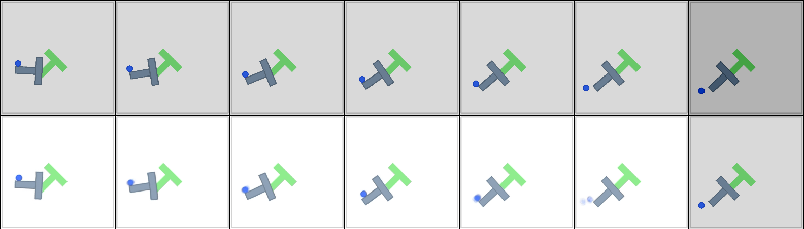
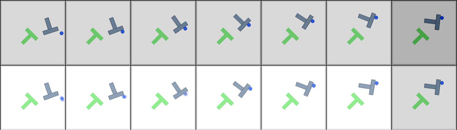
E.3 Planning Trajectories
The retained panels pair simulator execution with decoded imagined trajectories. Agreement and drift should be assessed separately; the latter reveals predictive-model failures that a low optimized latent cost can conceal.






Appendix F Teleported-PointMaze
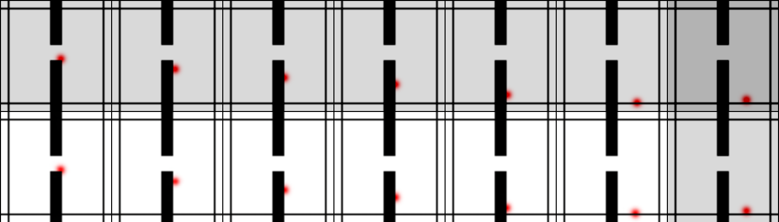
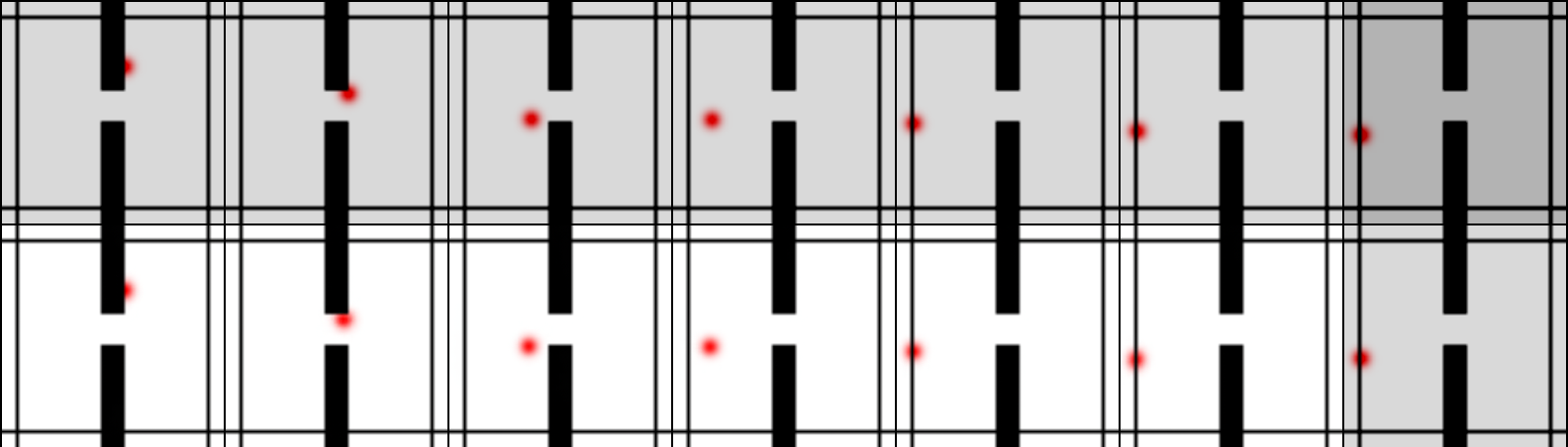
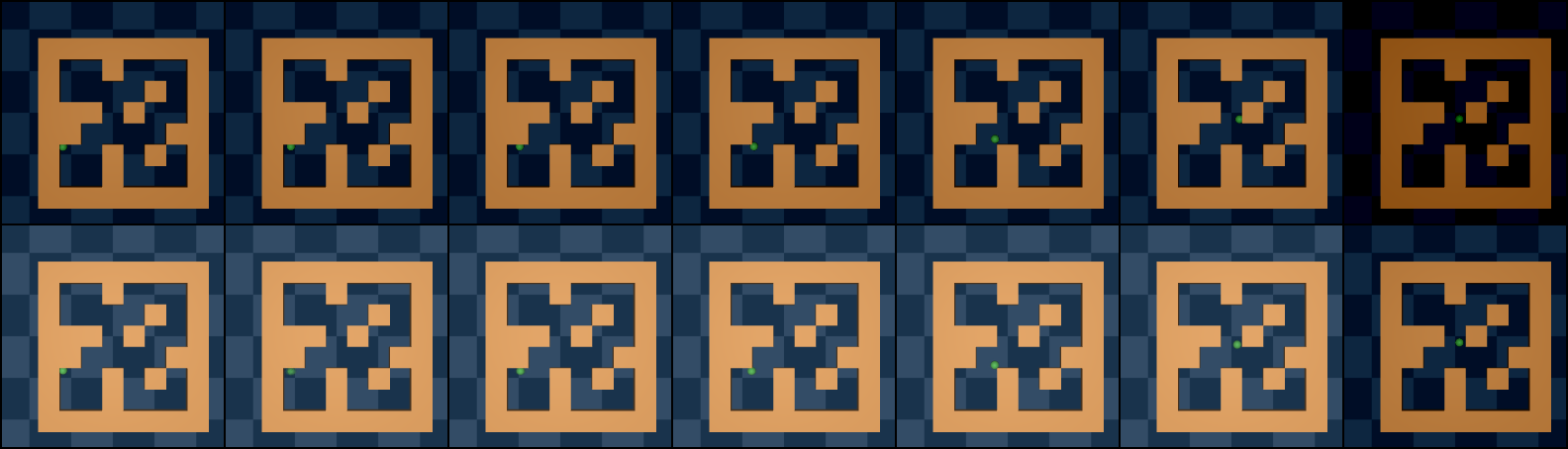
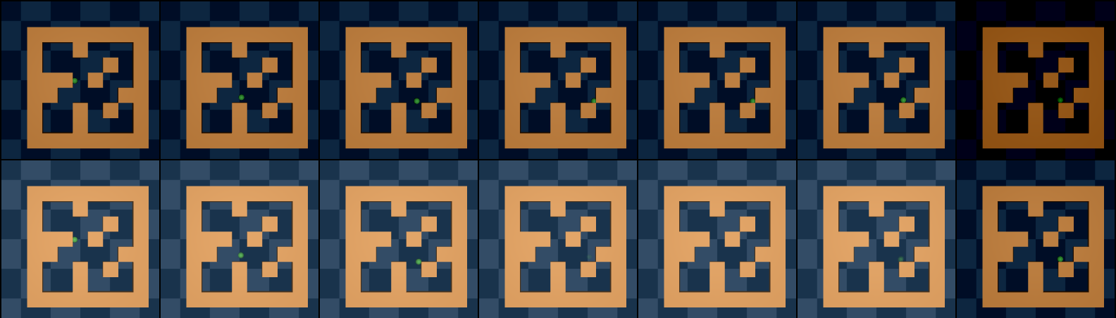
Teleportation changes position discontinuously and forces horizontal velocity to point right after the jump. This creates asymmetric temporal reachability. The example supports learning transition-sensitive geometry while reinforcing the limitation of using symmetric distance as a universal planning cost.