At a glance
FAKTUAL measures demonstration diversity through a signature kernel over whole trajectories, then chooses a smaller training set using entropy and determinant objectives. It needs neither a target policy nor online rollouts for selection.
Across simulated manipulation and four physical tasks, selected subsets often improve on random selection and sometimes on all available data. Results depend on task, budget, representation, and demonstration quality. This edition covers the complete 37-page revised paper, including Appendices A–I.
1. Introduction
Demonstration count hides redundancy, uneven behavior coverage, and differences in local density. A useful diversity measure must compare variable-length sequences of states, actions, and visual observations without reducing everything to independent frames.
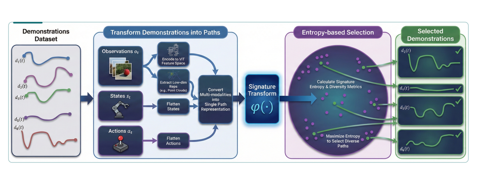
The paper adapts kernel-spectrum entropy, closely related to the Vendi score, to trajectory signatures. Diversity complements quality and sufficient nearby examples; it is not itself a success or quality score [1] [16] [17]. Figure 1 preserves the pipeline.
2. Signature transform and kernel
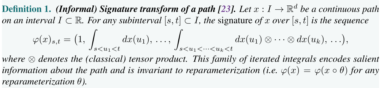
A path signature collects iterated integrals that encode sequential geometry. A signature kernel compares those representations without necessarily constructing their full, infinite tensors. Definitions 1 and 2 remain unchanged below.
Truncation, dynamic programming, random features, and a differential-equation formulation offer different computational trade-offs [23] [24] [25]. Reparameterization invariance can remove speed variation, but signatures also have translation and tree-like ambiguities; the appendix discussion needs those qualifications.

3. Problem statement
The setting is behavior cloning from successful state–action–observation trajectories. The retained objective averages loss within each demonstration and then across demonstrations, so unequal trajectory lengths do not automatically determine example weights.
The goal is a dataset-only statistic associated with closed-loop policy success and useful for subset selection. Similar entropy does not establish equivalent policy performance; that connection is assessed empirically, not proved.
Equation

4. Measuring diversity
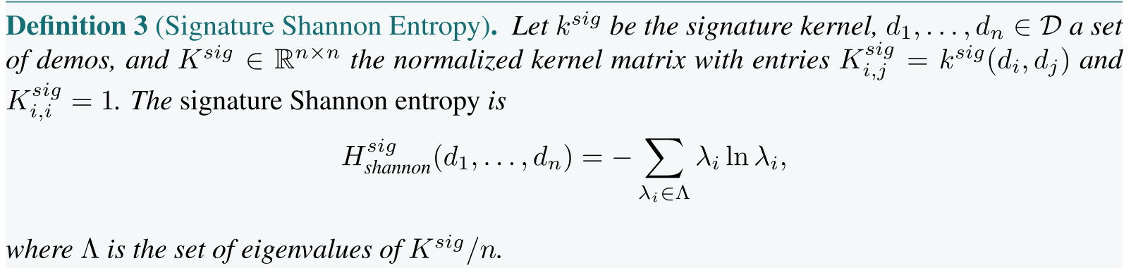
Normalize the signature Gram matrix to unit diagonal, divide by the number of demonstrations, and compute entropy from its nonnegative eigenvalues. They sum to one. The spectral Shannon entropy equals the matrix von Neumann entropy; exponentiating gives an effective rank/Vendi score [1] [30].
A second objective uses the Gram determinant to reward linearly independent feature directions. Geometrically, a Gram determinant is squared volume; the source calls it volume. Its behavior depends on the chosen kernel and representation, and unit-diagonal normalization alone does not ensure every widely separated pair has near-zero similarity.

5. Data curation
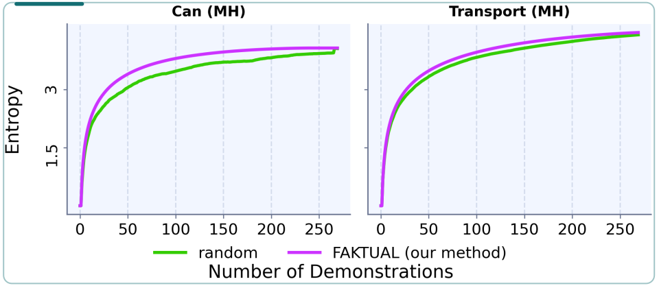
Given a budget m, approximate the entropy-maximizing subset with greedy-style selection. Observed entropy saturation suggests redundancy in some datasets; Figure 2 shows rapid saturation for Can and little saturation for Transport over the tested range.
An optional mixture first selects roughly a fraction p of the budget by entropy, then selects the remainder from unused demonstrations by determinant. The authors report useful p values between 0.5 and 0.9, while determinant-only selection can also work. Appendix F preserves the alternative solvers and their conditional guarantees.

6. Experiments and results
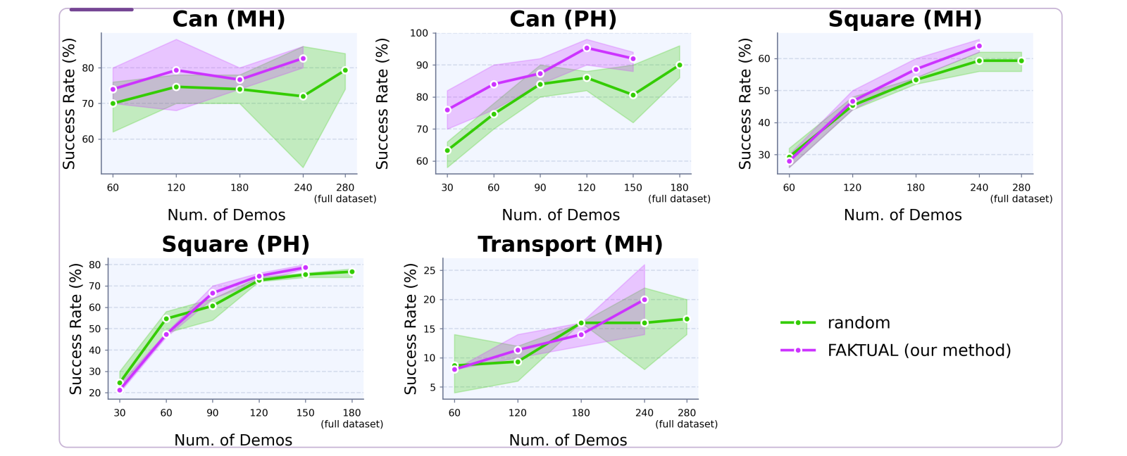
Experiments vary the demonstration budget, compare selection methods, and relate entropy to policy success. The plots generally report each seed’s maximum success across 20 evaluated checkpoints, followed by averaging across three seeds. Those are selected-checkpoint results, not final-checkpoint performance or confidence intervals.
6.1 Simulated experiments
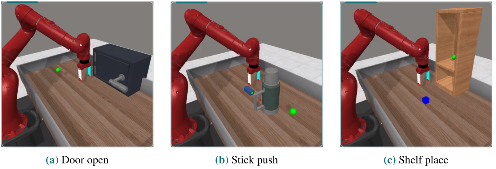
RoboMimic uses Can and Square with proficient-human and multi-human datasets, plus multi-human Transport. Can uses recurrent behavior cloning; Square and Transport use diffusion policies. MetaWorld fine-tunes SmolVLA on Door Open, Stick Push, and Shelf Place [16] [33] [38] [39].
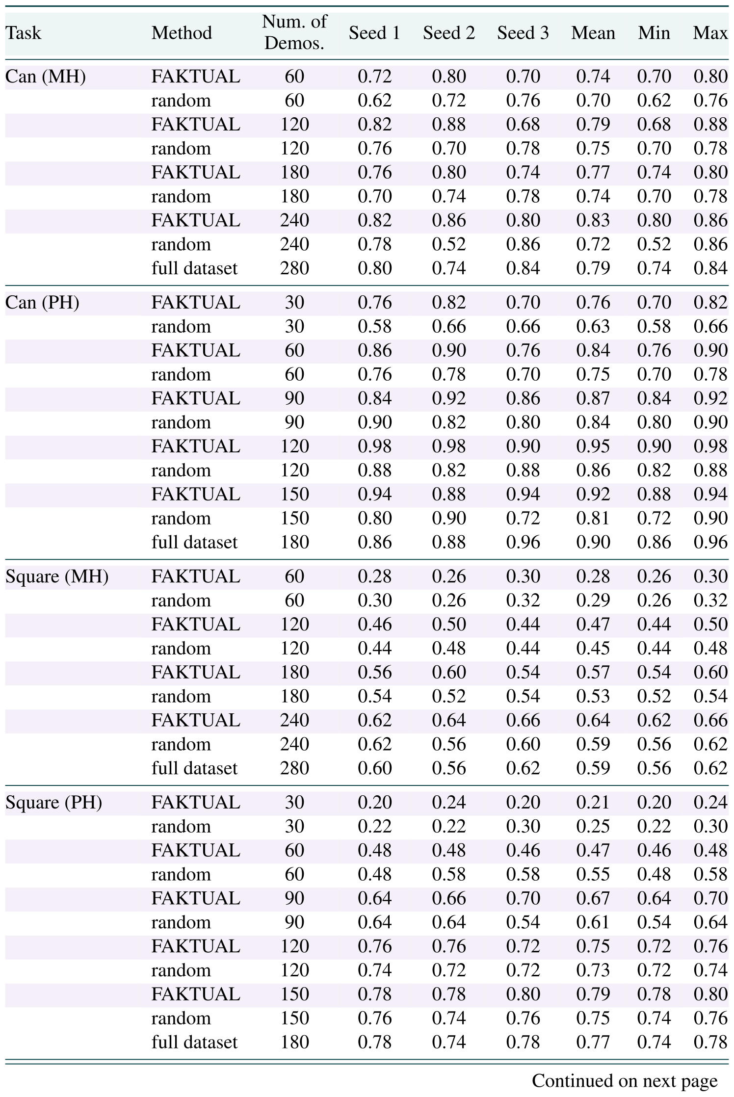
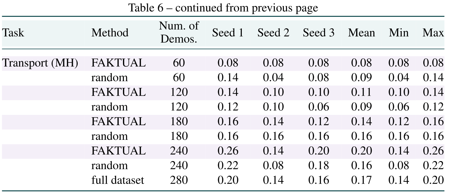
Can shows a clearer advantage than the harder tasks. Table 6 reports Can PH at 120 demonstrations as 0.95 versus 0.86 for random, but Square PH at 60 demonstrations as 0.47 versus 0.55. Transport MH at 180 demonstrations is also lower, 0.14 versus 0.16.
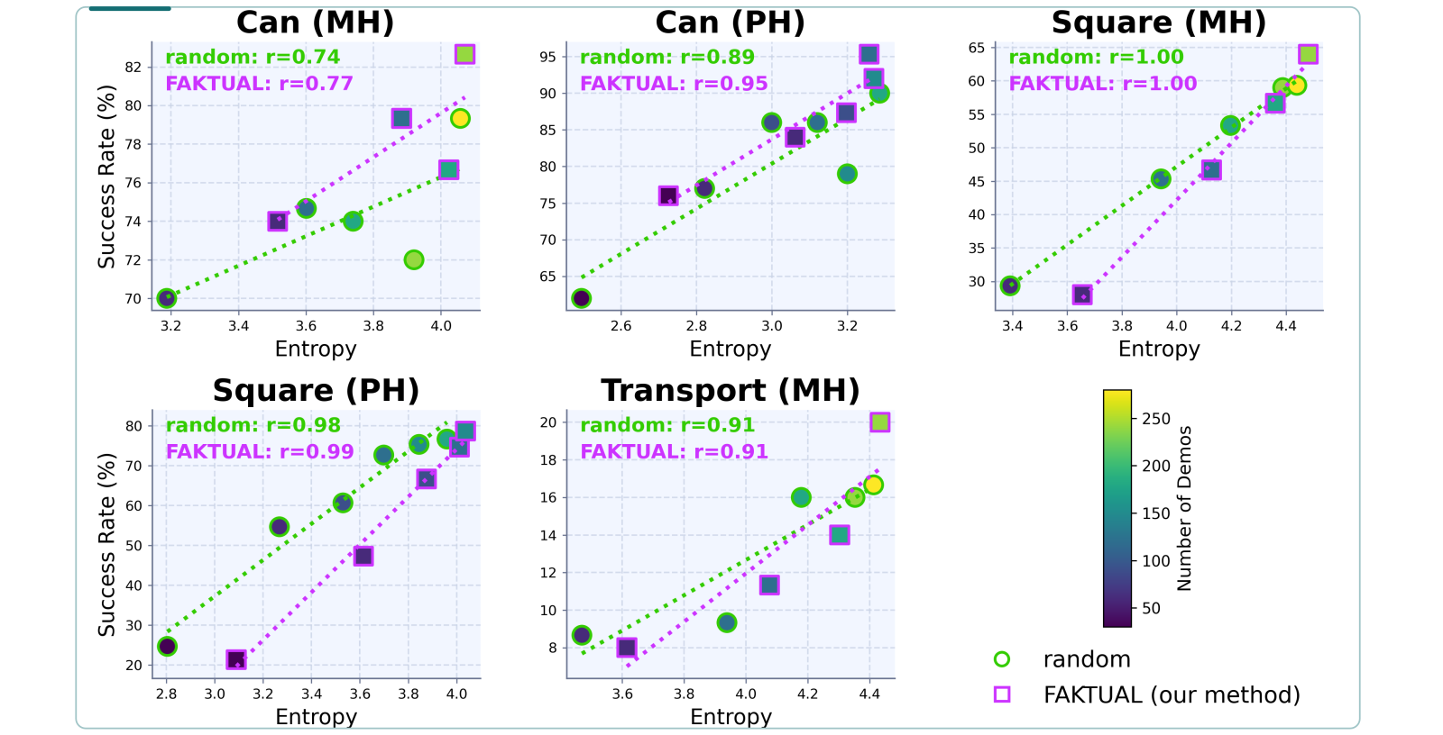
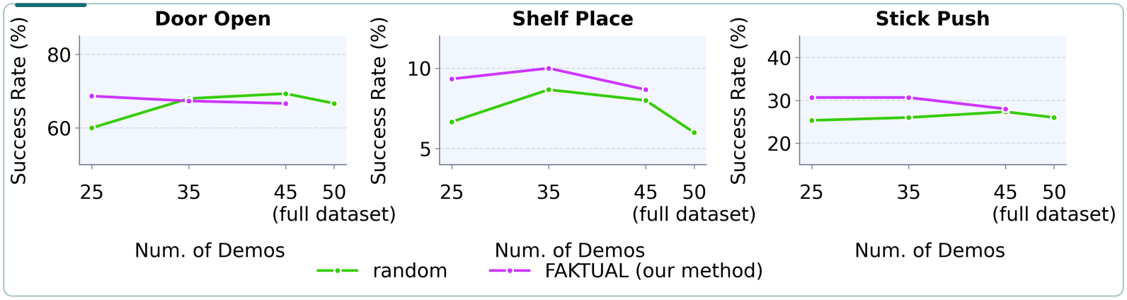
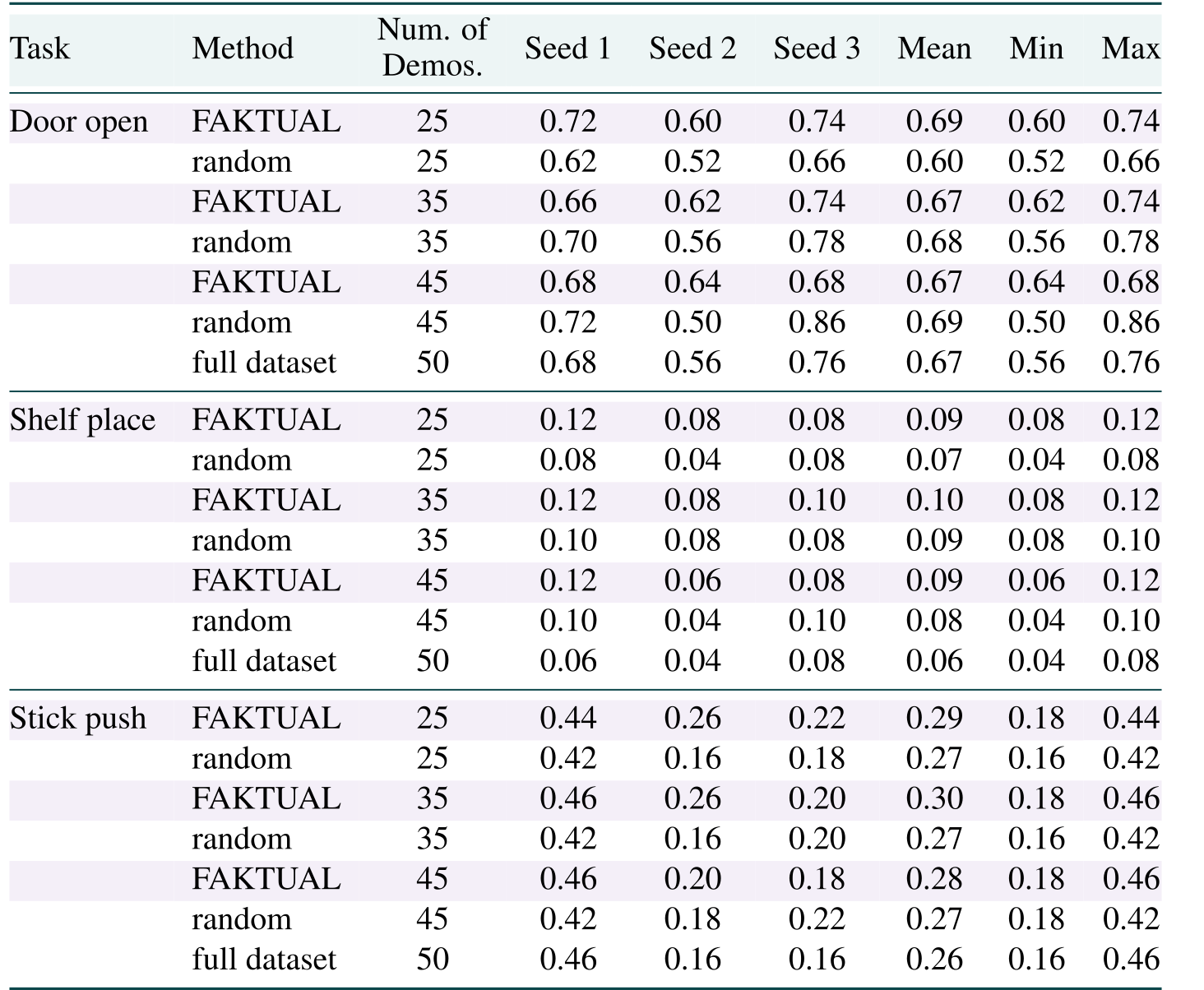
Figure 4 reports Pearson correlations of 0.74–1.00 between entropy and success. The plotted subsets also vary in size, so this association does not isolate a causal effect of diversity at fixed budget. MetaWorld gains are mixed: Door Open is slightly worse than random at budgets 35 and 45, while Shelf Place remains low for every method.
6.2 Real-world experiments
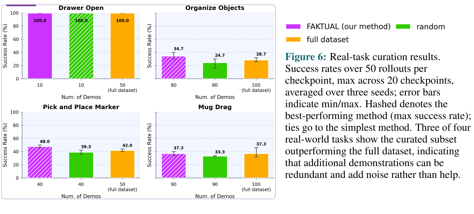
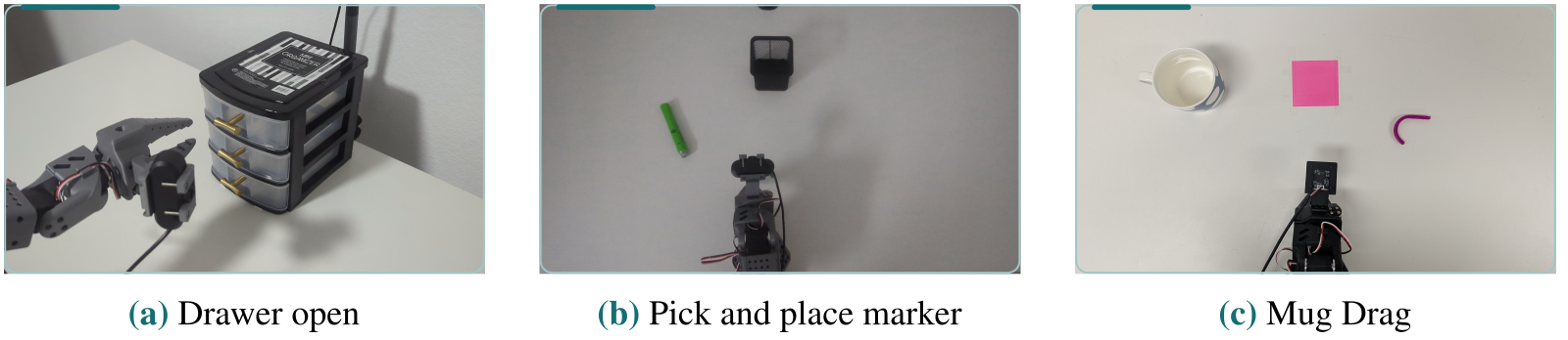
The SO-ARM101 experiments cover drawer opening, placing a marker in a holder, dragging a mug with a hook, and conditionally organizing a marker or charging brick. SmolVLA is used throughout. Figure 6 retains every panel and the complete original caption.
The Figure 6 caption claims improvements over all data on three tasks, but its printed bars show strict gains on two: organization (34.7% versus 28.7%) and marker placement (48.0% versus 42.0%). Drawer opening ties at 100%, and mug dragging ties at 37.3%. The original caption remains intact. These four laboratory tasks do not establish robustness to pathological data or broad deployment generalization. Appendix G records a separate checkpoint-schedule conflict.
6.3 Baselines
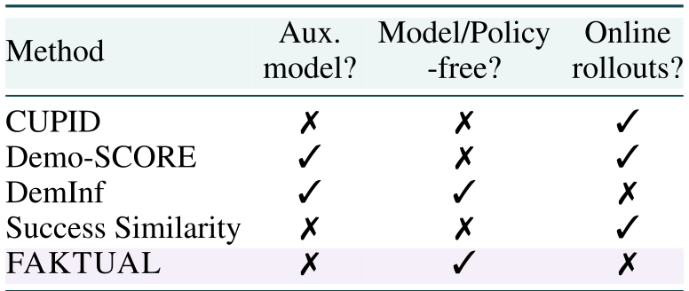
Comparisons include DemInf, CUPID, Demo-SCORE, an oracle with privileged labels, Success Similarity, and random selection [19] [22] [21]. Table 1 distinguishes auxiliary models, policy dependence, and online rollouts.
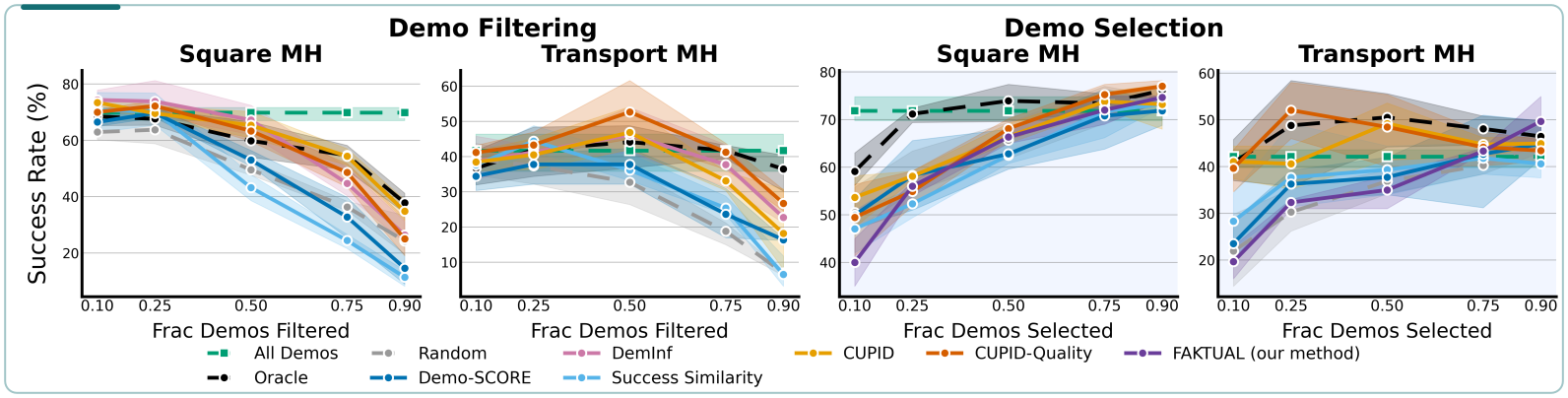
FAKTUAL generally beats random but remains below several stronger quality- or rollout-informed baselines in Figure 7. Its appeal is lower selection overhead. “Model-free” here means no learned scoring model or target-policy dependence; visual representations may still use a pretrained ViT.
Figure 7 uses low-dimensional observations instead of the ViT representations used elsewhere. Its absolute success rates therefore should not be directly compared with the earlier image-based experiment. The paper distinguishes selecting a subset from filtering low-quality demonstrations.
6.4 Observations
Diversity can hurt at small budgets when hard tasks need many nearby examples. The authors interpret the crossover as a balance between coverage and local density; they do not prove that entropy alone determines that balance.
Selection reduces the marker-location imbalance in one task. It fails to distinguish five drawer-lighting conditions and does not systematically prefer one object-organization goal. These observations show that the representation decides which forms of diversity are visible.
7. Ablations
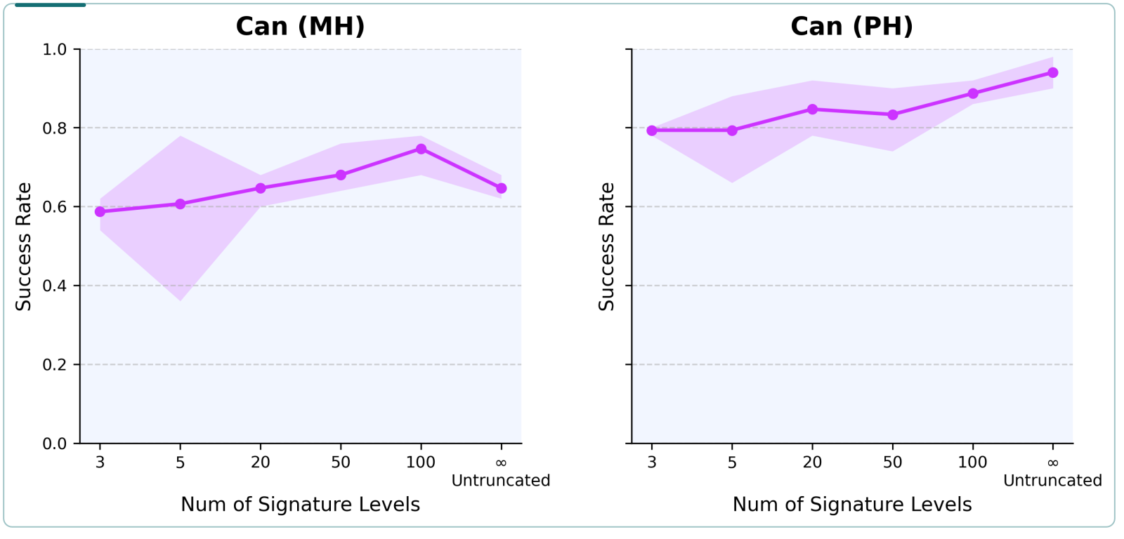
Increasing signature depth can help or hurt: fine trajectory detail may carry useful information or noise. Figure 12 varies signature levels, with budget m=120 and p=0; the main text’s phrase “improves with size m” does not match that fixed-budget plot.
The source reports useful entropy/determinant mixing across p=0.5–0.9 and says a global-alignment-kernel alternative performs like random. It provides no comparable detailed plot for those two claims.
8. Conclusion and limitations
FAKTUAL offers a policy-independent way to select less redundant demonstrations. The evidence supports a useful heuristic on the tested datasets, with quality-aware methods often stronger and low-budget diversity sometimes harmful.
All demonstrations are successful; adversarial or highly unusual harmful trajectories were not tested. The entropy–performance association is not causal, and there is no theory explaining saturation, the optimal subset size, or post-saturation degradation. Combining quality, balanced coverage, and local density remains a proposal.
B. Demonstrations as paths
Appendix B describes three ways to represent demonstrations. Their choices of modalities, visual encoder, normalization, camera, and temporal sampling affect the measured diversity.
B.1 Flatten and stack
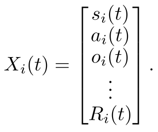
Embed each image with a fixed ViT or extract a low-dimensional observation, then concatenate it with states, actions, rewards, and other per-step features. The retained vector gives the exact construction. Full trajectories can have different lengths.
Equation
B.2 Combine modality kernels
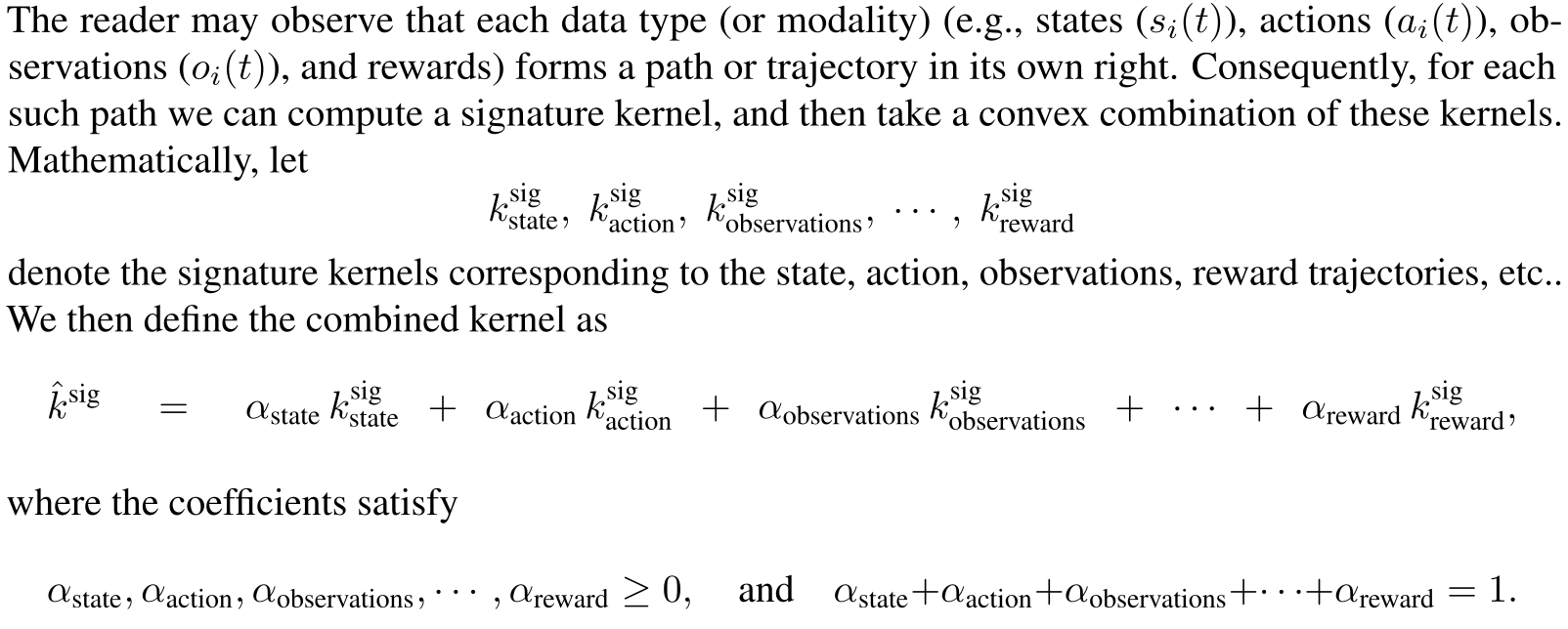
Alternatively compute a separate signature kernel for each modality and combine them with nonnegative weights summing to one. This preserves positive semidefiniteness and allows modality-specific hyperparameters. The authors report no improvement over stacking in their experiments.
Equation
B.3 Initial observation and motion
A cheaper variant mixes an RBF kernel on the initial visual observation with a signature kernel on the end-effector path. It separates initial scene diversity from motion diversity, but can miss distractors or scene changes that occur later.
Equations


B.4 Implementation practices
Temporal subsampling reduces work but can miss short-lived changes. The authors recommend one camera covering the whole scene and warn that wrist-camera motion can inflate apparent diversity. This curation recommendation is distinct from the multi-camera policy inputs used in the real tasks.
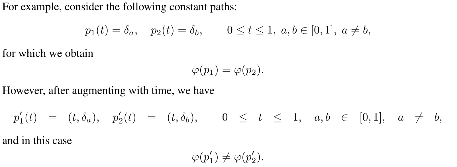
The original time-augmentation example is preserved below, but its conclusion is incorrect for the stated plain path signature: (t,a) and (t,b) differ by a constant translation and still have identical increments and signatures. Keeping starting-point information requires an additional construction, such as basepoint augmentation; see the cited primer [13]. Time augmentation alone addresses a different invariance.
Equation
C.1 Entropy
Shannon entropy averages the negative log probability of outcomes. Here the probability vector is supplied by the normalized kernel spectrum rather than a fitted distribution over demonstrations. Equation 2 is retained.
Equation

C.1.1 Von Neumann entropy
The matrix analogue is minus the trace of a unit-trace positive semidefinite matrix times its matrix logarithm. Its spectral form connects directly to Shannon entropy. Zero eigenvalues use the limiting convention 0 log 0=0.
Equation

C.2 Submodularity
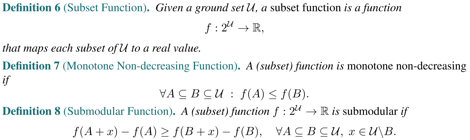
Definitions 6–8 retain set functions, monotonicity, and diminishing marginal returns. Later approximation ratios require these properties; empirical saturation by itself is not a proof that the normalized spectral-entropy objective is monotone and submodular.
D.1 Signature transform
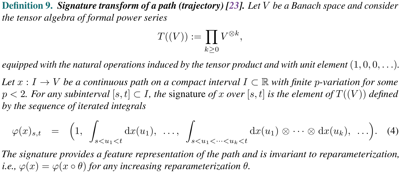
Definition 9 retains the tensor algebra and iterated-integral construction for continuous paths with finite variation assumptions. The original mathematical statements remain available for inspection.
D.1.1 Properties
Reversing a path gives its tensor inverse. Uniqueness must account for translation, time reparameterization, and tree-like equivalence; the source’s simple claim of injectivity for “non-tree-like paths” omits these qualifications [13].
Equation

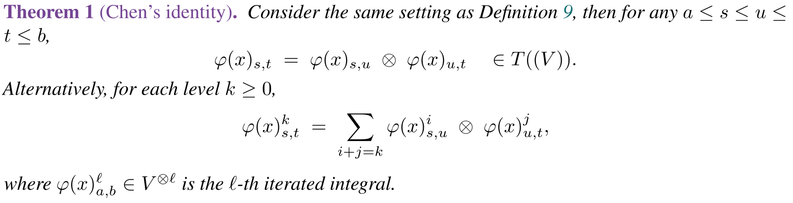
Chen’s identity
Chen’s identity composes successive path segments through tensor multiplication. The retained theorem includes both the whole-signature and levelwise forms, followed by the group-like coproduct relation.
Equation

Truncation
Finite truncation reduces the feature representation to finitely many tensor levels. The original decay bound and Equation 5 remain below. The stated general p-variation factorial bound should be checked against the cited rough-path source before using it as a numerical error guarantee; the paper does not derive it [29].
Equations


D.2 Signature kernel
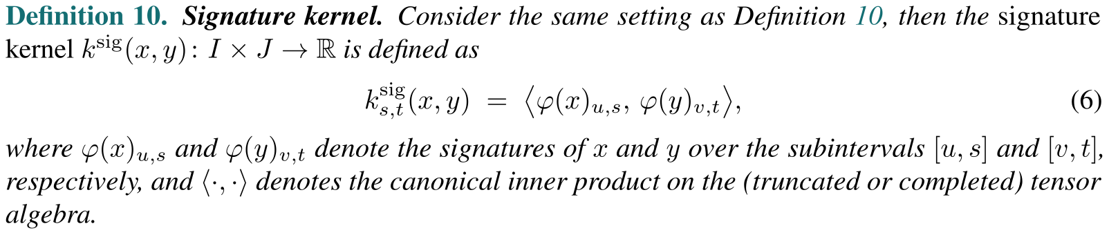
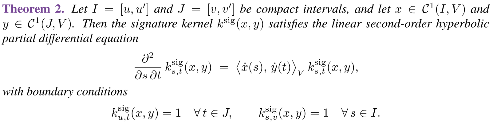
Definition 10 takes an inner product between signatures. Theorem 2 expresses the untruncated kernel for differentiable paths as a second-order hyperbolic PDE with unit boundary values [23].
Pairwise kernel evaluation and forming an entire dataset Gram matrix are different costs. The latter still requires quadratically many pairs. The source’s effectively linear per-pair GPU wall time assumes sufficient parallel hardware and does not make the full dataset calculation linear.
E. Random Fourier signature features
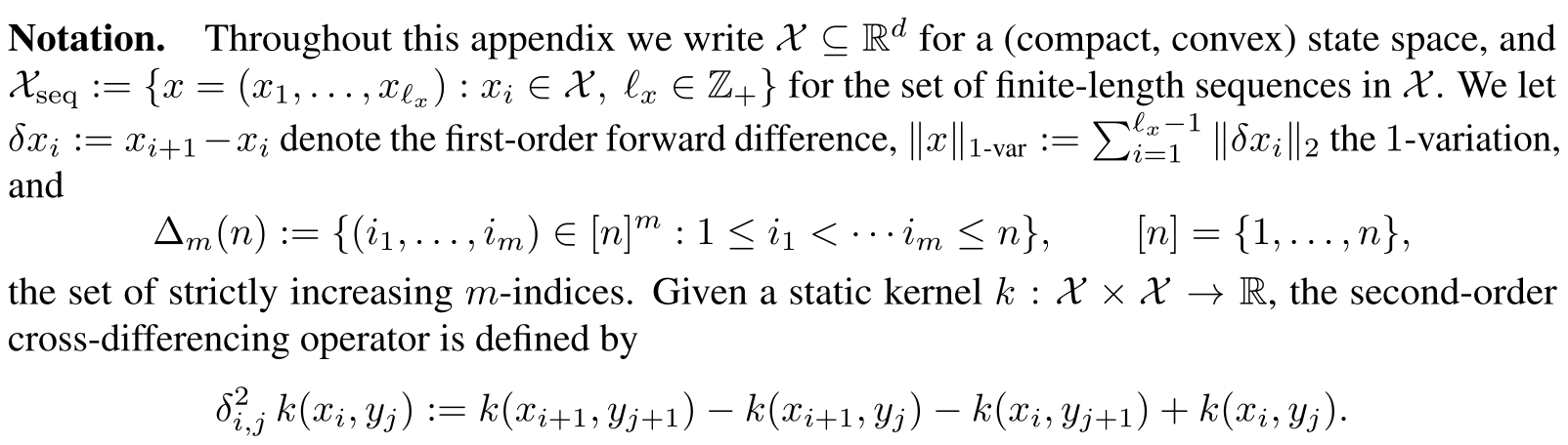
Appendix E presents random Fourier signature features from Tóth and colleagues [25]. It fixes sequence increments, ordered index sets, bounded variation, and a static kernel, then gives the discrete truncated expansion in Equation 7.
Random features reduce the per-sequence representation cost. Forming and repeatedly processing a dense Gram matrix can still dominate large-dataset curation; the paper supplies no end-to-end timing table establishing negligible overhead at arbitrary scale.
Equations

E.1 Random Fourier features
A translation-invariant kernel can be approximated by sine/cosine features sampled from its spectral measure. Gaussian kernels use Gaussian spectral weights. The original Fourier map and moment assumption in Equation 8 remain unchanged.
Equations



E.2 Signature features
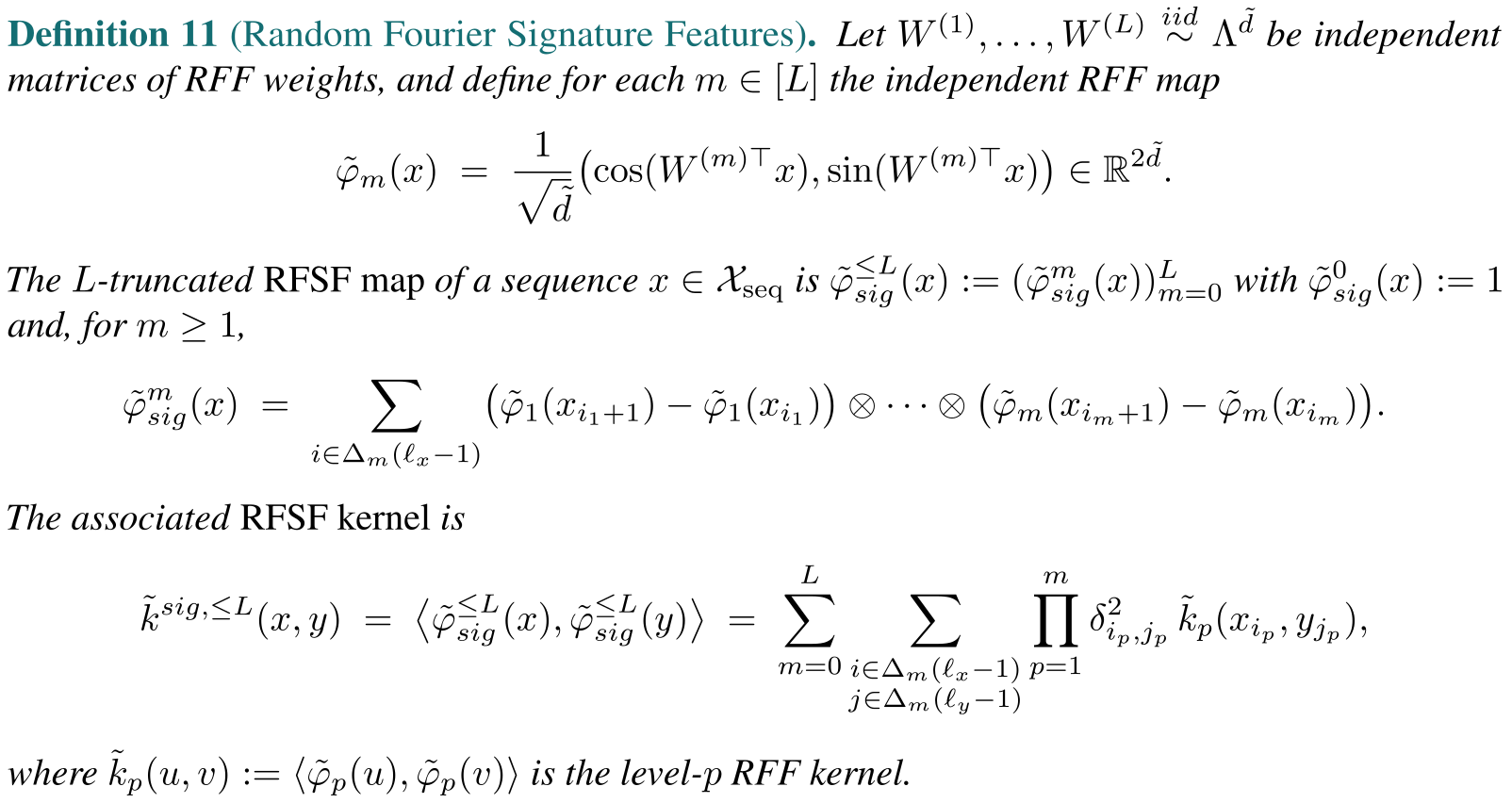
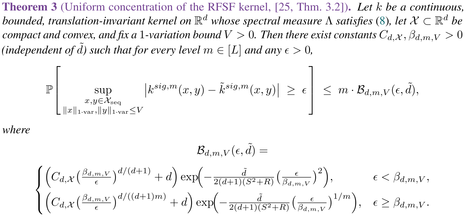
Independent random-feature realizations across tensor levels avoid the bias of a naive shared-feature construction. Definition 11 gives the complete map and kernel; Theorem 3 gives concentration under compact-domain, variation, and moment assumptions.
The theorem concerns kernel approximation, not policy success or a guaranteed optimal curated set. Explicit tensor features grow rapidly with feature dimension and truncation depth, motivating the two projections below.
E.3 Diagonal projection
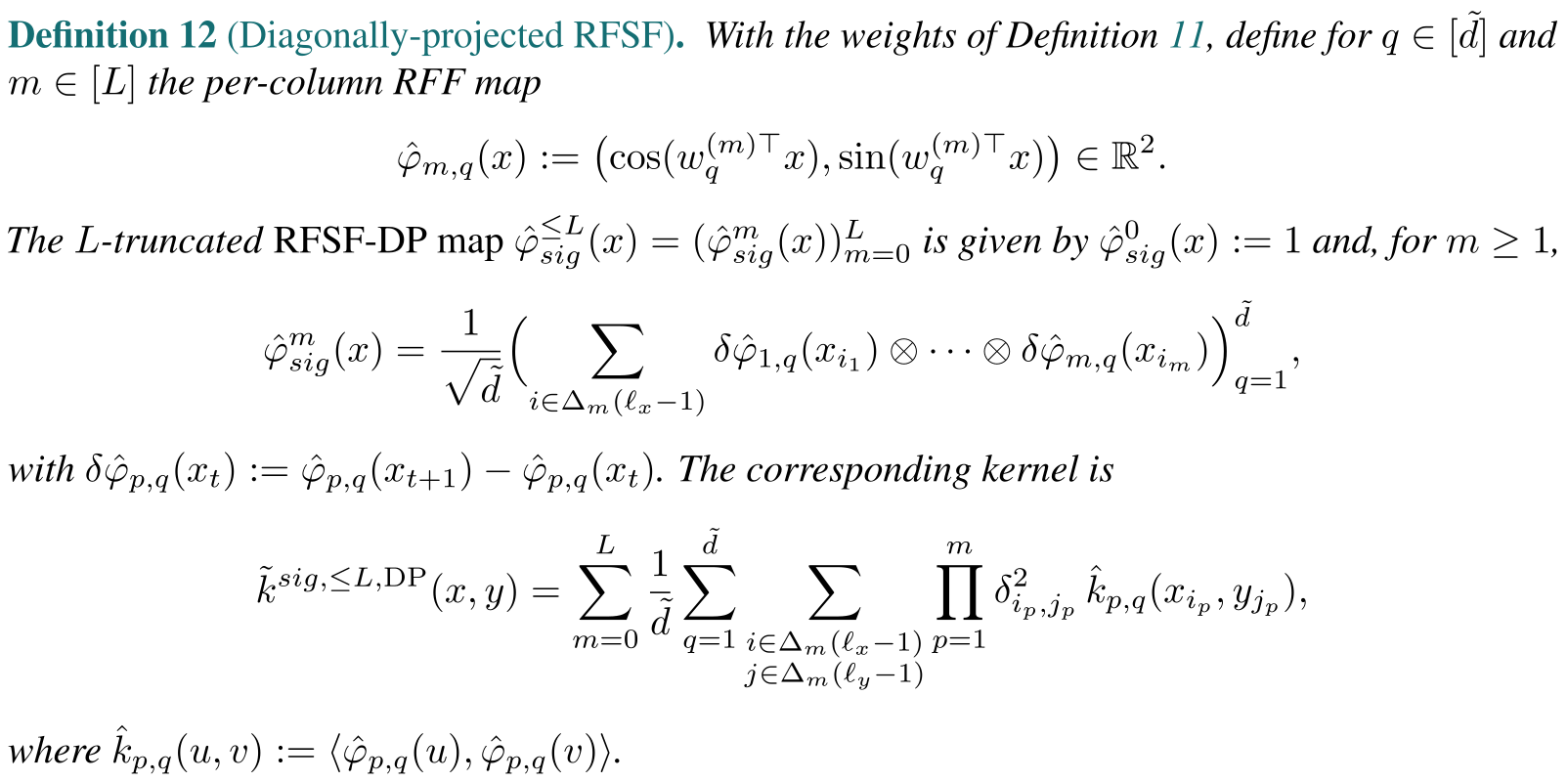
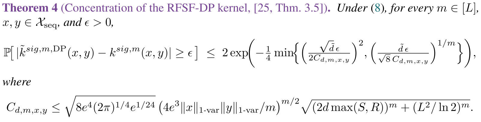
RFSF-DP restricts the outer feature-index sum to diagonal combinations. It remains unbiased while reducing feature dimension to linear dependence on random-feature width, with exponential dependence on signature depth. Definition 12, Theorem 4, and the stated computational cost are preserved.
Equations

E.4 Tensor random projection
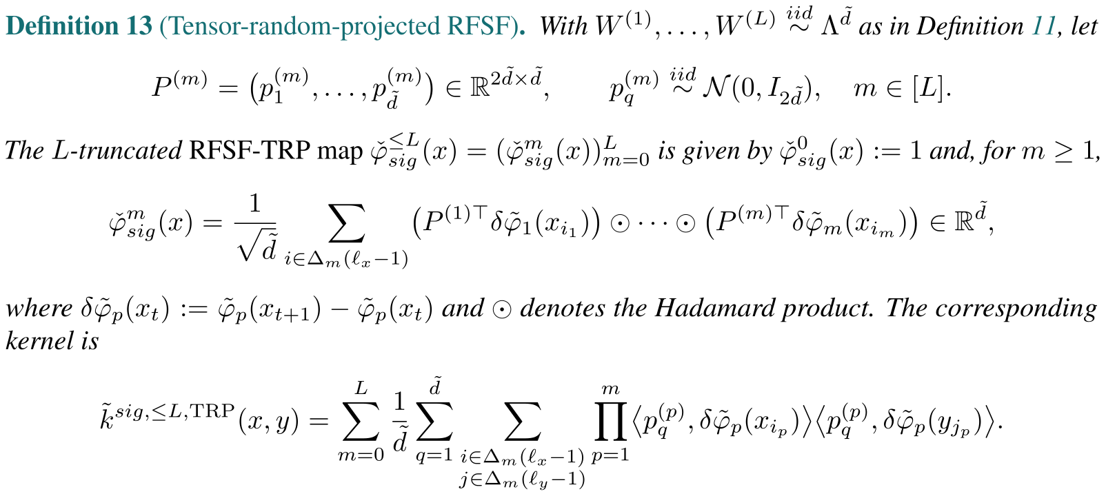
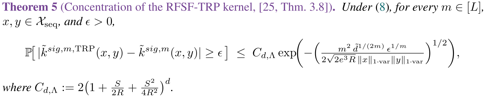
RFSF-TRP projects tensor products to lower dimension and evaluates them through Hadamard products without materializing full tensors. Definition 13 and Theorem 5 retain the construction and its concentration bound; approximation to the true kernel additionally uses the earlier random-feature bound.
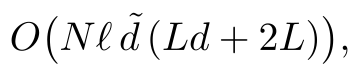
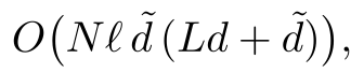
The reported cost is linear in sequence length but contains a quadratic term in feature width. It should not be described as strictly linear in every dimension.
Equation
E.5 Computational trade-offs
Table 2 preserves feature dimensions, per-sequence costs, and concentration rates. The last paragraph names a DP empirical kernel but calls the ablation implementation TRP; that notation mismatch is retained and should be resolved against implementation before reproduction.
Entrywise kernel approximation does not by itself establish accuracy of entropy, determinant rankings, or downstream policy performance without further stability analysis.

F. Subset algorithms
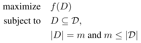
Appendix F formulates fixed-budget subset optimization and introduces a regularized log determinant for numerical stability. Its claim that adding μI leaves the optimizer unchanged is not generally justified: a log transform preserves determinant rankings, but diagonal regularization can change them.
Exact search is proposed for small datasets; greedy, stochastic, and determinantal sampling are alternatives for larger ones. The text invokes maximum coverage and integer-programming hardness without giving a reduction specific to each stated objective.
Equations

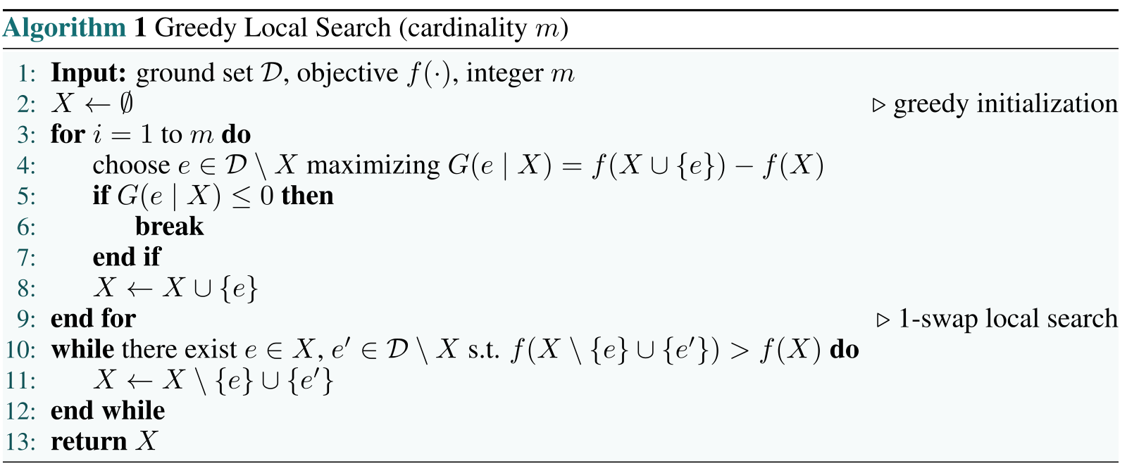
F.1 Greedy local search
Algorithm 1 greedily adds the greatest marginal gain and optionally performs improving single-element swaps. It stops early when the best gain is nonpositive, so its printed code can return fewer than m elements.
The familiar 1−1/e guarantee is conditional on a nonnegative monotone submodular objective under a cardinality upper bound. It is not an unconditional guarantee for FAKTUAL’s normalized entropy objective [75] [76].
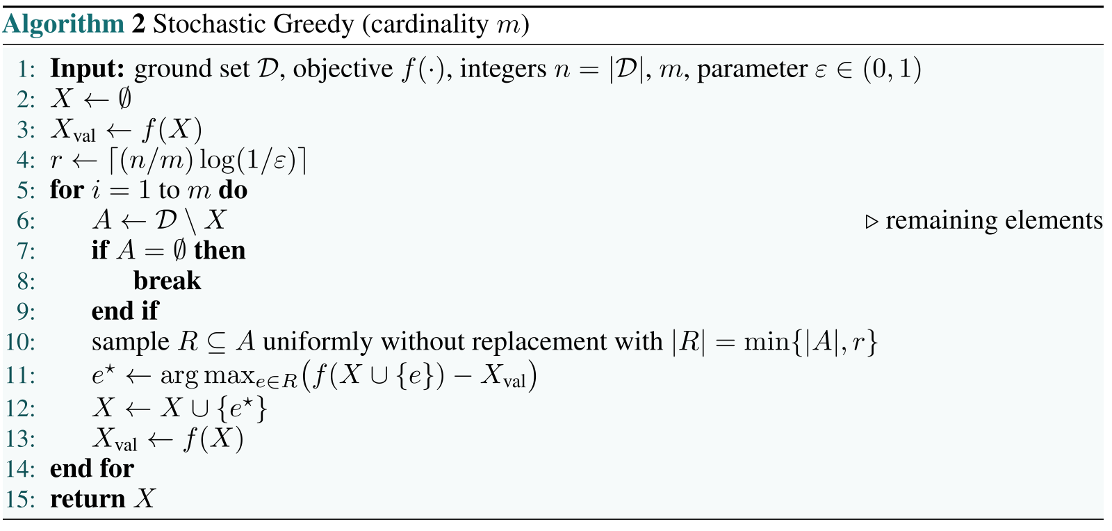
F.2 Stochastic greedy
Algorithm 2 evaluates gains only within a fresh random candidate subset at each iteration. The stated expected approximation factor is 1−1/e−ε under the same objective assumptions; its reduced function-evaluation count does not include the cost of each entropy or determinant evaluation [77].
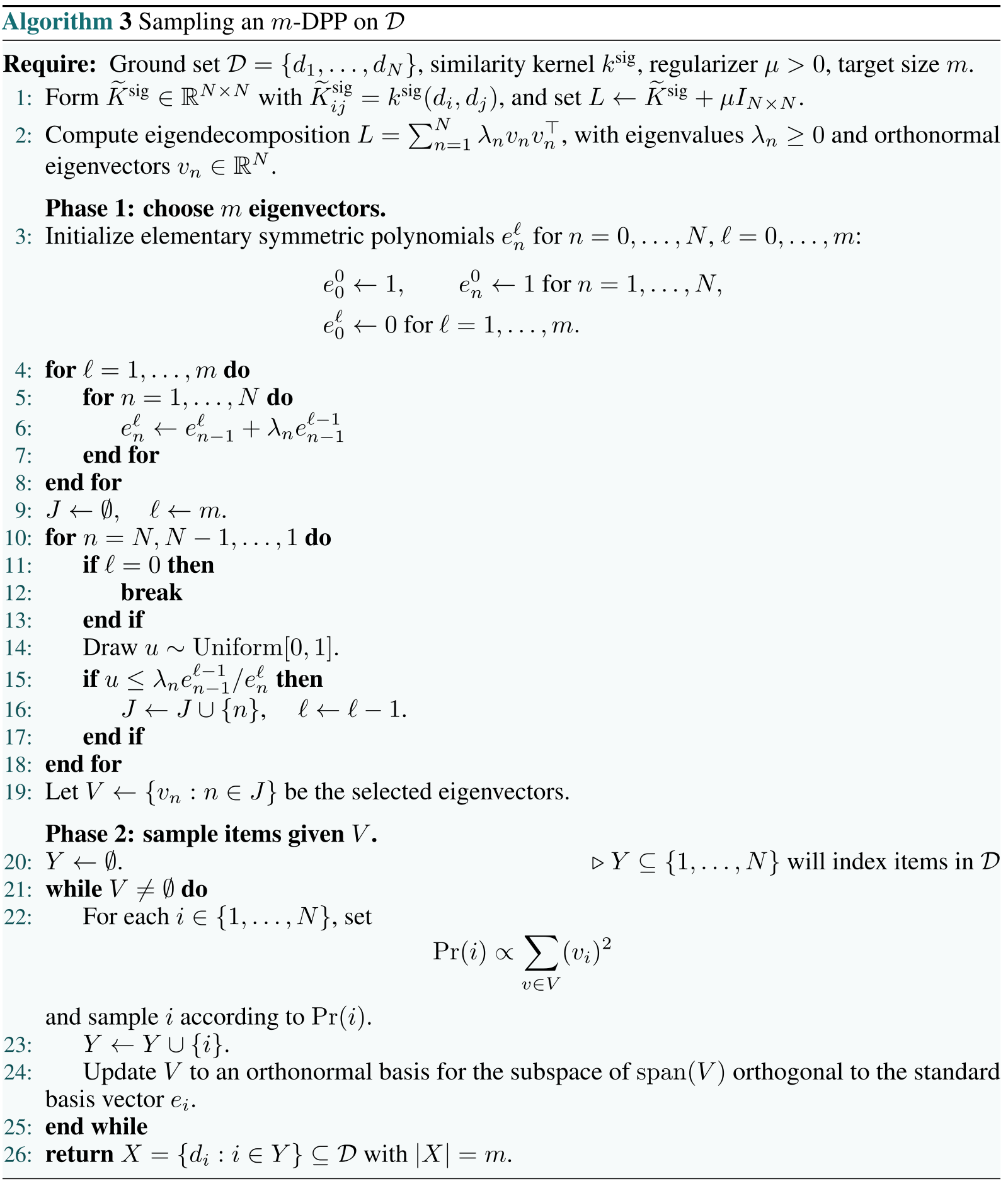
F.3 Determinantal sampling
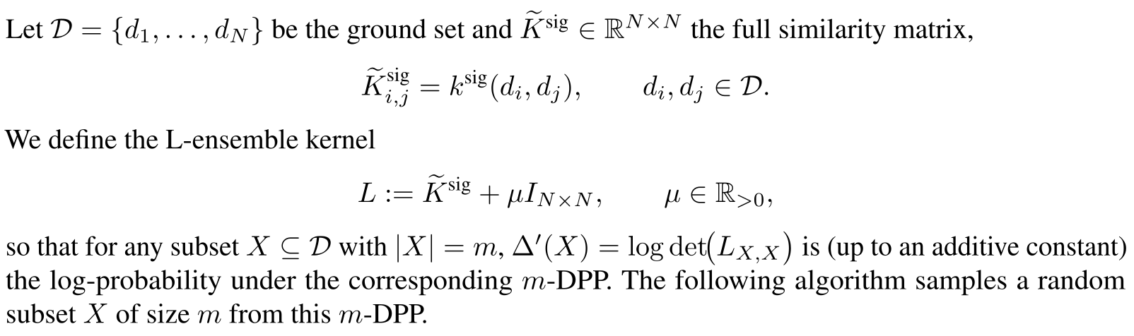
Algorithm 3 samples a size-m determinantal point process: choose eigenvectors using elementary symmetric polynomials, then sample items while updating an orthogonal basis. The complete 26-line algorithm is retained [78].
Sampling favors high-determinant subsets but is not maximum-a-posteriori optimization. With diagonal regularization, the determinant being sampled is that of the regularized kernel.
Equation
G.1 RoboMimic setup
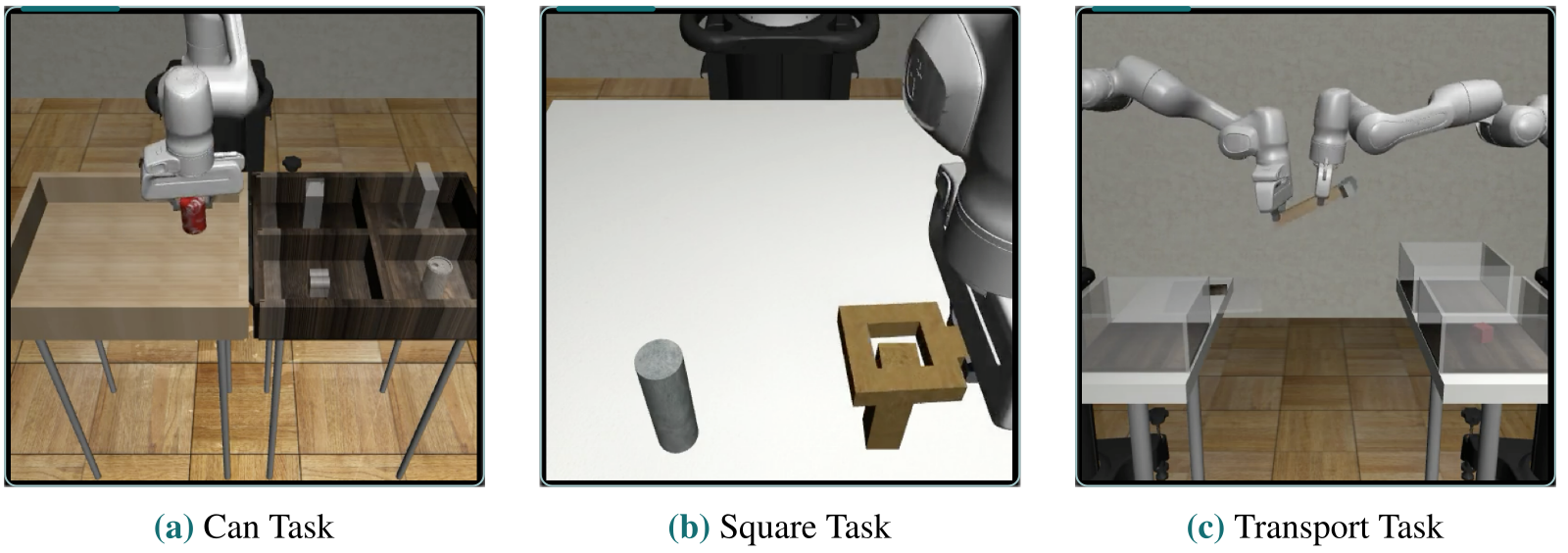
Can transfers a can between bins; Square places a nut over a rod; Transport requires two arms to transfer a hammer while clearing a target bin. Figure 8 retains all three scenes.
PH has 200 demonstrations from one experienced teleoperator. MH has 300 from six operators across three proficiency groups. The setup states train/validation splits of 180/20 and 270/30, whereas Table 6 labels MH full data as 280; that unresolved difference is preserved.
G.1.3 Policy settings
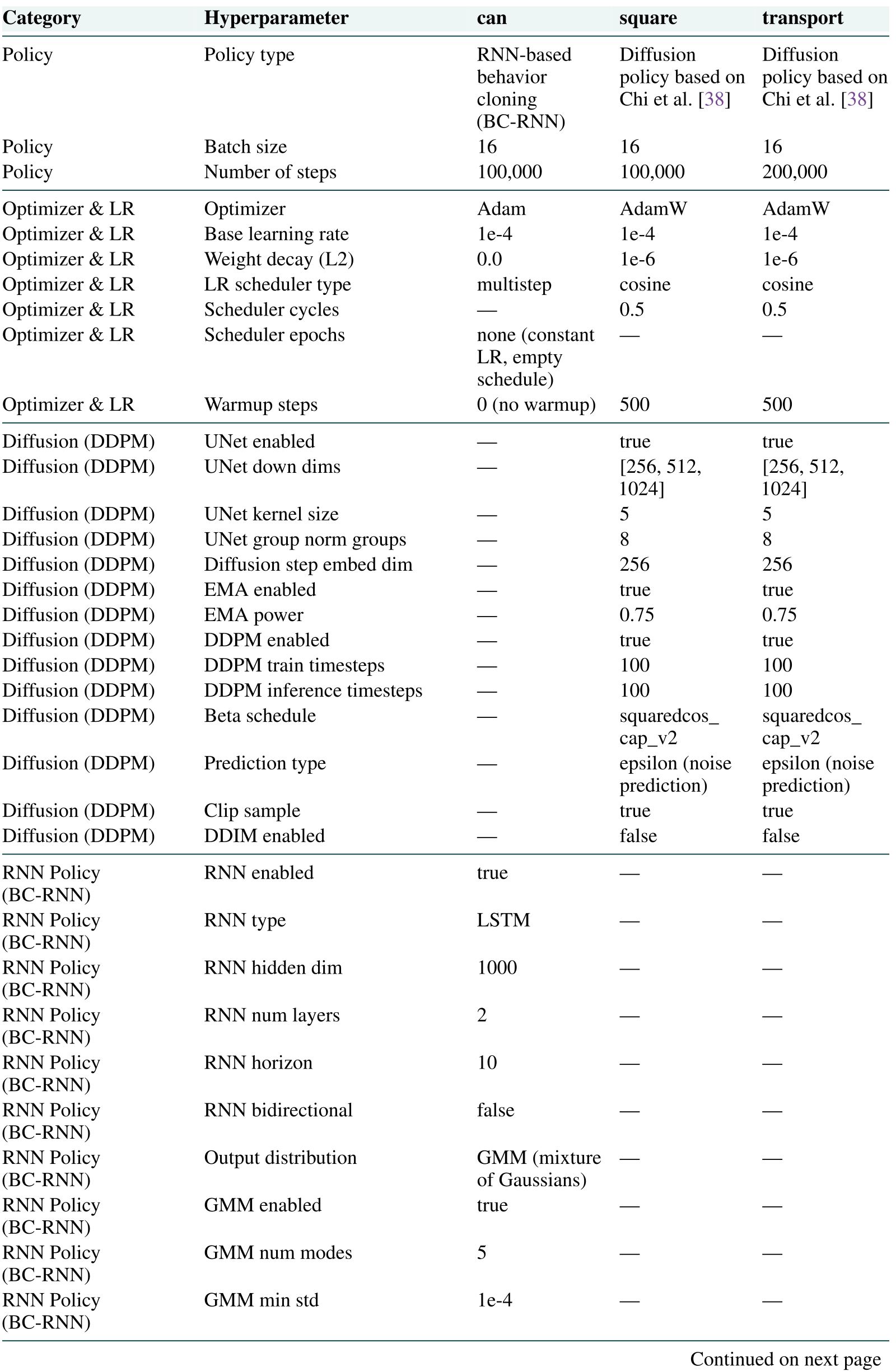
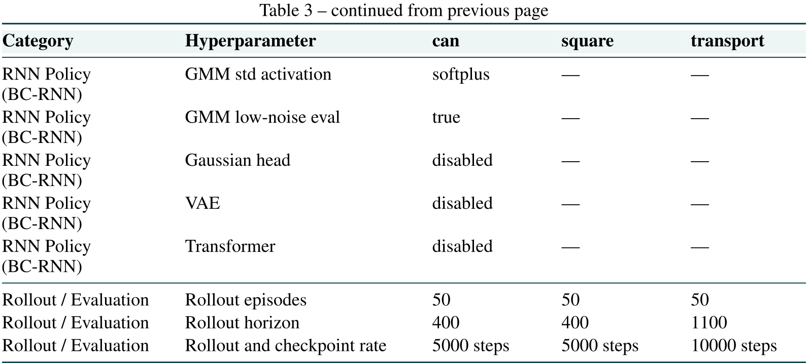
Table 3 is retained across both pages. Can uses a two-layer LSTM with 1,000 hidden units and a five-mode Gaussian mixture. Square and Transport use diffusion policies with 100 training and inference diffusion steps.
Batch size is 16. Training uses 100,000 steps for Can and Square and 200,000 for Transport; evaluation has 50 rollouts at each checkpoint. The main-text footnote’s claim of 100% Can full-data success differs from the Table 6 full-data values.
G.2 MetaWorld setup
Door Open, Stick Push, and Shelf Place each use 50 demonstrations, with randomized task and goal positions. Figure 9 preserves all scenes. The paper says the cited sources do not disclose how those demonstrations were collected.
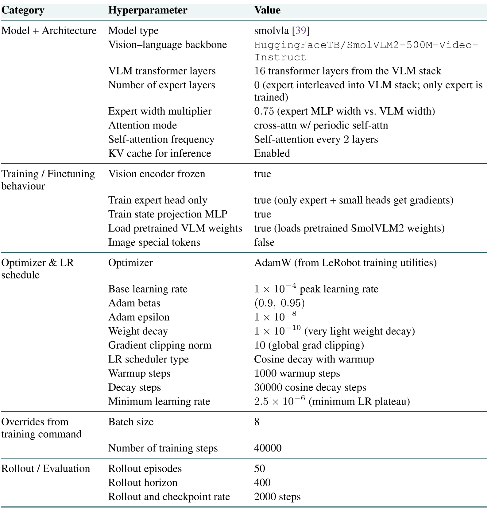
G.2.3 Policy settings
Table 4 retains the full SmolVLA configuration and exact backbone identifier. The vision encoder is frozen; the expert, small heads, and state projection are trained. Batch size is eight, training lasts 40,000 steps, and evaluation occurs every 2,000 steps with 50 rollouts.
G.3 Real-world setup
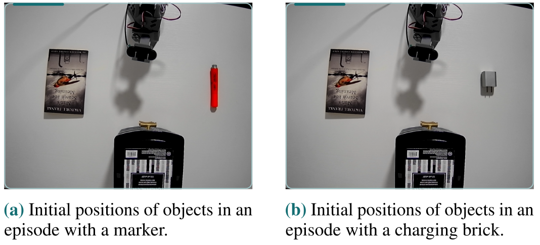
Drawer and marker tasks contain 50 demonstrations each; object organization and mug dragging contain 100, from one experienced teleoperator. Marker evaluation adds two unseen locations to the five collection locations. Objects are never presented in both organization branches simultaneously.
Policies receive wrist and overhead views, plus a side view for drawer and organization tasks. Cameras record 640×480 RGB at 30 frames per second. Figures 10 and 11 preserve all task views and conditional starting scenes.
G.3.3 Policy settings
The real-task setup follows Table 4 with batch size 64, 60,000 training steps, and evaluation every 20,000 steps. That implies three scheduled evaluations, conflicting with Figure 6’s “20 checkpoints” caption. The source does not resolve which evaluation protocol produced that figure.
H.1 Signature-level results
Figure 12 retains both Can variants, three-seed min/max bars, m=120, and p=0. It varies signature depth rather than dataset size. The differing curve shapes support task-dependent truncation, not a universal best depth.
H.2 Full results
Tables 5 and 6 retain every seed, summary value, budget, full-data reference, and continuation page. Their min/max columns describe seed ranges, not statistical confidence intervals.
Two Stick Push FAKTUAL rows in Table 5 are inconsistent with their printed seeds: at 25 demonstrations the seeds 0.44/0.26/0.22 imply mean ≈0.307 and minimum 0.22, not 0.29/0.18; at 35 demonstrations 0.46/0.26/0.20 imply mean ≈0.307 and minimum 0.20, not 0.30/0.18. Original values are preserved rather than silently corrected.
I. Proof
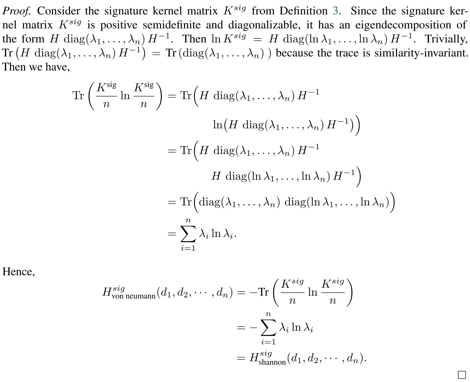
Lemma 1 and its complete proof show why normalized kernel-spectrum entropy equals matrix entropy. The trace is invariant under a change to the eigenvector basis.
The proof’s introductory sentence names eigenvalues of K, while subsequent equalities need eigenvalues of K/n. Read the λ values as the normalized spectrum, as specified in Definition 3; zero eigenvalues require the continuous 0 log 0 convention.