Literature
Display
← All papers

Cost-Driven Representation Learning for Linear Quadratic Gaussian Control: Part II

Yi Tian · Kaiqing Zhang · Russ Tedrake · Suvrit Sra

Preprint posted · arXiv (preprint) ↗

Control theory10 min text · CondensedOriginal paper ↗
Contents

At a glance

The paper studies learning a control-relevant state from a finite history of observations and actions by predicting cumulative quadratic costs. Two algorithms estimate latent dynamics either directly or through future-cost prediction plus coordinate alignment. The authors claim finite-sample guarantees for stable, partially observed linear–Gaussian systems. Several proof steps and a numerical lemma are incorrect as printed, so the rates below are reported claims rather than independently validated guarantees.

1 Introduction

Observation reconstruction can preserve irrelevant detail; inverse-action prediction targets controllability; cost prediction targets the control objective. This work develops the last approach for stationary, infinite-horizon LQG, extending the time-varying finite-horizon Part I. It connects a classical identification problem to the cost/value-prediction idea behind MuZero.

The key difficulty is statistical dependence within one exploration trajectory. Quadratic regression lifts history vectors into products of Gaussian variables; a new excitation argument and a proposed mixing-based concentration analysis support the claimed rates. The practical insight is that independently learned latent factors can use incompatible coordinates even when they predict identical costs.

This edition covers all 38 pages of v1, dated 8 March 2026. It preserves both complete algorithms, all 184 display containers, the exact assumption/definition/proposition/theorem/lemma statements and all 38 references. There are no empirical experiments or numbered graphical figures in this theoretical paper.

2 Problem setup

The hidden state obeys xₜ₊₁=A*xₜ+B*uₜ+wₜ; observations are yₜ=C*xₜ+vₜ. Process/measurement noises and the initial state are Gaussian. Minimize infinite-horizon time-averaged expected quadratic cost with positive semidefinite state cost Q* and positive definite action cost R*. Dynamics, observation model and noise covariances are unknown; R* is initially treated as known.

Assumption 1 requires open-loop stability, controllability through actions and process noise, observability through measurements and costs, full-rank observation noise, positive action penalties and bounded conditioning. These are substantial restrictions; the result does not cover arbitrary unstable, nonlinear or weakly identifiable systems. Stability/mixing constants still govern history length and sample requirements.

With known parameters, the separation principle combines a Kalman state estimate with the LQR gain obtained from algebraic Riccati equations. The exact optimum uses the recursive filter; the learned finite-history policy will incur truncation error.

Equations 2.1–2.3
xt+1=A∗​xt+B∗​ut+wt,yt=C∗​xt+vt,\displaystyle x_{t+1}=A^{\ast}x_{t}+B^{\ast}u_{t}+w_{t},\quad y_{t}=C^{\ast}x_{t}+v_{t}, (2.1)
c⁡(x,u)=‖x‖Q∗2+‖u‖R∗2,\displaystyle c(x,u)=\|x\|_{Q^{\ast}}^{2}+\|u\|_{R^{\ast}}^{2}, (2.2)
J⁡(π):=lim supT→∞1T​∑t=0T−1𝔼⁡[ct]\displaystyle J(\pi):=\limsup_{T\to\infty}\frac{1}{T}\sum\nolimits_{t=0}^{T-1}\mathbb{E}[c_{t}] (2.3)
Assumption 1.

System dynamics (2.1) and cost (2.2) satisfy:

  1. The system is stable, that is, ρ⁡(A∗)<1\rho(A^{\ast})<1.

  2. (A∗,B∗)(A^{\ast},B^{\ast}) is ν\nu-controllable for some ν>0\nu>0, that is, the controllability matrix

    Equation
    Φc​(A∗,B∗):=[B∗,A∗​B∗,…,(A∗)dx−1​B∗]\displaystyle\Phi_{c}(A^{\ast},B^{\ast}):=[B^{\ast},A^{\ast}B^{\ast},\ldots,(A^{\ast})^{d_{x}-1}B^{\ast}]

    has rank dxd_{x} and σmin​(Φc​(A∗,B∗))≥ν\sigma_{\min}(\Phi_{c}(A^{\ast},B^{\ast}))\geq\nu.

  3. (A∗,C∗)(A^{\ast},C^{\ast}) is ω\omega-observable for some ω>0\omega>0, that is, the observability matrix

    Equation
    Φo​(A∗,C∗):=[C∗;C∗​A∗;…;C∗​(A∗)dx−1]\displaystyle\Phi_{o}(A^{\ast},C^{\ast}):=[C^{\ast};C^{\ast}A^{\ast};\ldots;C^{\ast}(A^{\ast})^{d_{x}-1}]

    has rank dxd_{x} and σmin​(Φo​(A∗,C∗))≥ω\sigma_{\min}(\Phi_{o}(A^{\ast},C^{\ast}))\geq\omega.

  4. (A∗,Σw1/2)(A^{\ast},\Sigma_{w}^{1/2}) is κ\kappa-controllable for some κ>0\kappa>0.

  5. (A∗,(Q∗)1/2)(A^{\ast},(Q^{\ast})^{1/2}) is μ\mu-observable for some μ>0\mu>0.

  6. Σv≽σv2​I\Sigma_{v}\succcurlyeq\sigma_{v}^{2}I for some σv>0\sigma_{v}>0; this can always be achieved by inserting Gaussian noises with full-rank covariance matrices to the observations.

  7. R∗≽r2​IR^{\ast}\succcurlyeq r^{2}I for some r>0r>0.

  8. The operator norms of A∗A^{\ast}, B∗B^{\ast}, C∗C^{\ast}, Q∗Q^{\ast}, R∗R^{\ast}, Σw\Sigma_{w}, Σv\Sigma_{v}, Σ0\Sigma_{0} and α⁡(A∗),α⁡(A¯∗)\alpha(A^{\ast}),\alpha(\overline{A}^{\ast}) are 𝒪⁡(1)\mathcal{O}(1), the singular value lower bounds ν\nu, ω\omega, ν\nu, κ\kappa, σv\sigma_{v}, rr and spectral radii ρ⁡(A∗),ρ⁡(A¯∗)\rho(A^{\ast}),\rho(\overline{A}^{\ast}) are Ω⁡(1)\Omega(1), where A¯∗:=(I−L∗​C∗)​A∗\overline{A}^{\ast}:=(I-L^{\ast}C^{\ast})A^{\ast} with L∗L^{\ast} defined in (2.5).

Equations 2.4–2.8
zt+1∗=A∗​zt∗+B∗​ut+L∗​(yt+1−C∗​(A∗​zt∗+B∗​ut))\displaystyle z^{\ast}_{t+1}=A^{\ast}z^{\ast}_{t}+B^{\ast}u_{t}+L^{\ast}(y_{t+1}-C^{\ast}(A^{\ast}z^{\ast}_{t}+B^{\ast}u_{t})) (2.4)
L∗=\displaystyle L^{\ast}=\; S∗​(C∗)⊤​(C∗​S∗​(C∗)⊤+Σv)−1,\displaystyle S^{\ast}(C^{\ast})^{\top}(C^{\ast}S^{\ast}(C^{\ast})^{\top}+\Sigma_{v})^{-1}, (2.5)
K∗=\displaystyle K^{\ast}=\; −((B∗)⊤​P∗​B∗+R)−1​(B∗)⊤​P∗​A∗,\displaystyle-((B^{\ast})^{\top}P^{\ast}B^{\ast}+R)^{-1}(B^{\ast})^{\top}P^{\ast}A^{\ast}, (2.6)
Original PDF mathematical display S2.EGx8
Original selectable MathML
S∗=A∗​(S∗−S∗​(C∗)⊤​(CLOSECLOSEOPENOPENC∗​S∗​(C∗)⊤+Σv)−1​C∗​S∗)​(A∗)⊤+Σw,\displaystyle\begin{aligned} S^{\ast}=A^{\ast}\big(S^{\ast}-S^{\ast}(C^{\ast})^{\top}(&C^{\ast}S^{\ast}(C^{\ast})^{\top}+\Sigma_{v})^{-1}C^{\ast}S^{\ast}\big)(A^{\ast})^{\top}+\Sigma_{w},\end{aligned} (2.7)
P∗=(A∗)⊤​(P∗−P∗​B∗​(CLOSECLOSEOPENOPEN(B∗)⊤​P∗​B∗+R∗)−1​(B∗)⊤​P∗)​A∗+Q∗.\displaystyle\begin{aligned} P^{\ast}=(A^{\ast})^{\top}\big(P^{\ast}-P^{\ast}B^{\ast}(&(B^{\ast})^{\top}P^{\ast}B^{\ast}+R^{\ast})^{-1}(B^{\ast})^{\top}P^{\ast}\big)A^{\ast}+Q^{\ast}.\end{aligned} (2.8)

2.1 Latent model of infinite-horizon time-invariant LQG

Assume the Kalman error covariance is stationary at initialization. Proposition 1 expresses filtered states as a linear system driven by independent innovations; observed cost equals a quadratic function of the estimate plus a policy-independent constant and centered noise. The constant can be ignored when choosing actions, but the noise matters for learning.

Unroll the filter and retain H recent observations and actions. This defines z*ₜ=M*hₜ+δₜ, where δₜ decays with the stable filter dynamics. History dimension is dₕ=H(dᵧ+dᵤ). The policy combines a representation matrix M with latent feedback K. Initial H steps can use zero/Gaussian inputs because the open-loop system is assumed stable. Finite history approximates, rather than equals, the optimal recursive estimator.

Equation 2.9
zt+1∗=A∗​zt∗+B∗​ut+Lt+1∗​(yt+1−C∗​(A∗​zt∗+B∗​ut)),\displaystyle z^{\ast}_{t+1}=A^{\ast}z^{\ast}_{t}+B^{\ast}u_{t}+L^{\ast}_{t+1}(y_{t+1}-C^{\ast}(A^{\ast}z^{\ast}_{t}+B^{\ast}u_{t})), (2.9)
Proposition 1.

Let z0∗z^{\ast}_{0} be the initial state estimate and (zt∗)t≥1(z^{\ast}_{t})_{t\geq 1} be the state estimates given by the Kalman filter. Then, for t≥0t\geq 0,

Equation
zt+1∗=A∗​zt∗+B∗​ut+L∗​it+1,\displaystyle z^{\ast}_{t+1}=A^{\ast}z^{\ast}_{t}+B^{\ast}u_{t}+L^{\ast}i_{t+1},

where L∗​it+1L^{\ast}i_{t+1} is independent of zt∗z^{\ast}_{t} and utu_{t}, i.e., the state estimates follow the same linear dynamics with noises {L∗​it+1}t≥0\{L^{\ast}i_{t+1}\}_{t\geq 0}. The cost at step tt can be reformulated as a function of the state estimates by

Equation
ct=‖zt∗‖Q∗2+‖ut‖R∗2+b∗+γt+ηt,\displaystyle c_{t}=\|z^{\ast}_{t}\|_{Q^{\ast}}^{2}+\|u_{t}\|_{R^{\ast}}^{2}+b^{\ast}+\gamma_{t}+\eta_{t},

where b∗=𝔼⁡[‖xt−zt∗‖Q∗2]>0b^{\ast}=\mathbb{E}[\|x_{t}-z^{\ast}_{t}\|_{Q^{\ast}}^{2}]>0, and γt=‖xt−zt∗‖Q∗2−b∗\gamma_{t}=\|x_{t}-z^{\ast}_{t}\|_{Q^{\ast}}^{2}-b^{\ast}, ηt=2​⟨zt∗,xt−zt∗⟩Q∗\eta_{t}=2\bigl\langle z^{\ast}_{t},x_{t}-z^{\ast}_{t}\bigr\rangle_{Q^{\ast}} are both zero-mean subexponential random variables. Moreover, b∗=𝒪⁡(1)b^{\ast}=\mathcal{O}(1) and ‖γt‖ψ1=𝒪⁡(dx1/2)\|\gamma_{t}\|_{\psi_{1}}=\mathcal{O}(d_{x}^{1/2}); if control ut∼𝒩⁡(0,σu2​I)u_{t}\sim\mathcal{N}(0,\sigma_{u}^{2}I) for t≥0t\geq 0, then we have ‖ηt‖ψ1=𝒪⁡(dx1/2)\|\eta_{t}\|_{\psi_{1}}=\mathcal{O}(d_{x}^{1/2}).

Equations 2.10
zt∗\displaystyle z^{\ast}_{t} =A¯∗​(A¯∗​zt−2∗+B¯∗​ut−2+L∗​yt−1)+B¯∗​ut−1+L∗​yt\displaystyle=\overline{A}^{\ast}(\overline{A}^{\ast}z^{\ast}_{t-2}+\overline{B}^{\ast}u_{t-2}+L^{\ast}y_{t-1})+\overline{B}^{\ast}u_{t-1}+L^{\ast}y_{t}
=[(A¯∗)t−1L∗,…,L∗]y1:t+[(A¯∗)t−1B¯∗,…,B¯∗]u0:(t−1)+(A¯∗)tz0∗\displaystyle=[(\overline{A}^{\ast})^{t-1}L^{\ast},\ldots,L^{\ast}]y_{1:t}+[(\overline{A}^{\ast})^{t-1}\overline{B}^{\ast},\ldots,\overline{B}^{\ast}]u_{0:(t-1)}+(\overline{A}^{\ast})^{t}z^{\ast}_{0}
=:Mt∗[y1:t;u0:(t−1);z0∗],\displaystyle=:M^{\ast}_{t}[y_{1:t};u_{0:(t-1)};z^{\ast}_{0}],
zt∗\displaystyle z^{\ast}_{t} =[(A¯∗)H−1L∗,…,L∗]y(t−H+1):t+[(A¯∗)H−1B¯∗,…,B¯∗]u(t−H):(t−1)+δt\displaystyle=[(\overline{A}^{\ast})^{H-1}L^{\ast},\ldots,L^{\ast}]y_{(t-H+1):t}+[(\overline{A}^{\ast})^{H-1}\overline{B}^{\ast},\ldots,\overline{B}^{\ast}]u_{(t-H):(t-1)}+\delta_{t}
=:M∗[y(t−H+1):t;u(t−H):(t−1)]+δt,\displaystyle=:M^{\ast}[y_{(t-H+1):t};u_{(t-H):(t-1)}]+\delta_{t}, (2.10)

3 Method

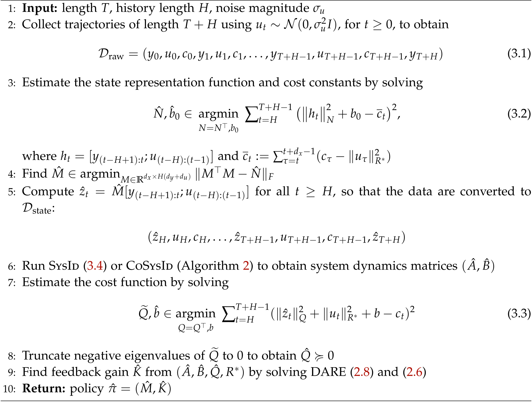
Collect one trajectory using independent zero-mean Gaussian exploration actions. Algorithm 1 regresses cumulative state costs on quadratic history features, factors the result into a latent representation, estimates dynamics and one-step cost, projects the cost matrix to be positive semidefinite, then solves the latent Riccati equation. Multiple independent trajectories can also supply the data.

The printed data range ends its costs at T+H−1, but its final dₓ-step target needs costs through T+H+dₓ−2; CoSysId’s shifted target needs one further step. Implementation therefore requires a longer trajectory or a shortened valid regression range. The original algorithms are retained without silently changing their indices.

Algorithm 1 Cost-driven state representation learning
Complete original PDF alg1
Original selectable source
1: Input: length TT, history length HH, noise magnitude σu\sigma_{u}
2: Collect trajectories of length T+HT+H using ut∼𝒩⁡(0,σu2​I)u_{t}\sim\mathcal{N}(0,\sigma_{u}^{2}I), for t≥0t\geq 0, to obtain
Equation 3.1
𝒟raw=\displaystyle\mathcal{D}_{\textnormal{raw}}= (y0,u0,c0,y1,u1,c1,…,yT+H−1,uT+H−1,cT+H−1,yT+H)\displaystyle(y_{0},u_{0},c_{0},y_{1},u_{1},c_{1},\ldots,y_{T+H-1},u_{T+H-1},c_{T+H-1},y_{T+H}) (3.1)
3: Estimate the state representation function and cost constants by solving
Equation 3.2
N^,b^0∈\displaystyle\hat{N},\hat{b}_{0}\in\; argminN=N⊤,b0∑t=HT+H−1(∥ht∥N2+b0−c¯t)2,\displaystyle\argmin_{N=N^{\top},b_{0}}~~\sum\nolimits_{t=H}^{T+H-1}\big(\big\|h_{t}\big\|_{N}^{2}+b_{0}-\overline{c}_{t}\big)^{2}, (3.2)
where ht=[y(t−H+1):t;u(t−H):(t−1)]h_{t}=[y_{(t-H+1):t};u_{(t-H):(t-1)}] and c¯t:=∑τ=tt+dx−1(cτ−‖uτ‖R∗2)\overline{c}_{t}:=\sum_{\tau=t}^{t+d_{x}-1}(c_{\tau}-\|u_{\tau}\|_{R^{\ast}}^{2})
4: Find M^∈argminM∈ℝdx×H⁡(dy+du)‖M⊤​M−N^‖F\hat{M}\in\argmin_{M\in\mathbb{R}^{d_{x}\times H(d_{y}+d_{u})}}\|M^{\top}M-\hat{N}\|_{F}
5: Compute z^t=M^[y(t−H+1):t;u(t−H):(t−1)]\hat{z}_{t}=\hat{M}[y_{(t-H+1):t};u_{(t-H):(t-1)}] for all t≥Ht\geq H, so that the data are converted to 𝒟state\mathcal{D}_{\textnormal{state}}:
Equation
(z^H,uH,cH,…,z^T+H−1,uT+H−1,cT+H−1,z^T+H)\displaystyle(\hat{z}_{H},u_{H},c_{H},\ldots,\hat{z}_{T+H-1},u_{T+H-1},c_{T+H-1},\hat{z}_{T+H})
6: Run SysId (3.4) or CoSysId (Algorithm 2) to obtain system dynamics matrices (A^,B^)(\hat{A},\hat{B})
7: Estimate the cost function by solving
Equation 3.3
Q~,b^∈argminQ=Q⊤,b∑t=HT+H−1(∥z^t∥Q2+∥ut∥R∗2+b−ct)2\displaystyle\widetilde{Q},\hat{b}\in\argmin_{Q=Q^{\top},b}~~\sum\nolimits_{t=H}^{T+H-1}(\|\hat{z}_{t}\|_{Q}^{2}+\|u_{t}\|_{R^{\ast}}^{2}+b-c_{t})^{2} (3.3)
8: Truncate negative eigenvalues of Q~\widetilde{Q} to 00 to obtain Q^≽0\hat{Q}\succcurlyeq 0
9: Find feedback gain K^\hat{K} from (A^,B^,Q^,R∗)(\hat{A},\hat{B},\hat{Q},R^{\ast}) by solving DARE (2.8) and (2.6)
10: Return: policy π^=(M^,K^)\hat{\pi}=(\hat{M},\hat{K})

3.1 Cost-driven representation function learning

The dₓ-step cost observability Gramian is positive definite under cost observability. In normalized coordinates it becomes identity, so regressing cumulative costs estimates N*=M*ᵀM*. Subtract known action penalties to reduce target variance; the paper proposes learning R* later if it is unknown.

Factor the estimated symmetric matrix using its largest dₓ nonnegative eigenvalues. The resulting representation is identifiable only up to an orthogonal transformation. Proposition 2 uses action controllability to lower-bound latent covariance and argues that sufficiently long history makes M* full row rank, with smallest singular value of order ν/√H. An eigenvalue threshold can then reveal latent rank once estimation error is sufficiently small.

The text says dₓ need not be known, but the printed cumulative-cost horizon and factorization already use dₓ. An upper bound or adaptive horizon procedure would be needed to operationalize that claim; it is not specified. The normalization also changes coordinates, so raw-state recovery is not the target.

Equations
Q¯∗:=∑t=0dx−1((A∗)t)⊤​Q∗​(A∗)t≽μ2​I.\displaystyle\overline{Q}^{\ast}:=\sum\nolimits_{t=0}^{d_{x}-1}((A^{\ast})^{t})^{\top}Q^{\ast}(A^{\ast})^{t}\succcurlyeq\mu^{2}I.
A∗⁣′=(Q¯∗)1/2A∗(Q¯∗)−1/2,B∗⁣′=(Q¯∗)1/2B∗,C∗⁣′=C∗(Q¯∗)−1/2,\displaystyle A^{\ast\prime}=(\overline{Q}^{\ast})^{1/2}A^{\ast}(\overline{Q}^{\ast})^{-1/2},\quad B^{\ast\prime}=(\overline{Q}^{\ast})^{1/2}B^{\ast},\quad C^{\ast\prime}=C^{\ast}(\overline{Q}^{\ast})^{-1/2},
wt′=(Q¯∗)1/2wt,Q∗⁣′=(Q¯∗)−1/2Q∗(Q¯∗)−1/2.\displaystyle w_{t}^{\prime}=(\overline{Q}^{\ast})^{1/2}w_{t},\quad Q^{\ast\prime}=(\overline{Q}^{\ast})^{-1/2}Q^{\ast}(\overline{Q}^{\ast})^{-1/2}.
Proposition 2.

Under i.i.d. actions ut∼𝒩⁡(0,σu2​I)u_{t}\sim\mathcal{N}(0,\sigma_{u}^{2}I) for t≥0t\geq 0, λmin​(Cov⁡(zt∗))=Ω⁡(ν2)\lambda_{\min}(\mathrm{Cov}(z_{t}^{\ast}))=\Omega(\nu^{2}) for t≥dxt\geq d_{x}, where ν\nu is defined in Assumption 1.2. Recall that for a square matrix AA, we define α⁡(A):=supk≥0‖Ak‖2​ρ​(A)−k\alpha(A):=\sup_{k\geq 0}\|A^{k}\|_{2}\rho(A)^{-k}. There exists a dimension-free constant a>0a>0, such that as long as H≥log⁡(a​α​(A¯∗))log⁡(ρ​(A¯∗)−1)H\geq\frac{\log(a\alpha(\overline{A}^{\ast}))}{\log(\rho(\overline{A}^{\ast})^{-1})}, M∗M^{\ast} has rank dxd_{x} and σmin(M∗)=Ω(νH−1/2)\sigma_{\min}(M^{\ast})=\Omega(\nu H^{-1/2}).

Equations
zt∗=\displaystyle z^{\ast}_{t}=\; A∗​zt−1∗+B∗​ut−1+L∗​it\displaystyle A^{\ast}z^{\ast}_{t-1}+B^{\ast}u_{t-1}+L^{\ast}i_{t}
=\displaystyle=\; A∗​(A∗​zt−2∗+B∗​ut−2+L∗​it−1)+L∗​it\displaystyle A^{\ast}(A^{\ast}z^{\ast}_{t-2}+B^{\ast}u_{t-2}+L^{\ast}i_{t-1})+L^{\ast}i_{t}
=\displaystyle=\; [B∗,…,(A∗)dx−1​B∗]​[ut−1;…;ut−dx]+(A∗)dx​zt−dx∗+[L∗,…,(A∗)dx−1​L∗]​[it;…;it−dx+1],\displaystyle[B^{\ast},\ldots,(A^{\ast})^{d_{x}-1}B^{\ast}][u_{t-1};\ldots;u_{t-d_{x}}]+(A^{\ast})^{d_{x}}z^{\ast}_{t-d_{x}}+[L^{\ast},\ldots,(A^{\ast})^{d_{x}-1}L^{\ast}][i_{t};\ldots;i_{t-d_{x}+1}],
Cov⁡(zt∗)=𝔼⁡[zt∗​(zt∗)⊤]≽\displaystyle\mathrm{Cov}(z^{\ast}_{t})=\mathbb{E}[z^{\ast}_{t}(z^{\ast}_{t})^{\top}]\succcurlyeq\; Φc​(A∗,B∗)​𝔼​[[ut−1;…;ut−ℓ]​[ut−1;…;ut−ℓ]⊤]​Φc⊤​(A∗,B∗)\displaystyle\Phi_{c}(A^{\ast},B^{\ast})\mathbb{E}[[u_{t-1};\ldots;u_{t-\ell}][u_{t-1};\ldots;u_{t-\ell}]^{\top}]\Phi_{c}^{\top}(A^{\ast},B^{\ast})
=\displaystyle=\; σu2​Φc​(A∗,B∗)​Φc⊤​(A∗,B∗).\displaystyle\sigma_{u}^{2}\Phi_{c}(A^{\ast},B^{\ast})\Phi_{c}^{\top}(A^{\ast},B^{\ast}).
Cov⁡(M∗​ht)=Cov⁡(zt∗−δt)=Cov⁡(zt∗)+Cov⁡(δt)−Cov⁡(zt∗,δt)−Cov⁡(δt,zt∗).\displaystyle\mathrm{Cov}(M^{\ast}h_{t})=\mathrm{Cov}(z^{\ast}_{t}-\delta_{t})=\mathrm{Cov}(z^{\ast}_{t})+\mathrm{Cov}(\delta_{t})-\mathrm{Cov}(z^{\ast}_{t},\delta_{t})-\mathrm{Cov}(\delta_{t},z^{\ast}_{t}).
‖Cov⁡(zt∗,δt)‖2=‖Cov⁡(δt,zt∗)‖2=\displaystyle\|\mathrm{Cov}(z^{\ast}_{t},\delta_{t})\|_{2}=\|\mathrm{Cov}(\delta_{t},z^{\ast}_{t})\|_{2}=\; ‖𝔼⁡[zt∗​δt⊤]‖2\displaystyle\|\mathbb{E}[z^{\ast}_{t}\delta_{t}^{\top}]\|_{2}
≤(i)\displaystyle\overset{(i)}{\leq}\; ‖𝔼⁡[zt∗​(zt∗)⊤]‖21/2⋅‖𝔼⁡[δt​δt⊤]‖21/2\displaystyle\|\mathbb{E}[z^{\ast}_{t}(z^{\ast}_{t})^{\top}]\|_{2}^{1/2}\cdot\|\mathbb{E}[\delta_{t}\delta_{t}^{\top}]\|_{2}^{1/2}
=\displaystyle=\; ‖Cov⁡(zt∗)‖21/2⋅‖Cov⁡(δt)‖21/2,\displaystyle\|\mathrm{Cov}(z^{\ast}_{t})\|_{2}^{1/2}\cdot\|\mathrm{Cov}(\delta_{t})\|_{2}^{1/2},
λmin​(Cov⁡(M∗​ht))≥\displaystyle\lambda_{\min}(\mathrm{Cov}(M^{\ast}h_{t}))\geq\; λmin​(Cov⁡(zt∗))−2​‖Cov⁡(zt∗)‖21/2⋅‖Cov⁡(δt)‖21/2.\displaystyle\lambda_{\min}(\mathrm{Cov}(z^{\ast}_{t}))-2\|\mathrm{Cov}(z^{\ast}_{t})\|_{2}^{1/2}\cdot\|\mathrm{Cov}(\delta_{t})\|_{2}^{1/2}.
λmin​(Cov⁡(M∗​ht))≥σu2​ν2/2.\displaystyle\lambda_{\min}(\mathrm{Cov}(M^{\ast}h_{t}))\geq\sigma_{u}^{2}\nu^{2}/2.
𝔼⁡[M∗​ht​ht⊤​(M∗)⊤]≼‖𝔼⁡[ht​ht⊤]‖2​M∗​(M∗)⊤.\displaystyle\mathbb{E}[M^{\ast}h_{t}h_{t}^{\top}(M^{\ast})^{\top}]\preccurlyeq\|\mathbb{E}[h_{t}h_{t}^{\top}]\|_{2}M^{\ast}(M^{\ast})^{\top}.
0<σu2​ν2/2≤λmin​(Cov⁡(M∗​ht))=𝒪⁡(H)​σdx2​(M∗).\displaystyle 0<\sigma_{u}^{2}\nu^{2}/2\leq\lambda_{\min}(\mathrm{Cov}(M^{\ast}h_{t}))=\mathcal{O}(H)\sigma_{d_{x}}^{2}(M^{\ast}).

3.2 Explicit learning of system dynamics

CoReL-E fits A and B by least squares from estimated latent states and actions to the next estimated state. This follows the explicit transition-prediction route. Both input and output estimates contain learned-representation and truncation errors; Lemma 5 is intended to propagate those errors through the regression. No observation-reconstruction matrix C* needs to be learned.

Equation 3.4
(A^,B^)∈argminA,B∑t=HT+H−1∥Az^t+But−z^t+1∥2.\displaystyle(\hat{A},\hat{B})\in\argmin_{A,B}~~\sum\nolimits_{t=H}^{T+H-1}\|A\hat{z}_{t}+Bu_{t}-\hat{z}_{t+1}\|^{2}. (3.4)

3.3 Implicit learning of system dynamics (MuZero-style)

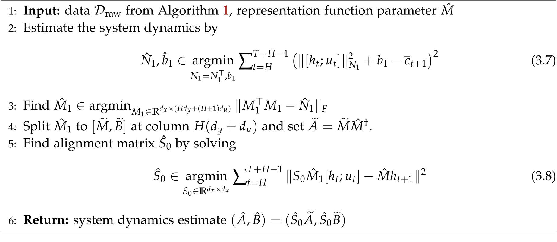
CoReL-I instead predicts current and one-step-ahead cumulative costs. Lifting MᵀM and [AM,B]ᵀ[AM,B] turns each cost fit into quadratic-feature linear regression. Separate intercepts decouple the two regressions. After factorization, estimate an alignment matrix between the current-state and predicted-next-state coordinates, then use aligned dynamics in the controller.

This alignment is necessary because cost norms are unchanged by orthogonal rotations, and the two factorizations need not choose the same rotation. Longer future-cost prediction is a suggested alternative, but the analyzed algorithm explicitly performs alignment rather than proving that arbitrary multi-step MuZero training resolves it.

The discussion rejecting a lower-dimensional regression contains a rank error: controllability of (A*,B*) implies [A*,B*] has full row rank. If M* also has full row rank, it has a right inverse and [A*M*,B*] has the same rank as [A*,B*]. The claimed rank distinction cannot justify choosing one regressor over the other under these assumptions.

Equations 3.5–3.6
∑t=HT+H−ℓ−1∑i=0ℓ(‖zt,i‖Q2+‖ut+i‖R∗2+b−ct+i)2.\displaystyle\sum\nolimits_{t=H}^{T+H-\ell-1}\sum\nolimits_{i=0}^{\ell}(\|z_{t,i}\|_{Q}^{2}+\|u_{t+i}\|_{R^{\ast}}^{2}+b-c_{t+i})^{2}.
minM,A,B,b\displaystyle\min_{M,A,B,b} ∑t=HT+H−1((‖M​ht‖2+b−c¯t)2+(‖A​M​ht+B​ut‖2+b−c¯t+1)2).\displaystyle\sum\nolimits_{t=H}^{T+H-1}\big((\|Mh_{t}\|^{2}+b-\overline{c}_{t})^{2}+(\|AMh_{t}+Bu_{t}\|^{2}+b-\overline{c}_{t+1})^{2}\big). (3.5)
minN,N1,b\displaystyle\min_{N,N_{1},b} ∑t=HT+H−1((‖ht‖N2+b−c¯t)2+(‖[ht;ut]‖N12+b−c¯t+1)2).\displaystyle\sum\nolimits_{t=H}^{T+H-1}\big((\|h_{t}\|_{N}^{2}+b-\overline{c}_{t})^{2}+(\|[h_{t};u_{t}]\|_{N_{1}}^{2}+b-\overline{c}_{t+1})^{2}\big). (3.6)
Algorithm 2 CoSysId: Cost-driven system identification
Complete original PDF alg2
Original selectable source
1: Input: data 𝒟raw\mathcal{D}_{\textnormal{raw}} from Algorithm 1, representation function parameter M^\hat{M}
2: Estimate the system dynamics by
Equation 3.7
N^1,b^1∈argminN1=N1⊤,b1∑t=HT+H−1(∥[ht;ut]∥N12+b1−c¯t+1)2\displaystyle\hat{N}_{1},\hat{b}_{1}\in\argmin_{N_{1}=N_{1}^{\top},b_{1}}\sum\nolimits_{t=H}^{T+H-1}\big(\|[h_{t};u_{t}]\|_{N_{1}}^{2}+b_{1}-\overline{c}_{t+1}\big)^{2} (3.7)
3: Find M^1∈argminM1∈ℝdx×(H​dy+(H+1)​du)‖M1⊤​M1−N^1‖F\hat{M}_{1}\in\argmin_{M_{1}\in\mathbb{R}^{d_{x}\times(Hd_{y}+(H+1)d_{u})}}\|M_{1}^{\top}M_{1}-\hat{N}_{1}\|_{F}
4: Split M^1\hat{M}_{1} to [M~,B~][\widetilde{M},\widetilde{B}] at column H⁡(dy+du)H(d_{y}+d_{u}) and set A~=M~​M^†\widetilde{A}=\widetilde{M}\hat{M}^{\dagger}.
5: Find alignment matrix S^0\hat{S}_{0} by solving
Equation 3.8
S^0∈argminS0∈ℝdx×dx∑t=HT+H−1∥S0M^1[ht;ut]−M^ht+1∥2\displaystyle\hat{S}_{0}\in\argmin_{S_{0}\in\mathbb{R}^{d_{x}\times d_{x}}}\sum\nolimits_{t=H}^{T+H-1}\|S_{0}\hat{M}_{1}[h_{t};u_{t}]-\hat{M}h_{t+1}\|^{2} (3.8)
6: Return: system dynamics estimate (A^,B^)=(S^0​A~,S^0​B~)(\hat{A},\hat{B})=(\hat{S}_{0}\widetilde{A},\hat{S}_{0}\widetilde{B})
Equation
N^2,b^2∈\displaystyle\hat{N}_{2},\hat{b}_{2}\in\; argminN2=N2⊤,b2∑t=HT+H−1(∥[z^t;ut]∥N22+b2−c¯t+1)2,\displaystyle\argmin_{N_{2}=N_{2}^{\top},b_{2}}~~\sum\nolimits_{t=H}^{T+H-1}\big(\|[\hat{z}_{t};u_{t}]\|_{N_{2}}^{2}+b_{2}-\overline{c}_{t+1}\big)^{2},

4 Theoretical guarantees and proofs

Theorem 1 claims an O(poly(H,dₓ,dᵧ,dᵤ,log(T/p))/T) average-cost gap with probability at least 1−p, after a polynomial sample threshold and H growing roughly as log(T/p)/log(1/ρ). The intended estimation errors scale as T⁻¹ᐟ² up to conditioning, dimension and logarithmic factors; the cost gap is quadratic in small controller error.

Compared with observation-based system identification, the authors acknowledge worse dimension dependence and a longer burn-in because scalar quadratic costs require a much larger feature space. The result is not a dimension-free practical sample budget. The proof issues documented below prevent treating the printed statement as fully established by this version.

Theorem 1.

Given an unknown LQG control problem defined by (2.1) and (2.2), under Assumption 1, for a given p∈(0,1)p\in(0,1), if we run CoReL-E (Algorithm 1 with (3.4)) or CoReL-I (Algorithm 1 with Algorithm 2) for T≥poly⁡(dx,dy,du,log⁡(T/p))T\geq\mathrm{poly}(d_{x},d_{y},d_{u},\log(T/p)), H=Ω⁡(log⁡(α​H​(dy+du)​T/p)log⁡(1/ρ))H=\Omega(\frac{\log(\alpha H(d_{y}+d_{u})T/p)}{\log(1/\rho)}), and σu=Θ⁡(1)\sigma_{u}=\Theta(1), then with probability at least 1−p1-p, the learned representation function M^\hat{M} is poly⁡(H,dx,du,dy,log⁡(T/p))\mathrm{poly}(H,d_{x},d_{u},d_{y},\log(T/p))-optimal, and the overall output policy π^=(M^,K^)\hat{\pi}=(\hat{M},\hat{K}) satisfies

Equation
J⁡(π^)−J⁡(π∗)=𝒪⁡(poly⁡(H,dx,du,dy,log⁡(T/p))​T−1).\displaystyle J(\hat{\pi})-J(\pi^{\ast})=\mathcal{O}(\mathrm{poly}(H,d_{x},d_{u},d_{y},\log(T/p))T^{-1}).

4.1 Proposition on multi-step cumulative costs

Proposition 3 aims to decompose dₓ-step cumulative state cost into squared latent norm, a constant, exponentially small history-truncation error and centered subexponential noise. It then seeks a √T-type bound for the sum of quadratic features times noise despite temporal dependence.

The proposed argument splits distant time indices into groups, conditionally centers each feature/noise product, and bounds the remaining conditional mean through mixing. However, the first cost expansion drops cross terms pointwise because the summands are independent. Independence removes their expectation, not their realized values; these terms must be included and controlled in the noise decomposition.

Conditional centering also creates martingale differences, not automatically independent variables as the proof states. Its cited concentration step needs a matching dependence argument. A later error recursion prints +vₜ₊₁ where direct algebra gives −L*vₜ₊₁. All source displays are retained; these observations identify gaps in the printed derivation rather than supplying a repaired proof.

Proposition 3.

Given an LQG control problem satisfying Assumption 1, let M∗M^{\ast} parameterize the optimal state representation function under the normalized parameterization. Recall that α:=max⁡(α⁡(A∗),α⁡(A¯∗))\alpha:=\max(\alpha(A^{\ast}),\alpha(\overline{A}^{\ast})) and ρ:=max⁡(ρ⁡(A∗),ρ⁡(A¯∗))\rho:=\max(\rho(A^{\ast}),\rho(\overline{A}^{\ast})). If we apply ut∼𝒩⁡(0,σu2​I)u_{t}\sim\mathcal{N}(0,\sigma_{u}^{2}I), then for any t≥Ht\geq H,

Equation
c¯t:=∑τ=tt+dx−1(cτ−‖uτ‖R∗2)=‖M∗​ht‖2+δ¯t+b¯∗+e¯t,\displaystyle\overline{c}_{t}:=\sum\nolimits_{\tau=t}^{t+d_{x}-1}(c_{\tau}-\|u_{\tau}\|_{R^{\ast}}^{2})=\|M^{\ast}h_{t}\|^{2}+\overline{\delta}_{t}+\overline{b}^{\ast}+\overline{e}_{t},

where δ¯t=𝒪⁡(α2​ρH​log⁡(T/p))\overline{\delta}_{t}=\mathcal{O}(\alpha^{2}\rho^{H}\log(T/p)) is a small error term, b¯∗=𝒪⁡(dx)\overline{b}^{\ast}=\mathcal{O}(d_{x}) is a positive constant, and e¯t\overline{e}_{t} is a zero-mean subexponential random variable with ‖e¯t‖ψ1=𝒪⁡(dx3/2)\|\overline{e}_{t}\|_{\psi_{1}}=\mathcal{O}(d_{x}^{3/2}). Moreover, let f¯t=[svec⁡(ht​ht⊤);1]\overline{f}_{t}=[\mathrm{svec}(h_{t}h_{t}^{\top});1]. There exists a dimension-free constant a>0a>0 such that for a given p∈(0,1)p\in(0,1), as long as H≥max⁡(dx−1,a​log⁡(α​T​log⁡(T/p))log⁡(1/ρ))H\geq\max(d_{x}-1,\frac{a\log(\alpha T\log(T/p))}{\log(1/\rho)}), (e¯t)t≥H(\overline{e}_{t})_{t\geq H} satisfy

Equation
‖∑t=HT+H−1f¯t​e¯t‖=𝒪⁡(dx3/2​dh​H1/2​T1/2​log1/2⁡(H/p)).\displaystyle\Big\|\sum\nolimits_{t=H}^{T+H-1}\overline{f}_{t}\overline{e}_{t}\Big\|=\mathcal{O}(d_{x}^{3/2}d_{h}H^{1/2}T^{1/2}\log^{1/2}(H/p)).
Equations 4.1–4.5
ct+ℓ−‖ut+ℓ‖R∗2=‖xt+ℓ‖Q∗2\displaystyle c_{t+\ell}-\|u_{t+\ell}\|_{R^{\ast}}^{2}=\|x_{t+\ell}\|_{Q^{\ast}}^{2}
=\displaystyle=\; ‖(A∗)ℓ​xt+Φc,ℓ​[ut+ℓ−1;…;ut]+∑i=1ℓ(A∗)i−1​wt+ℓ−i‖Q∗2\displaystyle\Big\|(A^{\ast})^{\ell}x_{t}+\Phi_{c,\ell}[u_{t+\ell-1};\ldots;u_{t}]+\sum\nolimits_{i=1}^{\ell}(A^{\ast})^{i-1}w_{t+\ell-i}\Big\|_{Q^{\ast}}^{2}
=(i)\displaystyle\overset{(i)}{=}\; ∥(A∗)ℓxt∥Q∗2+∥Φc,ℓu(t+ℓ−1):t∥Q∗2+∥∑i=1ℓ(A∗)i−1wt+ℓ−i∥Q∗2,\displaystyle\|(A^{\ast})^{\ell}x_{t}\|_{Q^{\ast}}^{2}+\|\Phi_{c,\ell}u_{(t+\ell-1):t}\|_{Q^{\ast}}^{2}+\Big\|\sum\nolimits_{i=1}^{\ell}(A^{\ast})^{i-1}w_{t+\ell-i}\Big\|_{Q^{\ast}}^{2},
ct+ℓ−‖ut+ℓ‖R∗2=\displaystyle c_{t+\ell}-\|u_{t+\ell}\|_{R^{\ast}}^{2}=\; ‖(A∗)ℓ​zt∗‖Q∗2+‖(A∗)ℓ​(xt−zt∗)‖Q∗2+2​⟨(A∗)ℓ​zt∗,(A∗)ℓ​(xt−zt∗)⟩Q∗\displaystyle\|(A^{\ast})^{\ell}z^{\ast}_{t}\|_{Q^{\ast}}^{2}+\|(A^{\ast})^{\ell}(x_{t}-z^{\ast}_{t})\|_{Q^{\ast}}^{2}+2\bigl\langle(A^{\ast})^{\ell}z^{\ast}_{t},(A^{\ast})^{\ell}(x_{t}-z^{\ast}_{t})\bigr\rangle_{Q^{\ast}}
+∥Φc,ℓu(t+ℓ−1):t∥Q∗2+∥∑i=1ℓ(A∗)i−1wt+ℓ−i∥Q∗2\displaystyle\quad+\|\Phi_{c,\ell}u_{(t+\ell-1):t}\|_{Q^{\ast}}^{2}+\Big\|\sum\nolimits_{i=1}^{\ell}(A^{\ast})^{i-1}w_{t+\ell-i}\Big\|_{Q^{\ast}}^{2}
=\displaystyle=\; ‖(A∗)ℓ​(M∗​ht+δt)‖Q∗2+‖(A∗)ℓ​(xt−zt∗)‖Q∗2+2​⟨(A∗)ℓ​zt∗,(A∗)ℓ​(xt−zt∗)⟩Q∗\displaystyle\|(A^{\ast})^{\ell}(M^{\ast}h_{t}+\delta_{t})\|_{Q^{\ast}}^{2}+\|(A^{\ast})^{\ell}(x_{t}-z^{\ast}_{t})\|_{Q^{\ast}}^{2}+2\bigl\langle(A^{\ast})^{\ell}z^{\ast}_{t},(A^{\ast})^{\ell}(x_{t}-z^{\ast}_{t})\bigr\rangle_{Q^{\ast}}
+∥Φc,ℓu(t+ℓ−1):t∥Q∗2+∥∑i=1ℓ(A∗)i−1wt+ℓ−i∥Q∗2\displaystyle\quad+\|\Phi_{c,\ell}u_{(t+\ell-1):t}\|_{Q^{\ast}}^{2}+\Big\|\sum\nolimits_{i=1}^{\ell}(A^{\ast})^{i-1}w_{t+\ell-i}\Big\|_{Q^{\ast}}^{2}
=\displaystyle=\; ‖(A∗)ℓ​M∗​ht‖Q∗2+δt,ℓ+bℓ∗+et,ℓ,\displaystyle\|(A^{\ast})^{\ell}M^{\ast}h_{t}\|_{Q^{\ast}}^{2}+\delta_{t,\ell}+b^{\ast}_{\ell}+e_{t,\ell},
bℓ∗:=\displaystyle b^{\ast}_{\ell}:=\; 𝔼[∥(A∗)ℓ(xt−zt∗)∥Q∗2+∥Φc,ℓu(t+ℓ−1):t∥Q∗2+∥∑i=1ℓ(A∗)i−1wt+ℓ−i∥Q∗2],\displaystyle\mathbb{E}\Big[\|(A^{\ast})^{\ell}(x_{t}-z^{\ast}_{t})\|_{Q^{\ast}}^{2}+\|\Phi_{c,\ell}u_{(t+\ell-1):t}\|_{Q^{\ast}}^{2}+\Big\|\sum\nolimits_{i=1}^{\ell}(A^{\ast})^{i-1}w_{t+\ell-i}\Big\|_{Q^{\ast}}^{2}\Big],
et,ℓ:=\displaystyle e_{t,\ell}:=\; ‖(A∗)ℓ​(xt−zt∗)‖Q∗2+2​⟨(A∗)ℓ​zt∗,(A∗)ℓ​(xt−zt∗)⟩Q∗\displaystyle\|(A^{\ast})^{\ell}(x_{t}-z^{\ast}_{t})\|_{Q^{\ast}}^{2}+2\bigl\langle(A^{\ast})^{\ell}z^{\ast}_{t},(A^{\ast})^{\ell}(x_{t}-z^{\ast}_{t})\bigr\rangle_{Q^{\ast}}
+∥Φc,ℓu(t+ℓ−1):t∥Q∗2+∥∑i=1ℓ(A∗)i−1wt+ℓ−i∥Q∗2−bℓ∗.\displaystyle\quad+\|\Phi_{c,\ell}u_{(t+\ell-1):t}\|_{Q^{\ast}}^{2}+\Big\|\sum\nolimits_{i=1}^{\ell}(A^{\ast})^{i-1}w_{t+\ell-i}\Big\|_{Q^{\ast}}^{2}-b^{\ast}_{\ell}.
ℱt:=σ⁡(x0,y0,u0,x1,y1,…,ut−1,xt,yt).\displaystyle\mathcal{F}_{t}:=\sigma(x_{0},y_{0},u_{0},x_{1},y_{1},\ldots,u_{t-1},x_{t},y_{t}).
c¯t=∑τ=tt+dx−1(cτ−‖uτ‖R∗2)=‖M∗​ht‖2+δ¯t+b¯∗+e¯t,\displaystyle\overline{c}_{t}=\sum\nolimits_{\tau=t}^{t+d_{x}-1}(c_{\tau}-\|u_{\tau}\|_{R^{\ast}}^{2})=\|M^{\ast}h_{t}\|^{2}+\overline{\delta}_{t}+\overline{b}^{\ast}+\overline{e}_{t},
∑ℓ=0dx−1⟨(A∗)ℓ​M∗​ht,(A∗)ℓ​δt⟩Q∗=∑ℓ=0dx−1(Mt∗​ht)⊤​((A∗)ℓ)⊤​Q∗​(A∗)ℓ​δt=(Mt∗​ht)⊤​δt=⟨M∗​ht,δt⟩\displaystyle\sum\nolimits_{\ell=0}^{d_{x}-1}\bigl\langle(A^{\ast})^{\ell}M^{\ast}h_{t},(A^{\ast})^{\ell}\delta_{t}\bigr\rangle_{Q^{\ast}}=\sum\nolimits_{\ell=0}^{d_{x}-1}(M^{\ast}_{t}h_{t})^{\top}((A^{\ast})^{\ell})^{\top}Q^{\ast}(A^{\ast})^{\ell}\delta_{t}=(M^{\ast}_{t}h_{t})^{\top}\delta_{t}=\bigl\langle M^{\ast}h_{t},\delta_{t}\bigr\rangle
δ¯t:=∑ℓ=0dx−1δt,ℓ=‖δt‖2+2​⟨M∗​ht,δt⟩,\displaystyle\overline{\delta}_{t}:=\sum\nolimits_{\ell=0}^{d_{x}-1}\delta_{t,\ell}=\|\delta_{t}\|^{2}+2\bigl\langle M^{\ast}h_{t},\delta_{t}\bigr\rangle,
b¯∗:=∑ℓ=0dx−1bℓ∗=𝔼[∥xt−zt∗∥2+∑ℓ=0dx−1(∥Φc,ℓu(t+ℓ−1):t∥Q∗2+∥∑i=1ℓ(A∗)i−1wt+ℓ−i∥Q∗2)],\displaystyle\overline{b}^{\ast}:=\sum\nolimits_{\ell=0}^{d_{x}-1}b^{\ast}_{\ell}=\mathbb{E}\Big[\|x_{t}-z^{\ast}_{t}\|^{2}+\sum\nolimits_{\ell=0}^{d_{x}-1}\Big(\|\Phi_{c,\ell}u_{(t+\ell-1):t}\|_{Q^{\ast}}^{2}+\Big\|\sum\nolimits_{i=1}^{\ell}(A^{\ast})^{i-1}w_{t+\ell-i}\Big\|_{Q^{\ast}}^{2}\Big)\Big],
e¯t:=∑ℓ=0dx−1et,ℓ=\displaystyle\overline{e}_{t}:=\sum\nolimits_{\ell=0}^{d_{x}-1}e_{t,\ell}=\; ‖xt−zt∗‖2+2​⟨zt∗,xt−zt∗⟩\displaystyle\|x_{t}-z^{\ast}_{t}\|^{2}+2\bigl\langle z^{\ast}_{t},x_{t}-z^{\ast}_{t}\bigr\rangle
+∑ℓ=0dx−1(∥Φc,ℓu(t+ℓ−1):t∥Q∗2+∥∑i=1ℓ(A∗)i−1wt+ℓ−i∥Q∗2)−b¯∗.\displaystyle\quad+\sum\nolimits_{\ell=0}^{d_{x}-1}\Big(\|\Phi_{c,\ell}u_{(t+\ell-1):t}\|_{Q^{\ast}}^{2}+\Big\|\sum\nolimits_{i=1}^{\ell}(A^{\ast})^{i-1}w_{t+\ell-i}\Big\|_{Q^{\ast}}^{2}\Big)-\overline{b}^{\ast}.
‖δ¯t‖=𝒪⁡(α2​ρ2​H​log⁡(T/p)+α​ρH​log⁡(T/p))=𝒪⁡(α2​ρH​log⁡(T/p)).\displaystyle\|\overline{\delta}_{t}\|=\mathcal{O}(\alpha^{2}\rho^{2H}\log(T/p)+\alpha\rho^{H}\log(T/p))=\mathcal{O}(\alpha^{2}\rho^{H}\log(T/p)).
gi+(j+1)​H¯=f¯i+(j+1)​H¯​e¯i+(j+1)​H¯−𝔼⁡[f¯i+(j+1)​H¯​e¯i+(j+1)​H¯|ℱi+j​H¯+dx−1].\displaystyle g_{i+(j+1)\overline{H}}=\overline{f}_{i+(j+1)\overline{H}}\overline{e}_{i+(j+1)\overline{H}}-\mathbb{E}[\overline{f}_{i+(j+1)\overline{H}}\overline{e}_{i+(j+1)\overline{H}}\;|\;\mathcal{F}_{i+j\overline{H}+d_{x}-1}].
∑t=HT+H−1f¯t​e¯t=∑t=HT+H−1gt+∑t=HT+H−1𝔼⁡[f¯t+H¯​e¯t+H¯|ℱt+dx−1].\displaystyle\sum\nolimits_{t=H}^{T+H-1}\overline{f}_{t}\overline{e}_{t}=\sum\nolimits_{t=H}^{T+H-1}g_{t}+\sum\nolimits_{t=H}^{T+H-1}\mathbb{E}[\overline{f}_{t+\overline{H}}\overline{e}_{t+\overline{H}}\;|\;\mathcal{F}_{t+d_{x}-1}]. (4.1)
‖∑j≥0gi+j​H¯‖=𝒪⁡(dx3/2​dh​(T/H¯)1/2​log1/2⁡(1/p)).\displaystyle\Big\|\sum\nolimits_{j\geq 0}g_{i+j\overline{H}}\Big\|=\mathcal{O}(d_{x}^{3/2}d_{h}(T/\overline{H})^{1/2}\log^{1/2}(1/p)).
‖∑t=HT+H−1gt‖=𝒪⁡(dx3/2​dh​H¯​(T/H¯)1/2​log1/2⁡(H¯/p))=𝒪⁡(dx3/2​dh​H1/2​T1/2​log1/2⁡(H/p)).\displaystyle\Big\|\sum\nolimits_{t=H}^{T+H-1}g_{t}\Big\|=\mathcal{O}(d_{x}^{3/2}d_{h}\overline{H}(T/\overline{H})^{1/2}\log^{1/2}(\overline{H}/p))=\mathcal{O}(d_{x}^{3/2}d_{h}H^{1/2}T^{1/2}\log^{1/2}(H/p)). (4.2)
yt+k=C∗((A∗)kxt+Φc,ku(t+k−1):t+∑i=1k(A∗)i−1wt+k−i)+vt+k=C∗(A∗)kxt+ξt,ky,\displaystyle y_{t+k}=C^{\ast}((A^{\ast})^{k}x_{t}+\Phi_{c,k}u_{(t+k-1):t}+\sum\nolimits_{i=1}^{k}(A^{\ast})^{i-1}w_{t+k-i})+v_{t+k}=C^{\ast}(A^{\ast})^{k}x_{t}+\xi_{t,k}^{y},
st+H¯=\displaystyle s_{t+\overline{H}}=\; [C∗​(A∗)H¯−H−dx+2​xt+dx−1;…;C∗​(A∗)H¯−dx+1​xt+dx−1;0H​du],\displaystyle[C^{\ast}(A^{\ast})^{\overline{H}-H-d_{x}+2}x_{t+d_{x}-1};\ldots;C^{\ast}(A^{\ast})^{\overline{H}-d_{x}+1}x_{t+d_{x}-1};0_{Hd_{u}}],
ξt+H¯h=\displaystyle\xi_{t+\overline{H}}^{h}=\; [ξt+dx−1,H¯−H−dx+2y;…;ξt+dx−1,H¯−dx+1y;u(t+H¯−H):(t+H¯−1)],\displaystyle[\xi_{t+d_{x}-1,\overline{H}-H-d_{x}+2}^{y};\ldots;\xi_{t+d_{x}-1,\overline{H}-d_{x}+1}^{y};u_{(t+\overline{H}-H):(t+\overline{H}-1)}],
f¯t+H¯=\displaystyle\overline{f}_{t+\overline{H}}= [svec⁡(ht+H¯​ht+H¯⊤);1]\displaystyle[\mathrm{svec}(h_{t+\overline{H}}h_{t+\overline{H}}^{\top});1] (4.3)
=\displaystyle= [svec⁡(st+H¯​st+H¯⊤+st+H¯​(ξt+H¯h)⊤+ξt+H¯h​st+H¯⊤+ξt+H¯h​(ξt+H¯h)⊤);1].\displaystyle[\mathrm{svec}(s_{t+\overline{H}}s_{t+\overline{H}}^{\top}+s_{t+\overline{H}}(\xi_{t+\overline{H}}^{h})^{\top}+\xi_{t+\overline{H}}^{h}s_{t+\overline{H}}^{\top}+\xi_{t+\overline{H}}^{h}(\xi_{t+\overline{H}}^{h})^{\top});1].
xt+1−zt+1∗=\displaystyle x_{t+1}-z^{\ast}_{t+1}=\; A∗​xt+B∗​ut+wt−(A∗​zt∗+B∗​ut+L∗​(yt+1−C∗​(A∗​zt∗+B∗​ut)))\displaystyle A^{\ast}x_{t}+B^{\ast}u_{t}+w_{t}-(A^{\ast}z^{\ast}_{t}+B^{\ast}u_{t}+L^{\ast}(y_{t+1}-C^{\ast}(A^{\ast}z^{\ast}_{t}+B^{\ast}u_{t})))
=\displaystyle=\; A∗​(xt−zt∗)+wt−L∗​(C∗​(A∗​xt+B∗​ut+wt)+vt+1−C∗​(A∗​zt∗+B∗​ut))\displaystyle A^{\ast}(x_{t}-z^{\ast}_{t})+w_{t}-L^{\ast}(C^{\ast}(A^{\ast}x_{t}+B^{\ast}u_{t}+w_{t})+v_{t+1}-C^{\ast}(A^{\ast}z^{\ast}_{t}+B^{\ast}u_{t}))
=\displaystyle=\; A¯∗​(xt−zt∗)+(I−L∗​C∗)​wt+vt+1,\displaystyle\overline{A}^{\ast}(x_{t}-z^{\ast}_{t})+(I-L^{\ast}C^{\ast})w_{t}+v_{t+1},
xt+H¯−zt+H¯∗=(A¯∗)H¯−dx+1​(xt+dx−1−zt+dx−1∗)+δt+H¯x,\displaystyle x_{t+\overline{H}}-z^{\ast}_{t+\overline{H}}=(\overline{A}^{\ast})^{\overline{H}-d_{x}+1}(x_{t+d_{x}-1}-z^{\ast}_{t+d_{x}-1})+\delta_{t+\overline{H}}^{x},
zt+1∗=\displaystyle z^{\ast}_{t+1}=\; A¯∗​zt∗+B¯∗​ut+L∗​yt+1\displaystyle\overline{A}^{\ast}z^{\ast}_{t}+\overline{B}^{\ast}u_{t}+L^{\ast}y_{t+1}
=\displaystyle=\; A¯∗​zt∗+B¯∗​ut+L∗​(C∗​(A∗​xt+B∗​ut+wt)+vt+1)\displaystyle\overline{A}^{\ast}z^{\ast}_{t}+\overline{B}^{\ast}u_{t}+L^{\ast}(C^{\ast}(A^{\ast}x_{t}+B^{\ast}u_{t}+w_{t})+v_{t+1})
=\displaystyle=\; A∗​zt∗+L∗​C∗​A∗​(xt−zt∗)+B∗​ut+L∗​C∗​wt+L∗​vt+1,\displaystyle A^{\ast}z^{\ast}_{t}+L^{\ast}C^{\ast}A^{\ast}(x_{t}-z^{\ast}_{t})+B^{\ast}u_{t}+L^{\ast}C^{\ast}w_{t}+L^{\ast}v_{t+1},
zt+H¯∗=(A∗)H¯−dx+1​zt+dx−1∗+ΦA​(xt+dx−1−zt+dx−1∗)+ξt+H¯z,\displaystyle z^{\ast}_{t+\overline{H}}=(A^{\ast})^{\overline{H}-d_{x}+1}z^{\ast}_{t+d_{x}-1}+\Phi_{A}(x_{t+d_{x}-1}-z^{\ast}_{t+d_{x}-1})+\xi_{t+\overline{H}}^{z},
e¯t+H¯=\displaystyle\overline{e}_{t+\overline{H}}= ‖(A¯∗)H¯−dx+1​(xt+dx−1−zt+dx−1∗)+ξt+H¯x‖2\displaystyle\|(\overline{A}^{\ast})^{\overline{H}-d_{x}+1}(x_{t+d_{x}-1}-z^{\ast}_{t+d_{x}-1})+\xi_{t+\overline{H}}^{x}\|^{2} (4.4)
+2⟨(A∗)H¯−dx+1z∗t+dx−1+ΦA(xt+dx−1−z∗t+dx−1)\displaystyle+2\bigl\langle(A^{\ast})^{\overline{H}-d_{x}+1}z^{\ast}_{t+d_{x}-1}+\Phi_{A}(x_{t+d_{x}-1}-z^{\ast}_{t+d_{x}-1})
+ξt+H¯z,(A¯∗)H¯−dx+1(xt+dx−1−z∗t+dx−1)+ξt+H¯x⟩\displaystyle+\xi_{t+\overline{H}}^{z},(\overline{A}^{\ast})^{\overline{H}-d_{x}+1}(x_{t+d_{x}-1}-z^{\ast}_{t+d_{x}-1})+\xi_{t+\overline{H}}^{x}\bigr\rangle
+ξt+H¯e−𝔼⁡[‖(A¯∗)H¯−dx+1​(xt+dx−1−zt+dx−1∗)+ξt+H¯x‖2],\displaystyle+\xi_{t+\overline{H}}^{e}-\mathbb{E}\Big[\|(\overline{A}^{\ast})^{\overline{H}-d_{x}+1}(x_{t+d_{x}-1}-z^{\ast}_{t+d_{x}-1})+\xi_{t+\overline{H}}^{x}\|^{2}\Big],
ξt+H¯e:=\displaystyle\xi_{t+\overline{H}}^{e}:=\; ∑ℓ=0dx−1(∥Φc,ℓu(t+H¯+ℓ−1):(t+H¯)∥Q∗2+∥∑i=1ℓ(A∗)i−1wt+H¯+ℓ−i∥Q∗2)\displaystyle\sum\nolimits_{\ell=0}^{d_{x}-1}\Big(\|\Phi_{c,\ell}u_{(t+\overline{H}+\ell-1):(t+\overline{H})}\|_{Q^{\ast}}^{2}+\Big\|\sum\nolimits_{i=1}^{\ell}(A^{\ast})^{i-1}w_{t+\overline{H}+\ell-i}\Big\|_{Q^{\ast}}^{2}\Big)
−𝔼[∑ℓ=0dx−1(∥Φc,ℓu(t+H¯+ℓ−1):(t+H¯)∥Q∗2+∥∑i=1ℓ(A∗)i−1wt+H¯+ℓ−i∥Q∗2)]\displaystyle\quad-\mathbb{E}\Big[\sum\nolimits_{\ell=0}^{d_{x}-1}\Big(\|\Phi_{c,\ell}u_{(t+\overline{H}+\ell-1):(t+\overline{H})}\|_{Q^{\ast}}^{2}+\Big\|\sum\nolimits_{i=1}^{\ell}(A^{\ast})^{i-1}w_{t+\overline{H}+\ell-i}\Big\|_{Q^{\ast}}^{2}\Big)\Big]
𝔼[f¯te¯t]=𝔼[𝔼[f¯te¯t|y0:t,u0:(t−1)]]=𝔼[f¯t𝔼[e¯t|y0:t,u0:(t−1)]]=0.\displaystyle\mathbb{E}[\overline{f}_{t}\overline{e}_{t}]=\mathbb{E}[\mathbb{E}[\overline{f}_{t}\overline{e}_{t}\;|\;y_{0:t},u_{0:(t-1)}]]=\mathbb{E}[\overline{f}_{t}\mathbb{E}[\overline{e}_{t}\;|\;y_{0:t},u_{0:(t-1)}]]=0.
𝔼⁡[f¯t+H¯​e¯t+H¯|ℱt+dx−1]\displaystyle\mathbb{E}[\overline{f}_{t+\overline{H}}\overline{e}_{t+\overline{H}}\;|\;\mathcal{F}_{t+d_{x}-1}]
=\displaystyle=\; 𝔼⁡[f¯t+H¯​e¯t+H¯|ℱt+dx−1]−𝔼⁡[f¯t+H¯​e¯t+H¯]\displaystyle\mathbb{E}[\overline{f}_{t+\overline{H}}\overline{e}_{t+\overline{H}}\;|\;\mathcal{F}_{t+d_{x}-1}]-\mathbb{E}[\overline{f}_{t+\overline{H}}\overline{e}_{t+\overline{H}}]
=\displaystyle=\; 𝔼[([svec(st+H¯st+H¯+st+H¯(ξt+H¯h)⊤+ξt+H¯hst+H¯⊤+ξt+H¯h(ξt+H¯h)⊤);1])\displaystyle\mathbb{E}\Big[\Big([\mathrm{svec}(s_{t+\overline{H}}s_{t+\overline{H}}+s_{t+\overline{H}}(\xi_{t+\overline{H}}^{h})^{\top}+\xi_{t+\overline{H}}^{h}s_{t+\overline{H}}^{\top}+\xi_{t+\overline{H}}^{h}(\xi_{t+\overline{H}}^{h})^{\top});1]\Big)
⋅(∥(A¯∗)H¯−dx+1(xt+dx−1−zt+dx−1∗)+ξt+H¯x∥2+2⟨(A∗)H¯−dx+1zt+dx−1∗\displaystyle\quad\cdot\Big(\|(\overline{A}^{\ast})^{\overline{H}-d_{x}+1}(x_{t+d_{x}-1}-z^{\ast}_{t+d_{x}-1})+\xi_{t+\overline{H}}^{x}\|^{2}+2\bigl\langle(A^{\ast})^{\overline{H}-d_{x}+1}z^{\ast}_{t+d_{x}-1}
+ΦA(xt+dx−1−zt+dx−1∗)+ξt+H¯z,(A¯∗)H¯−dx+1⋅(xt+dx−1−zt+dx−1∗)+ξt+H¯x⟩\displaystyle\quad+\Phi_{A}(x_{t+d_{x}-1}-z^{\ast}_{t+d_{x}-1})+\xi_{t+\overline{H}}^{z},(\overline{A}^{\ast})^{\overline{H}-d_{x}+1}\cdot(x_{t+d_{x}-1}-z^{\ast}_{t+d_{x}-1})+\xi_{t+\overline{H}}^{x}\bigr\rangle
+ξt+H¯e)|ℱt+dx−1]−𝔼[([svec(st+H¯st+H¯+st+H¯(ξt+H¯h)⊤+ξt+H¯hst+H¯⊤+ξt+H¯h(ξt+H¯h)⊤);1])\displaystyle\quad+\xi_{t+\overline{H}}^{e}\Big)\;\big|\;\mathcal{F}_{t+d_{x}-1}\Big]-\mathbb{E}\Big[\Big([\mathrm{svec}(s_{t+\overline{H}}s_{t+\overline{H}}+s_{t+\overline{H}}(\xi_{t+\overline{H}}^{h})^{\top}+\xi_{t+\overline{H}}^{h}s_{t+\overline{H}}^{\top}+\xi_{t+\overline{H}}^{h}(\xi_{t+\overline{H}}^{h})^{\top});1]\Big)
⋅(∥(A¯∗)H¯−dx+1(xt+dx−1−zt+dx−1∗)+ξt+H¯x∥2+2⟨(A∗)H¯−dx+1zt+dx−1∗\displaystyle\quad\cdot\Big(\|(\overline{A}^{\ast})^{\overline{H}-d_{x}+1}(x_{t+d_{x}-1}-z^{\ast}_{t+d_{x}-1})+\xi_{t+\overline{H}}^{x}\|^{2}+2\bigl\langle(A^{\ast})^{\overline{H}-d_{x}+1}z^{\ast}_{t+d_{x}-1}
+ΦA(xt+dx−1−zt+dx−1∗)+ξt+H¯z,(A¯∗)H¯−dx+1⋅(xt+dx−1−zt+dx−1∗)+ξt+H¯x⟩+ξt+H¯e)],\displaystyle\quad+\Phi_{A}(x_{t+d_{x}-1}-z^{\ast}_{t+d_{x}-1})+\xi_{t+\overline{H}}^{z},(\overline{A}^{\ast})^{\overline{H}-d_{x}+1}\cdot(x_{t+d_{x}-1}-z^{\ast}_{t+d_{x}-1})+\xi_{t+\overline{H}}^{x}\bigr\rangle+\xi_{t+\overline{H}}^{e}\Big)\Big],
‖𝔼⁡[f¯t+H¯​e¯t+H¯|ℱt+dx−1]‖=𝒪⁡(α​dx3/2​dh​ρH¯−H−dx+2​log3⁡(T/p))=𝒪⁡(α​dx3/2​dh​ρH​log2⁡(T/p)).\displaystyle\|\mathbb{E}[\overline{f}_{t+\overline{H}}\overline{e}_{t+\overline{H}}\;|\;\mathcal{F}_{t+d_{x}-1}]\|=\mathcal{O}(\alpha d_{x}^{3/2}d_{h}\rho^{\overline{H}-H-d_{x}+2}\log^{3}(T/p))=\mathcal{O}(\alpha d_{x}^{3/2}d_{h}\rho^{H}\log^{2}(T/p)). (4.5)
‖∑t=HT+H−1f¯t​e¯t‖=𝒪⁡(dx3/2​dh​(H1/2​T1/2​log1/2⁡(H/p)+α​ρH​T​log2⁡(T/p))).\displaystyle\|\sum\nolimits_{t=H}^{T+H-1}\overline{f}_{t}\overline{e}_{t}\|=\mathcal{O}(d_{x}^{3/2}d_{h}(H^{1/2}T^{1/2}\log^{1/2}(H/p)+\alpha\rho^{H}T\log^{2}(T/p))).
‖∑t=HT+H−1f¯t​e¯t‖=𝒪⁡(dx3/2​dh​H1/2​T1/2​log1/2⁡(H/p)),\displaystyle\|\sum\nolimits_{t=H}^{T+H-1}\overline{f}_{t}\overline{e}_{t}\|=\mathcal{O}(d_{x}^{3/2}d_{h}H^{1/2}T^{1/2}\log^{1/2}(H/p)),

4.2 Persistency of excitation

Quadratic regression is linear in the lifted feature [svec(hhᵀ);1], whose dimension grows quadratically in history length. The block martingale small-ball method asks whether every feature direction has a nontrivial chance of being excited over a time block. Lemma 1 claims a Gram-matrix lower bound of order T/dₕ⁹ after T of order H dₕ⁸ log(dₕ/p), subject to history/mixing conditions.

The proof conditions future histories on the past, controls their nonzero conditional mean, applies a lower bound for Gaussian quadratic forms, then uses Paley–Zygmund and a covering argument. Its conversion of high-probability bounds into the almost-sure small-ball condition and its dimension-free Gaussian-norm moment estimates require additional justification.

Lemma 2’s numeric constant is false already in one dimension. For standard normal Z and unit vector (1,−1)/√2, E|Z²−1|/√2=4φ(1)/√2≈0.6844, below the claimed 0.8; φ is the standard-normal density. Its proof incorrectly lower-bounds an absolute first moment by a variance. This counterexample concerns the stated bound, not a proof that every possible lower bound or final rate is impossible.

Lemma 3 generalizes to arbitrary covariance. Its proof ends with a factor min(λmin(Σ),1), but its statement omits the cap. Taking the quadratic matrix to be zero and the intercept to be one shows why a uniform lower bound growing without limit with λmin(Σ) cannot hold. The original statements and displays remain visible below.

Equations
‖ht‖N2=⟨N,ht​ht⊤⟩F=⟨svec⁡(N),svec⁡(ht​ht⊤)⟩,\displaystyle\|h_{t}\|_{N}^{2}=\bigl\langle N,h_{t}h_{t}^{\top}\bigr\rangle_{F}=\bigl\langle\mathrm{svec}(N),\mathrm{svec}(h_{t}h_{t}^{\top})\bigr\rangle,
∑t=HT+H−1[svec⁡(ht​ht⊤);1]​[svec​(ht​ht⊤)⊤,1]\displaystyle\sum\nolimits_{t=H}^{T+H-1}[\mathrm{svec}(h_{t}h_{t}^{\top});1][\mathrm{svec}(h_{t}h_{t}^{\top})^{\top},1]
Definition 1 (Block martingale small-ball (BMSB) condition).

Let (ft)t≥1(f_{t})_{t\geq 1} be a stochastic process in ℝd\mathbb{R}^{d} adapted to the filtration (ℱt)t≥1(\mathcal{F}_{t})_{t\geq 1}. We say (ft)t≥1(f_{t})_{t\geq 1} satisfies the (k,Γ,q)(k,\Gamma,q)-BMSB condition for k∈ℕ+k\in\mathbb{N}^{+}, Γ≻0\Gamma\succ 0 and q>0q>0, if for any t≥1t\geq 1, for any fixed unit vector v∈ℝdv\in\mathbb{R}^{d}, 1k​∑i=1kℙ⁡(|⟨ft+i,v⟩|≥‖v‖Γ|ℱt)≥q\frac{1}{k}\sum_{i=1}^{k}\mathbb{P}(|\left\langle f_{t+i},v\right\rangle|\geq\|v\|_{\Gamma}\;|\;\mathcal{F}_{t})\geq q almost surely.

Lemma 1.

Let ht=[y(t−H+1):t;u(t−H):(t−1)]h_{t}=[y_{(t-H+1):t};u_{(t-H):(t-1)}] be the HH-step history at time step t≥Ht\geq H in system (2.1) with ut∼𝒩⁡(0,σu2​I)u_{t}\sim\mathcal{N}(0,\sigma_{u}^{2}I) for t≥0t\geq 0. Define filtration (ℱt)t≥0(\mathcal{F}_{t})_{t\geq 0} with ℱt:=σ⁡(x0,y0,u0,x1,y1,…,ut−1,xt,yt)\mathcal{F}_{t}:=\sigma(x_{0},y_{0},u_{0},x_{1},y_{1},\ldots,u_{t-1},x_{t},y_{t}). Define ft:=svec⁡(ht​ht⊤)f_{t}:=\mathrm{svec}(h_{t}h_{t}^{\top}) and f¯t:=[ft;1]\overline{f}_{t}:=[f_{t};1], adapted to (ℱt)t≥H(\mathcal{F}_{t})_{t\geq H}. Recall that for square matrix AA, α⁡(A):=supk≥0‖(A)k‖2​ρ​(A)−k\alpha(A):=\sup_{k\geq 0}\|(A)^{k}\|_{2}\rho(A)^{-k}. There exist dimension-free constants a1,a2>0a_{1},a_{2}>0, such that for a given p∈(0,1)p\in(0,1), as long as H≥a1​log⁡(dh​α​(A∗)​log⁡(T/p))log⁡(ρ​(A∗)−1)H\geq\frac{a_{1}\log(d_{h}\alpha(A^{\ast})\log(T/p))}{\log(\rho(A^{\ast})^{-1})} and T≥a2​H​dh8​log⁡(dh/p)T\geq a_{2}Hd_{h}^{8}\log(d_{h}/p), we have

Equation
λmin​(∑t=HT+H−1f¯t​f¯t⊤)=Ω⁡(dh−9​T).\displaystyle\lambda_{\min}\Big(\sum\nolimits_{t=H}^{T+H-1}\overline{f}_{t}\overline{f}_{t}^{\top}\Big)=\Omega(d_{h}^{-9}T).
Equations
⟨f¯t+i,v⟩=⟨ft+i,w⟩+s=⟨svec⁡(ht+i​ht+i⊤),svec⁡(D)⟩+s=ht+i⊤​D​ht+i+s.\displaystyle\left\langle\overline{f}_{t+i},v\right\rangle=\left\langle f_{t+i},w\right\rangle+s=\bigl\langle\mathrm{svec}(h_{t+i}h_{t+i}^{\top}),\mathrm{svec}{(D)}\bigr\rangle+s=h_{t+i}^{\top}Dh_{t+i}+s.
ℙ⁡(|ht+i⊤​D​ht+i+s|≥γ|ℱt)≥q,\displaystyle\mathbb{P}(|h_{t+i}^{\top}Dh_{t+i}+s|\geq\gamma\;|\;\mathcal{F}_{t})\geq q,
12​H¯​∑i=12​H¯ℙ⁡(|ht+i⊤​D​ht+i+s|≥γ|ℱt)≥12​H¯​∑i=H¯+12​H¯ℙ⁡(|ht+i⊤​D​ht+i+s|≥γ|ℱt)≥q/2,\displaystyle\frac{1}{2\overline{H}}\sum\nolimits_{i=1}^{2\overline{H}}\mathbb{P}(|h_{t+i}^{\top}Dh_{t+i}+s|\geq\gamma\;|\;\mathcal{F}_{t})\geq\frac{1}{2\overline{H}}\sum\nolimits_{i=\overline{H}+1}^{2\overline{H}}\mathbb{P}(|h_{t+i}^{\top}Dh_{t+i}+s|\geq\gamma\;|\;\mathcal{F}_{t})\geq q/2,
ht+i=[y(t+i−H+1):(t+i);u(t+i−H):(t+i−1)].\displaystyle h_{t+i}=[y_{(t+i-H+1):(t+i)};u_{(t+i-H):(t+i-1)}].
yt+i=C∗​(A∗)i​xt+∑j=1iC∗​(A∗)j​(B∗​ut+i−j+wt+i−j)+vt+i,\displaystyle y_{t+i}=C^{\ast}(A^{\ast})^{i}x_{t}+\sum\nolimits_{j=1}^{i}C^{\ast}(A^{\ast})^{j}(B^{\ast}u_{t+i-j}+w_{t+i-j})+v_{t+i},
𝔼[|(ht+i−μt,i)⊤D(ht+i−μt,i)+s||ℱt]≥amin{σu,σv}dh−3/2.\displaystyle\mathbb{E}[|(h_{t+i}-\mu_{t,i})^{\top}D(h_{t+i}-\mu_{t,i})+s|\;|\;\mathcal{F}_{t}]\geq a\min\{\sigma_{u},\sigma_{v}\}d_{h}^{-3/2}.
|(ht+i−μt,i)⊤​D​(ht+i−μt,i)+s|=\displaystyle|(h_{t+i}-\mu_{t,i})^{\top}D(h_{t+i}-\mu_{t,i})+s|=\; |ht+i⊤​D​ht+i+μt,i⊤​D​μt,i−2​ht+i⊤​D​μt,i+s|\displaystyle|h_{t+i}^{\top}Dh_{t+i}+\mu_{t,i}^{\top}D\mu_{t,i}-2h_{t+i}^{\top}D\mu_{t,i}+s|
≤\displaystyle\leq\; |ht+i⊤​D​ht+i+s|+|μt,i⊤​D​μt,i|+2​|ht+i⊤​D​μt,i|.\displaystyle|h_{t+i}^{\top}Dh_{t+i}+s|+|\mu_{t,i}^{\top}D\mu_{t,i}|+2|h_{t+i}^{\top}D\mu_{t,i}|.
𝔼[|ht+i⊤Dht+i+s||ℱt]≥amin{σu,σv}dh−3/2−𝔼[|μt,i⊤Dμt,i|+2|ht+i⊤Dμt,i||ℱt].\displaystyle\mathbb{E}[|h_{t+i}^{\top}Dh_{t+i}+s|\;|\;\mathcal{F}_{t}]\geq a\min\{\sigma_{u},\sigma_{v}\}d_{h}^{-3/2}-\mathbb{E}[|\mu_{t,i}^{\top}D\mu_{t,i}|+2|h_{t+i}^{\top}D\mu_{t,i}|\;|\;\mathcal{F}_{t}].
‖C∗​(A∗)i​xt‖=𝒪⁡(α⁡(A∗)​ρ​(A∗)i​dx1/2​log⁡(T/p)),\displaystyle\|C^{\ast}(A^{\ast})^{i}x_{t}\|=\mathcal{O}(\alpha(A^{\ast})\rho(A^{\ast})^{i}d_{x}^{1/2}\log(T/p)),
𝔼⁡[|μt,i⊤​D​μt,i|+2​|ht+i⊤​D​μt,i||ℱt]=\displaystyle\mathbb{E}[|\mu_{t,i}^{\top}D\mu_{t,i}|+2|h_{t+i}^{\top}D\mu_{t,i}|\;|\;\mathcal{F}_{t}]=\; |⟨μt,i​μt,i⊤,D⟩F|+2​𝔼​[|⟨μt,i​ht+i⊤,D⟩F||ℱt]\displaystyle|\bigl\langle\mu_{t,i}\mu_{t,i}^{\top},D\bigr\rangle_{F}|+2\mathbb{E}[|\bigl\langle\mu_{t,i}h_{t+i}^{\top},D\bigr\rangle_{F}|\;|\;\mathcal{F}_{t}]
≤\displaystyle\leq\; ‖μt,i​μt,i⊤‖F⋅‖D‖F+2​𝔼​[‖μt,i​ht+i⊤‖F⋅‖D‖F|ℱt]\displaystyle\|\mu_{t,i}\mu_{t,i}^{\top}\|_{F}\cdot\|D\|_{F}+2\mathbb{E}[\|\mu_{t,i}h_{t+i}^{\top}\|_{F}\cdot\|D\|_{F}\;|\;\mathcal{F}_{t}]
=\displaystyle=\; ‖μt,i‖2+2​‖μt,i‖⋅𝔼⁡[‖ht+i‖|ℱt].\displaystyle\|\mu_{t,i}\|^{2}+2\|\mu_{t,i}\|\cdot\mathbb{E}[\|h_{t+i}\|\;|\;\mathcal{F}_{t}].
‖μt,i‖=𝒪⁡(dh1/2​α​(A∗)​ρ​(A∗)i​log⁡(T/p)).\displaystyle\|\mu_{t,i}\|=\mathcal{O}(d_{h}^{1/2}\alpha(A^{\ast})\rho(A^{\ast})^{i}\log(T/p)).
∥μt,i∥2+2∥μt,i∥⋅𝔼[∥ht+i∥|ℱt]≤amin{σu,σv}dh−3/2/2.\displaystyle\|\mu_{t,i}\|^{2}+2\|\mu_{t,i}\|\cdot\mathbb{E}[\|h_{t+i}\|\;|\;\mathcal{F}_{t}]\leq a\min\{\sigma_{u},\sigma_{v}\}d_{h}^{-3/2}/2.
𝔼[|ht+i⊤Dht+i+s||ℱt]≥amin{σu,σv}dh−3/2/2.\displaystyle\mathbb{E}[|h_{t+i}^{\top}Dh_{t+i}+s|\;|\;\mathcal{F}_{t}]\geq a\min\{\sigma_{u},\sigma_{v}\}d_{h}^{-3/2}/2.
|ht+i⊤​D​ht+i+s|=|⟨D,ht+i​ht+i⊤⟩F+s|≤‖D‖F​‖ht+i​ht+i⊤‖F+|s|≤ht+i⊤​ht+i+|s|,\displaystyle|h_{t+i}^{\top}Dh_{t+i}+s|=\big|\bigl\langle D,h_{t+i}h_{t+i}^{\top}\bigr\rangle_{F}+s\big|\leq\|D\|_{F}\|h_{t+i}h_{t+i}^{\top}\|_{F}+|s|\leq h_{t+i}^{\top}h_{t+i}+|s|,
∥∥ht+i∥|ℱt∥ψ2=𝒪(∥𝔼[ht+iht+i⊤|ℱt]∥21/2)=𝒪(1),\displaystyle\|\|h_{t+i}\|\;|\;\mathcal{F}_{t}\|_{\psi_{2}}=\mathcal{O}(\|\mathbb{E}[h_{t+i}h_{t+i}^{\top}\;|\;\mathcal{F}_{t}]\|_{2}^{1/2})=\mathcal{O}(1),
ℙ(|ht+i⊤Dht+i+s|≥βamin{σu,σv}dh−3/2/2|ℱt)=Ω((1−β)2a2dh−3),\displaystyle\mathbb{P}(|h_{t+i}^{\top}Dh_{t+i}+s|\geq\beta a\min\{\sigma_{u},\sigma_{v}\}d_{h}^{-3/2}/2\;|\;\mathcal{F}_{t})=\Omega((1-\beta)^{2}a^{2}d_{h}^{-3}),
infv:‖v‖=1∑t=HT+H−1⟨v,f¯t⟩2\displaystyle\inf_{v:\|v\|=1}\sum\nolimits_{t=H}^{T+H-1}\left\langle v,\overline{f}_{t}\right\rangle^{2}
λmin​(∑t=HT+H−1f¯t​f¯t⊤)=Ω⁡(γ2​q2​T)=Ω⁡(dh−9​T),\displaystyle\lambda_{\min}\Big(\sum\nolimits_{t=H}^{T+H-1}\overline{f}_{t}\overline{f}_{t}^{\top}\Big)=\Omega(\gamma^{2}q^{2}T)=\Omega(d_{h}^{-9}T),
Lemma 2.

Let z1,z2,…,zdz_{1},z_{2},\ldots,z_{d} be independent standard Gaussian random variables. Let v=[v1,v2,…,vd+1]⊤∈𝕊dv=[v_{1},v_{2},\ldots,v_{d+1}]^{\top}\in\mathbb{S}^{d} be a (d+1)(d+1)-dimensional unit vector. Then,

Equation
infv∈𝕊d𝔼[|vd+1+∑i=1dvizi2|]≥0.8⋅d−3/2.\displaystyle\inf\nolimits_{v\in\mathbb{S}^{d}}\mathbb{E}\Big[\Big|v_{d+1}+\sum\nolimits_{i=1}^{d}v_{i}z_{i}^{2}\Big|\Big]\geq 0.8\cdot d^{-3/2}.
Equations
𝔼⁡[|∑i=1dvi​zi2|]≤∑i=1d|vi|≤d​∑i=1dvi2≤d⁡(1−vd+12).\displaystyle\mathbb{E}\Big[\Big|\sum\nolimits_{i=1}^{d}v_{i}z_{i}^{2}\Big|\Big]\leq\sum\nolimits_{i=1}^{d}|v_{i}|\leq\sqrt{d\sum\nolimits_{i=1}^{d}v_{i}^{2}}\leq\sqrt{d(1-v_{d+1}^{2})}.
𝔼⁡[|vd+1+∑i=1dvi​zi2|]≥|vd+1|−𝔼⁡[|∑i=1dvi​zi2|]≥|vd+1|−d⁡(1−vd+12).\displaystyle\mathbb{E}\Big[\Big|v_{d+1}+\sum\nolimits_{i=1}^{d}v_{i}z_{i}^{2}\Big|\Big]\geq|v_{d+1}|-\mathbb{E}\Big[\Big|\sum\nolimits_{i=1}^{d}v_{i}z_{i}^{2}\Big|\Big]\geq|v_{d+1}|-\sqrt{d(1-v_{d+1}^{2})}.
𝔼⁡[|vd+1+∑i=1dvi​zi2|]≥|vd+1|2≥d4​d+1≥15.\displaystyle\mathbb{E}\Big[\Big|v_{d+1}+\sum\nolimits_{i=1}^{d}v_{i}z_{i}^{2}\Big|\Big]\geq\frac{|v_{d+1}|}{2}\geq\sqrt{\frac{d}{4d+1}}\geq\frac{1}{\sqrt{5}}.
𝔼⁡[|vd+1+∑i=1dvi​zi2|]=\displaystyle\mathbb{E}\Big[\Big|v_{d+1}+\sum\nolimits_{i=1}^{d}v_{i}z_{i}^{2}\Big|\Big]=\; 𝔼⁡[|vd+1+∑i=1d|vi|​sign⁡(vi)​zi2|]\displaystyle\mathbb{E}\Big[\Big|v_{d+1}+\sum\nolimits_{i=1}^{d}|v_{i}|\sign(v_{i})z_{i}^{2}\Big|\Big]
=\displaystyle=\; 𝔼⁡[|vd+1+∑i∈ℐ+|vi|​zi2−∑j∈ℐ−|vj|​zj2|].\displaystyle\mathbb{E}\Big[\Big|v_{d+1}+\sum\nolimits_{i\in\mathcal{I}^{+}}|v_{i}|z_{i}^{2}-\sum\nolimits_{j\in\mathcal{I}^{-}}|v_{j}|z_{j}^{2}\Big|\Big].
d​𝔼​[|vd+1+∑i=1dvi​zi2|]≥𝔼⁡[|d⋅vd+1+(∑i∈ℐ+|vi|)​∑i∈ℐ+zi2−(∑j∈ℐ−|vj|)​∑j∈ℐ−zj2|].\displaystyle d\mathbb{E}\Big[\Big|v_{d+1}+\sum\nolimits_{i=1}^{d}v_{i}z_{i}^{2}\Big|\Big]\geq\mathbb{E}\Big[\Big|d\cdot v_{d+1}+\big(\sum\nolimits_{i\in\mathcal{I}^{+}}|v_{i}|\big)\sum\nolimits_{i\in\mathcal{I}^{+}}z_{i}^{2}-\big(\sum\nolimits_{j\in\mathcal{I}^{-}}|v_{j}|\big)\sum\nolimits_{j\in\mathcal{I}^{-}}z_{j}^{2}\Big|\Big].
𝔼⁡[|vd+1+∑i=1dvi​zi2|]≥1d​(∑i=1d|vi|)​𝔼​[|d⋅vd+1+∑i=1dsign⁡(vi)​zi2|]\displaystyle\mathbb{E}\Big[\Big|v_{d+1}+\sum\nolimits_{i=1}^{d}v_{i}z_{i}^{2}\Big|\Big]\geq\frac{1}{d}\Big(\sum\nolimits_{i=1}^{d}|v_{i}|\Big)\mathbb{E}\Big[\Big|d\cdot v_{d+1}+\sum\nolimits_{i=1}^{d}\sign(v_{i})z_{i}^{2}\Big|\Big]
𝔼⁡[|vd+1+∑i=1dvi​zi2|]≥(1−vd+12)1/2d​infw∈{±1}d𝔼⁡[|d⋅vd+1+∑i=1dwi​zi2|].\displaystyle\mathbb{E}\big[\big|v_{d+1}+\sum\nolimits_{i=1}^{d}v_{i}z_{i}^{2}\big|\big]\geq\frac{(1-v_{d+1}^{2})^{1/2}}{d}\inf\nolimits_{w\in\{\pm 1\}^{d}}\mathbb{E}\big[\big|d\cdot v_{d+1}+\sum\nolimits_{i=1}^{d}w_{i}z_{i}^{2}\big|\big].
𝔼⁡[|x+zi−zj|]=12​(𝔼⁡[|x+zi−zj|]+𝔼⁡[|x+zi−zj|])≥𝔼⁡[|x|].\displaystyle\mathbb{E}[|x+z_{i}-z_{j}|]=\frac{1}{2}(\mathbb{E}[|x+z_{i}-z_{j}|]+\mathbb{E}[|x+z_{i}-z_{j}|])\geq\mathbb{E}[|x|].
𝔼⁡[|d⋅vd+1+∑i=1dwi​zi2|]≥𝔼⁡[|d⋅vd+1+∑i=1|p−q|zi2|]≥Var⁡(∑i=1|p−q|zi2)= 2​|p−q|≥2.\displaystyle\mathbb{E}\big[\big|d\cdot v_{d+1}+\sum\nolimits_{i=1}^{d}w_{i}z_{i}^{2}\big|\big]\geq\;\mathbb{E}\big[\big|d\cdot v_{d+1}+\sum\nolimits_{i=1}^{|p-q|}z_{i}^{2}\big|\big]\geq\mathrm{Var}\big(\sum\nolimits_{i=1}^{|p-q|}z_{i}^{2}\big)=\;2|p-q|\geq 2.
𝔼⁡[|d⋅vd+1+∑i=1dwi​zi2|]≥𝔼⁡[|d⋅vd+1+z12−z22|]≥Var⁡(z12−z22)=4.\displaystyle\mathbb{E}[|d\cdot v_{d+1}+\sum\nolimits_{i=1}^{d}w_{i}z_{i}^{2}|]\geq\mathbb{E}[|d\cdot v_{d+1}+z_{1}^{2}-z_{2}^{2}|]\geq\mathrm{Var}\big(z_{1}^{2}-z_{2}^{2}\big)=4.
𝔼⁡[|vd+1+∑i=1dvi​zi2|]≥2⋅(1−vd+12)1/2d.\displaystyle\mathbb{E}\Big[\Big|v_{d+1}+\sum\nolimits_{i=1}^{d}v_{i}z_{i}^{2}\Big|\Big]\geq 2\cdot\frac{(1-v_{d+1}^{2})^{1/2}}{d}.
𝔼[|vd+1+∑i=1dvizi2|]=2⋅14​d+1⋅d=0.8d−3/2.\displaystyle\mathbb{E}\Big[\Big|v_{d+1}+\sum\nolimits_{i=1}^{d}v_{i}z_{i}^{2}\Big|\Big]=2\cdot\frac{1}{\sqrt{4d+1}\cdot d}=0.8d^{-3/2}.
infv∈𝕊d𝔼[|vd+1+∑i=1dvizi2|]≥0.8d−3/2,\displaystyle\inf\nolimits_{v\in\mathbb{S}^{d}}\mathbb{E}\Big[\Big|v_{d+1}+\sum\nolimits_{i=1}^{d}v_{i}z_{i}^{2}\Big|\Big]\geq 0.8d^{-3/2},
Lemma 3.

Let xx be a dd-dimensional zero-mean Gaussian random vector with covariance Σ\Sigma. For any d×dd\times d symmetric matrix AA and constant b∈ℝb\in\mathbb{R} that satisfy ‖A‖F2+b2=1\|A\|_{F}^{2}+b^{2}=1, there exists an absolute constant a>0a>0, such that 𝔼[|x⊤Ax+b|]≥aλmin(Σ)d−3/2\mathbb{E}[|x^{\top}Ax+b|]\geq a\lambda_{\min}(\Sigma)d^{-3/2}.

Equations
x⊤​A​x=y⊤​U⊤​Λ​U​y=z⊤​Λ​z,\displaystyle x^{\top}Ax=y^{\top}U^{\top}\Lambda Uy=z^{\top}\Lambda z,
‖Λ‖F=‖U⊤​Λ​U‖F=\displaystyle\|\Lambda\|_{F}=\|U^{\top}\Lambda U\|_{F}=\; ‖Σ1/2​A​Σ1/2‖F≥λmin​(Σ)​‖A‖F.\displaystyle\|\Sigma^{1/2}A\Sigma^{1/2}\|_{F}\geq\lambda_{\min}(\Sigma)\|A\|_{F}.
‖Λ‖F2+b2≥λmin2​(Σ)​‖A‖F2+b2≥λmin2​(Σ)∧1.\displaystyle\|\Lambda\|_{F}^{2}+b^{2}\geq\lambda_{\min}^{2}(\Sigma)\|A\|_{F}^{2}+b^{2}\geq\lambda_{\min}^{2}(\Sigma)\wedge 1.
inf‖A‖F2+b2=1𝔼[|x⊤Ax+b|]≥inf‖Λ‖F2+b2≥λmin2​(Σ)∧1𝔼[|z⊤Λz+b|]≥a(λmin(Σ)∧1)d−3/2,\displaystyle\inf\nolimits_{\|A\|_{F}^{2}+b^{2}=1}\mathbb{E}[|x^{\top}Ax+b|]\geq\inf\nolimits_{\|\Lambda\|_{F}^{2}+b^{2}\geq\lambda_{\min}^{2}(\Sigma)\wedge 1}\mathbb{E}[|z^{\top}\Lambda z+b|]\geq a(\lambda_{\min}(\Sigma)\wedge 1)d^{-3/2},

4.3 Quadratic regression bound

Lemma 4 treats quadratic regression with perturbed Gaussian covariates, allowing the perturbations to correlate with the original variables. It assumes an excitation lower bound and explicitly retains the accumulated feature–noise product instead of assuming independent noise. The intended error separates regressor perturbation, perturbation–noise interaction and the ordinary regression noise term.

The proof writes normal equations in the lifted space, uses singular-value perturbation to keep the sample Gram matrix invertible, and exploits the rank-two difference between two outer products. Its role is modular: a valid concentration bound for the retained noise sum is still required from the preceding analysis.

Lemma 4.

Let (ht∗)t≥1(h^{\ast}_{t})_{t\geq 1} be a sequence of dd-dimensional Gaussian random vectors adapted to the filtration (ℱt)t≥1(\mathcal{F}_{t})_{t\geq 1} with ‖𝔼⁡[ht∗​(ht∗)⊤]‖21/2≤σ\|\mathbb{E}[h^{\ast}_{t}(h^{\ast}_{t})^{\top}]\|_{2}^{1/2}\leq\sigma for all t≥1t\geq 1. Define random variable ct:=(ht∗)⊤​N∗​ht∗+b∗+etc_{t}:=(h^{\ast}_{t})^{\top}N^{\ast}h^{\ast}_{t}+b^{\ast}+e_{t}, where N∗∈ℝd×dN^{\ast}\in\mathbb{R}^{d\times d} is a positive semidefinite matrix and b∗∈ℝb^{\ast}\in\mathbb{R} is a constant. Assume σ\sigma and ‖N∗‖2\|N^{\ast}\|_{2} are 𝒪⁡(1)\mathcal{O}(1). Define ht=ht∗+δth_{t}=h^{\ast}_{t}+\delta_{t}, where the perturbation vector δt\delta_{t} can be correlated with ht∗h^{\ast}_{t} and its ℓ2\ell_{2}-norm is sub-Gaussian with 𝔼⁡[‖δt‖]≤ϵ\mathbb{E}[\|\delta_{t}\|]\leq\epsilon, ‖‖δt‖‖ψ2≤ϵ\|\|\delta_{t}\|\|_{\psi_{2}}\leq\epsilon. Define ft∗:=svec⁡(ht∗​(ht∗)⊤)f^{\ast}_{t}:=\mathrm{svec}(h^{\ast}_{t}(h^{\ast}_{t})^{\top}) and f¯t∗:=[ft∗;1]\overline{f}^{\ast}_{t}:=[f^{\ast}_{t};1]. Assume that (f¯t∗)t≥1(\overline{f}^{\ast}_{t})_{t\geq 1} satisfies λmin​(∑t=1Tf¯t∗​(f¯t∗)⊤)≥βd2​T\lambda_{\min}(\sum_{t=1}^{T}\overline{f}^{\ast}_{t}(\overline{f}^{\ast}_{t})^{\top})\geq\beta_{d}^{2}T for βd>0\beta_{d}>0. Consider

Equation 4.6
(N^,b^)∈argminN=N⊤,b∑t=1T(ct−∥ht∥N2−b)2.\displaystyle(\hat{N},\hat{b})\in\argmin_{N=N^{\top},b}\sum\nolimits_{t=1}^{T}(c_{t}-\|h_{t}\|_{N}^{2}-b)^{2}. (4.6)

There exsits an absolute constant a>0a>0, such that for a given p∈(0,1)p\in(0,1), under the condition that ϵ≤min(σd1/2,aβdσ−1d−1/2(log(T/p))−1)\epsilon\leq\min(\sigma d^{1/2},a\beta_{d}\sigma^{-1}d^{-1/2}(\log(T/p))^{-1}), with probability at least 1−p1-p,

Equation
Original PDF mathematical display S4.EGx99
Original selectable MathML
‖N^−N∗‖F=\displaystyle\|\hat{N}-N^{\ast}\|_{F}=\; 𝒪⁡(ϵ​σ​βd−1​d1/2​log⁡(T/p)CLOSE\displaystyle\mathcal{O}\Big(\epsilon\sigma\beta_{d}^{-1}d^{1/2}\log(T/p)
+ϵσβd−2d1/2T−1log(T/p)∑t=1T∥et∥+βd−2T−1∥∑t=1Tf¯t∗et∥).\displaystyle\quad+\epsilon\sigma\beta_{d}^{-2}d^{1/2}T^{-1}\log(T/p)\sum\nolimits_{t=1}^{T}\|e_{t}\|+\beta_{d}^{-2}T^{-1}\Big\|\sum\nolimits_{t=1}^{T}\overline{f}^{\ast}_{t}e_{t}\Big\|\Big).
Equations 4.7–4.9
argminsvec⁡(N),b∑t=1T(ct−svec(htht⊤)⊤svec(N)−b)2.\displaystyle\argmin_{\mathrm{svec}(N),b}\sum\nolimits_{t=1}^{T}\big(c_{t}-\mathrm{svec}(h_{t}h_{t}^{\top})^{\top}\mathrm{svec}(N)-b\big)^{2}.
argminsvec⁡(N),b∑t=1T(ct−f¯t⊤[svec(N);b])2.\displaystyle\argmin_{\mathrm{svec}(N),b}\sum\nolimits_{t=1}^{T}\big(c_{t}-\overline{f}_{t}^{\top}[\mathrm{svec}(N);b]\big)^{2}. (4.7)
F¯⊤​F¯​[svec⁡(N^);b^]=∑t=1Tf¯t​ct.\displaystyle\overline{F}^{\top}\overline{F}[\mathrm{svec}(\hat{N});\hat{b}]=\sum\nolimits_{t=1}^{T}\overline{f}_{t}c_{t}.
F¯⊤​F¯​[svec⁡(N^);b^]=F¯⊤​F¯∗​[svec⁡(N∗);b∗]+F¯⊤​ξ,\displaystyle\overline{F}^{\top}\overline{F}[\mathrm{svec}(\hat{N});\hat{b}]=\overline{F}^{\top}\overline{F}^{\ast}[\mathrm{svec}(N^{\ast});b^{\ast}]+\overline{F}^{\top}\xi,
F¯⊤​F¯​[svec⁡(N^−N∗);b^−b∗]=F¯⊤​(F¯∗−F¯)​[svec⁡(N∗);b∗]+F¯⊤​ξ.\displaystyle\overline{F}^{\top}\overline{F}[\mathrm{svec}(\hat{N}-N^{\ast});\hat{b}-b^{\ast}]=\overline{F}^{\top}(\overline{F}^{\ast}-\overline{F})[\mathrm{svec}(N^{\ast});b^{\ast}]+\overline{F}^{\top}\xi. (4.8)
λmin​((F¯∗)⊤​F¯∗)=λmin​(∑t=1Tf¯t​(f¯t)⊤)≥βd2​T.\displaystyle\lambda_{\min}((\overline{F}^{\ast})^{\top}\overline{F}^{\ast})=\lambda_{\min}\Big(\sum\nolimits_{t=1}^{T}\overline{f}_{t}(\overline{f}_{t})^{\top}\Big)\geq\beta_{d}^{2}T.
|σmin​(F¯)−σmin​(F¯∗)|≤‖F¯−F¯∗‖2=‖F−F∗‖2.\displaystyle|\sigma_{\min}(\overline{F})-\sigma_{\min}(\overline{F}^{\ast})|\leq\|\overline{F}-\overline{F}^{\ast}\|_{2}=\|F-F^{\ast}\|_{2}.
‖F∗−F‖22≤\displaystyle\|F^{\ast}-F\|_{2}^{2}\leq\; ‖F∗−F‖F2=∑t=1T‖ht∗​(ht∗)⊤−ht​ht⊤‖F2.\displaystyle\|F^{\ast}-F\|_{F}^{2}=\sum\nolimits_{t=1}^{T}\|h^{\ast}_{t}(h^{\ast}_{t})^{\top}-h_{t}h_{t}^{\top}\|_{F}^{2}.
‖ht∗​(ht∗)⊤−ht​ht⊤‖F≤\displaystyle\|h^{\ast}_{t}(h^{\ast}_{t})^{\top}-h_{t}h_{t}^{\top}\|_{F}\leq\; 2​‖ht∗​(ht∗)⊤−ht​ht⊤‖2\displaystyle\sqrt{2}\|h^{\ast}_{t}(h^{\ast}_{t})^{\top}-h_{t}h_{t}^{\top}\|_{2}
=\displaystyle=\; 2​‖ht∗​(ht∗−ht)⊤+(ht∗−ht)​ht⊤‖2\displaystyle\sqrt{2}\|h^{\ast}_{t}(h^{\ast}_{t}-h_{t})^{\top}+(h^{\ast}_{t}-h_{t})h_{t}^{\top}\|_{2}
≤\displaystyle\leq\; 2​(‖ht∗‖+‖ht‖)​‖δt‖.\displaystyle\sqrt{2}(\|h^{\ast}_{t}\|+\|h_{t}\|)\|\delta_{t}\|.
‖ht∗​(ht∗)⊤−ht​ht⊤‖F=𝒪⁡(ϵ​σ​d1/2​log⁡(T/p)).\displaystyle\|h^{\ast}_{t}(h^{\ast}_{t})^{\top}-h_{t}h_{t}^{\top}\|_{F}=\mathcal{O}(\epsilon\sigma d^{1/2}\log(T/p)).
‖F∗−F‖F2=∑t=1T‖ht∗​(ht∗)⊤−ht​ht⊤‖F2=𝒪⁡(ϵ2​σ2​d​T​log2⁡(T/p)).\displaystyle\|F^{\ast}-F\|_{F}^{2}=\sum\nolimits_{t=1}^{T}\|h^{\ast}_{t}(h^{\ast}_{t})^{\top}-h_{t}h_{t}^{\top}\|_{F}^{2}=\mathcal{O}(\epsilon^{2}\sigma^{2}dT\log^{2}(T/p)).
‖F∗−F‖2=𝒪⁡(ϵ​σ​(d​T)1/2​log⁡(T/p)).\displaystyle\|F^{\ast}-F\|_{2}=\mathcal{O}(\epsilon\sigma(dT)^{1/2}\log(T/p)).
|σmin​(F)−σmin​(F∗)|≤βd​T1/2/2.\displaystyle|\sigma_{\min}(F)-\sigma_{\min}(F^{\ast})|\leq\beta_{d}T^{1/2}/2.
λmin​(F¯⊤​F¯)=σmin2​(F¯)=Ω⁡(βd​T).\displaystyle\lambda_{\min}(\overline{F}^{\top}\overline{F})=\sigma_{\min}^{2}(\overline{F})=\Omega(\beta_{d}T).
‖[svec⁡(N^−N∗);b^−b∗]‖=\displaystyle\|[\mathrm{svec}(\hat{N}-N^{\ast});\hat{b}-b^{\ast}]\|= ‖F¯†​(F¯∗−F¯)​[svec⁡(N∗);b∗]+F¯†​ξ‖\displaystyle\|\overline{F}^{\dagger}(\overline{F}^{\ast}-\overline{F})[\mathrm{svec}(N^{\ast});b^{\ast}]+\overline{F}^{\dagger}\xi\| (4.9)
≤\displaystyle\leq ‖F¯†​(F¯∗−F¯)​[svec⁡(N∗);b∗]‖⏟(a)+‖F¯†​ξ‖⏟(b).\displaystyle\underbrace{\|\overline{F}^{\dagger}(\overline{F}^{\ast}-\overline{F})[\mathrm{svec}(N^{\ast});b^{\ast}]\|}_{(a)}+\underbrace{\|\overline{F}^{\dagger}\xi\|}_{(b)}.
σmin​(F¯)−1​‖(F¯∗−F¯)​[svec⁡(N∗);b∗]‖=\displaystyle\sigma_{\min}(\overline{F})^{-1}\|(\overline{F}^{\ast}-\overline{F})[\mathrm{svec}(N^{\ast});b^{\ast}]\|=\; 𝒪⁡(σmin​(F¯)−1)​‖(F∗−F)​svec​(N∗)‖\displaystyle\mathcal{O}(\sigma_{\min}(\overline{F})^{-1})\|(F^{\ast}-F)\mathrm{svec}(N^{\ast})\|
=\displaystyle=\; 𝒪(βd−1T−1/2)∥(F∗−F)svec(N∗)∥.\displaystyle\mathcal{O}(\beta_{d}^{-1}T^{-1/2})\|(F^{\ast}-F)\mathrm{svec}(N^{\ast})\|.
‖(F∗−F)​svec​(N∗)‖2=\displaystyle\|(F^{\ast}-F)\mathrm{svec}(N^{\ast})\|^{2}=\; ∑t=1T⟨svec⁡(ht∗​(ht∗)⊤)−svec⁡(ht​ht⊤),svec⁡(N∗)⟩2\displaystyle\sum\nolimits_{t=1}^{T}\left\langle\mathrm{svec}(h^{\ast}_{t}(h^{\ast}_{t})^{\top})-\mathrm{svec}(h_{t}h_{t}^{\top}),\mathrm{svec}(N^{\ast})\right\rangle^{2}
=\displaystyle=\; ∑t=1T⟨ht∗​(ht∗)⊤−ht​ht⊤,N∗⟩F2\displaystyle\sum\nolimits_{t=1}^{T}\left\langle h^{\ast}_{t}(h^{\ast}_{t})^{\top}-h_{t}h_{t}^{\top},N^{\ast}\right\rangle_{F}^{2}
≤\displaystyle\leq\; ‖N∗‖22​∑t=1T‖ht∗​(ht∗)⊤−ht​ht⊤‖∗2\displaystyle\|N^{\ast}\|_{2}^{2}\sum\nolimits_{t=1}^{T}\|h^{\ast}_{t}(h^{\ast}_{t})^{\top}-h_{t}h_{t}^{\top}\|_{\ast}^{2}
≤(i)\displaystyle\overset{(i)}{\leq}\; 2​‖N∗‖22​∑t=1T‖ht∗​(ht∗)⊤−ht​ht⊤‖F2\displaystyle 2\|N^{\ast}\|_{2}^{2}\sum\nolimits_{t=1}^{T}\|h^{\ast}_{t}(h^{\ast}_{t})^{\top}-h_{t}h_{t}^{\top}\|_{F}^{2}
=\displaystyle=\; 2​‖N∗‖22​‖F¯−F‖F2,\displaystyle 2\|N^{\ast}\|_{2}^{2}\|\overline{F}-F\|_{F}^{2},
𝒪(βd−1T−1/2ϵσ∥N∗∥2d1/2T1/2log(T/p))=𝒪(βd−1d1/2ϵσlog(T/p)).\displaystyle\mathcal{O}\big(\beta_{d}^{-1}T^{-1/2}\epsilon\sigma\|N^{\ast}\|_{2}d^{1/2}T^{1/2}\log(T/p)\big)=\mathcal{O}(\beta_{d}^{-1}d^{1/2}\epsilon\sigma\log(T/p)).
(b)=‖F¯†​ξ‖≤λmin​(F¯⊤​F¯)−1​‖F¯⊤​ξ‖=𝒪⁡(βd−2​T−1)​‖∑t=1Tf¯t​et‖.\displaystyle(b)=\|\overline{F}^{\dagger}\xi\|\leq\lambda_{\min}(\overline{F}^{\top}\overline{F})^{-1}\|\overline{F}^{\top}\xi\|=\mathcal{O}(\beta_{d}^{-2}T^{-1})\Big\|\sum\nolimits_{t=1}^{T}\overline{f}_{t}e_{t}\Big\|.
‖∑t=1Tf¯t​et‖≤‖∑t=1Tf¯t∗​et‖+∑t=1T‖f¯t−f¯t∗‖​‖et‖.\displaystyle\Big\|\sum\nolimits_{t=1}^{T}\overline{f}_{t}e_{t}\Big\|\leq\Big\|\sum\nolimits_{t=1}^{T}\overline{f}^{\ast}_{t}e_{t}\Big\|+\sum\nolimits_{t=1}^{T}\|\overline{f}_{t}-\overline{f}^{\ast}_{t}\|\|e_{t}\|.
(b)=𝒪⁡(βd−2​T−1​‖∑t=1Tf¯t∗​et‖+ϵ​σ​βd−2​d1/2​T−1​log⁡(T/p)​∑t=1T‖et‖).\displaystyle(b)=\mathcal{O}\Big(\beta_{d}^{-2}T^{-1}\Big\|\sum\nolimits_{t=1}^{T}\overline{f}^{\ast}_{t}e_{t}\Big\|+\epsilon\sigma\beta_{d}^{-2}d^{1/2}T^{-1}\log(T/p)\sum\nolimits_{t=1}^{T}\|e_{t}\|\Big).
‖[svec⁡(N^−N∗);b^−b∗]‖\displaystyle\|[\mathrm{svec}(\hat{N}-N^{\ast});\hat{b}-b^{\ast}]\|
=\displaystyle=\; 𝒪⁡(ϵ​σ​βd−1​d1/2​log⁡(T/p)+ϵ​σ​βd−2​d1/2​T−1​log⁡(T/p)​∑t=1T‖et‖+βd−2​T−1​‖∑t=1Tf¯t​et‖),\displaystyle\mathcal{O}(\epsilon\sigma\beta_{d}^{-1}d^{1/2}\log(T/p)+\epsilon\sigma\beta_{d}^{-2}d^{1/2}T^{-1}\log(T/p)\sum\nolimits_{t=1}^{T}\|e_{t}\|+\beta_{d}^{-2}T^{-1}\Big\|\sum\nolimits_{t=1}^{T}\overline{f}_{t}e_{t}\Big\|),

4.4 Perturbed linear regression bound

Lemma 5 extends linear identification to errors in both inputs and outputs. With small correlated perturbations, a small-ball condition and conditionally centered Gaussian innovation, it bounds estimation error by perturbation terms plus a T⁻¹ᐟ² noise term. The proof first bounds the estimated operator coarsely, then refines the normal-equation estimate.

The assumptions on perturbation size, sample count and the conditioning constants are essential. In applying this lemma, the conditioning filtration must match the claim that the innovation has zero conditional mean.

Lemma 5.

Let (xt∗)t≥1(x^{\ast}_{t})_{t\geq 1} be a sequence of d1d_{1}-dimensional Gaussian random vectors adapted to the filtration (ℱt)t≥1(\mathcal{F}_{t})_{t\geq 1} with ‖𝔼⁡[xt∗​(xt∗)⊤]‖21/2≤σ\|\mathbb{E}[x^{\ast}_{t}(x^{\ast}_{t})^{\top}]\|_{2}^{1/2}\leq\sigma for all t≥1t\geq 1. Define yt∗=A∗​xt∗+ety^{\ast}_{t}=A^{\ast}x^{\ast}_{t}+e_{t}, where A∗∈ℝd2×d1A^{\ast}\in\mathbb{R}^{d_{2}\times d_{1}} and et|ℱte_{t}\;|\;\mathcal{F}_{t} is Gaussian with zero mean and ‖𝔼⁡[et​et⊤]‖21/2≤ϵ\|\mathbb{E}[e_{t}e_{t}^{\top}]\|_{2}^{1/2}\leq\epsilon. Define yt=yt∗+δtyy_{t}=y^{\ast}_{t}+\delta_{t}^{y} and xt=xt∗+δtxx_{t}=x^{\ast}_{t}+\delta_{t}^{x}, where the perturbation vectors δtx\delta_{t}^{x} and δty\delta_{t}^{y} can be correlated with xt∗x^{\ast}_{t} and yt∗y^{\ast}_{t}, and their ℓ2\ell_{2}-norms are sub-Gaussian with 𝔼⁡[‖δtx‖]≤ϵx\mathbb{E}[\|\delta_{t}^{x}\|]\leq\epsilon_{x}, ‖‖δtx‖‖ψ2≤ϵx\|\|\delta_{t}^{x}\|\|_{\psi_{2}}\leq\epsilon_{x} and 𝔼⁡[‖δty‖]≤ϵy\mathbb{E}[\|\delta_{t}^{y}\|]\leq\epsilon_{y}, ‖‖δty‖‖ψ2≤ϵy\|\|\delta_{t}^{y}\|\|_{\psi_{2}}\leq\epsilon_{y}. Assume that (xt∗)t≥1(x^{\ast}_{t})_{t\geq 1} satisfies the (k,γ2​I,q)(k,\gamma^{2}I,q)-BMSB condition, and that ‖A∗‖2,σ,ϵ\|A^{\ast}\|_{2},\sigma,\epsilon are 𝒪⁡(1)\mathcal{O}(1) and k,γ,qk,\gamma,q are Θ⁡(1)\Theta(1). Consider

Equation 4.10
A^∈argminA∈ℝd2×d1∑t=1T∥yt−Axt∥2.\displaystyle\hat{A}\in\argmin_{A\in\mathbb{R}^{d_{2}\times d_{1}}}\sum\nolimits_{t=1}^{T}\|y_{t}-Ax_{t}\|^{2}. (4.10)

Then, there exist absolute constants a0,a1>0a_{0},a_{1}>0, such that for a given p∈(0,1)p\in(0,1), under the condition that T≥a0​k​q−2​(log⁡(1/p)+d1​log⁡(10/q)+d1​log⁡(σ​γ−1​d1​log⁡(T/p))+d2)T\geq a_{0}kq^{-2}(\log(1/p)+d_{1}\log(10/q)+d_{1}\log(\sigma\gamma^{-1}d_{1}\log(T/p))+d_{2}), ϵx≤min(d1−1/2d2−1/2(log(T/p))−3/2,a1γq(log(T/p)))\epsilon_{x}\leq\min(d_{1}^{-1/2}d_{2}^{-1/2}(\log(T/p))^{-3/2},\allowbreak a_{1}\gamma q(\log(T/p))) and ϵy≤d1−1/2(log(T/p))−1\epsilon_{y}\leq d_{1}^{-1/2}(\log(T/p))^{-1}, with probability at least 1−p1-p,

Equation
∥A^−A∗∥2=𝒪((ϵx+ϵy)d11/2log(T/p)+ϵ(d2+d1log(d1log(T/p))+log(1/p))1/2T−1/2).\displaystyle\|\hat{A}-A^{\ast}\|_{2}=\mathcal{O}((\epsilon_{x}+\epsilon_{y})d_{1}^{1/2}\log(T/p)+\epsilon(d_{2}+d_{1}\log(d_{1}\log(T/p))+\log(1/p))^{1/2}T^{-1/2}).
Equations 4.11–4.12
A^​(X⊤​X)=A∗​(X∗)⊤​X+E⊤​X+Δy⊤​X.\displaystyle\hat{A}(X^{\top}X)=A^{\ast}(X^{\ast})^{\top}X+E^{\top}X+\Delta_{y}^{\top}X. (4.11)
(A^−A∗)​((X∗)⊤​X∗)\displaystyle(\hat{A}-A^{\ast})((X^{\ast})^{\top}X^{\ast}) (4.12)
=\displaystyle= A∗​(X∗)⊤​Δx−A^​(Δx⊤​Δx+Δx⊤​X∗+(X∗)⊤​Δx)+E⊤​X∗+E⊤​Δx+Δy⊤​X∗+Δy⊤​Δx.\displaystyle A^{\ast}(X^{\ast})^{\top}\Delta_{x}-\hat{A}(\Delta_{x}^{\top}\Delta_{x}+\Delta_{x}^{\top}X^{\ast}+(X^{\ast})^{\top}\Delta_{x})+E^{\top}X^{\ast}+E^{\top}\Delta_{x}+\Delta_{y}^{\top}X^{\ast}+\Delta_{y}^{\top}\Delta_{x}.
‖X∗‖2=𝒪⁡(σ​d11/2​T1/2​log1/2⁡(T/p)).\displaystyle\|X^{\ast}\|_{2}=\mathcal{O}(\sigma d_{1}^{1/2}T^{1/2}\log^{1/2}(T/p)).
‖E‖2=𝒪⁡(ϵ​d21/2​T1/2​log1/2⁡(T/p)).\displaystyle\|E\|_{2}=\mathcal{O}(\epsilon d_{2}^{1/2}T^{1/2}\log^{1/2}(T/p)).
‖Δx‖2=𝒪⁡(ϵx​T1/2​log1/2⁡(T/p)),‖Δy‖2=𝒪⁡(ϵy​T1/2​log1/2⁡(T/p)).\displaystyle\|\Delta_{x}\|_{2}=\mathcal{O}(\epsilon_{x}T^{1/2}\log^{1/2}(T/p)),\quad\|\Delta_{y}\|_{2}=\mathcal{O}(\epsilon_{y}T^{1/2}\log^{1/2}(T/p)).
|σmin​(X)−σmin​(X∗)|≤‖Δx‖2.\displaystyle|\sigma_{\min}(X)-\sigma_{\min}(X^{\ast})|\leq\|\Delta_{x}\|_{2}.
λmin​(X⊤​X)=σmin2​(X)=Ω⁡(γ2​q2​T).\displaystyle\lambda_{\min}(X^{\top}X)=\sigma_{\min}^{2}(X)=\Omega(\gamma^{2}q^{2}T).
A^=\displaystyle\hat{A}=\; (A∗​(X∗)⊤+E⊤+Δy⊤)​X​(X⊤​X)−1\displaystyle(A^{\ast}(X^{\ast})^{\top}+E^{\top}+\Delta_{y}^{\top})X(X^{\top}X)^{-1}
=\displaystyle=\; A∗​(X†​X∗)⊤+(X†​E)⊤+(X†​Δy)⊤\displaystyle A^{\ast}(X^{\dagger}X^{\ast})^{\top}+(X^{\dagger}E)^{\top}+(X^{\dagger}\Delta_{y})^{\top}
=\displaystyle=\; A∗−A∗​(X†​Δx)⊤+(X†​E)⊤+(X†​Δy)⊤.\displaystyle A^{\ast}-A^{\ast}(X^{\dagger}\Delta_{x})^{\top}+(X^{\dagger}E)^{\top}+(X^{\dagger}\Delta_{y})^{\top}.
‖A^‖2=\displaystyle\|\hat{A}\|_{2}=\; ‖A∗‖2+(‖A∗‖2​‖Δx‖2+‖E‖2+‖Δy‖2)​‖X†‖2\displaystyle\|A^{\ast}\|_{2}+(\|A^{\ast}\|_{2}\|\Delta_{x}\|_{2}+\|E\|_{2}+\|\Delta_{y}\|_{2})\|X^{\dagger}\|_{2}
=\displaystyle=\; 𝒪⁡((γ​q)−1​(ϵx+ϵ​d21/2+ϵy)​log1/2⁡(T/p))\displaystyle\mathcal{O}((\gamma q)^{-1}(\epsilon_{x}+\epsilon d_{2}^{1/2}+\epsilon_{y})\log^{1/2}(T/p))
=\displaystyle=\; 𝒪⁡(d21/2​log1/2⁡(T/p)).\displaystyle\mathcal{O}(d_{2}^{1/2}\log^{1/2}(T/p)).
∥E⊤(X∗)†∥2=𝒪(ϵ(d2+d1log(d1log(T/p))+log(1/p))1/2T−1/2).\displaystyle\|E^{\top}(X^{\ast})^{\dagger}\|_{2}=\mathcal{O}(\epsilon(d_{2}+d_{1}\log(d_{1}\log(T/p))+\log(1/p))^{1/2}T^{-1/2}).
Original PDF mathematical display S4.EGx131
Original selectable MathML
‖A^−A∗‖2=\displaystyle\|\hat{A}-A^{\ast}\|_{2}=\; 𝒪⁡(ϵx​d11/2​d21/2​log3/2⁡(T/p)+ϵy​d11/2​log⁡(T/p)CLOSE\displaystyle\mathcal{O}(\epsilon_{x}d_{1}^{1/2}d_{2}^{1/2}\log^{3/2}(T/p)+\epsilon_{y}d_{1}^{1/2}\log(T/p)
+ϵ(d2+d1log(d1log(T/p))+log(1/p))1/2T−1/2).\displaystyle\quad+\epsilon(d_{2}+d_{1}\log(d_{1}\log(T/p))+\log(1/p))^{1/2}T^{-1/2}).

4.5 Stable linear system under small perturbations

Lemma 6 controls the stationary covariance of a stable linear system under small zero-mean perturbations that may correlate with the state but remain independent of fresh process noise. A Lyapunov recursion and induction bound covariance uniformly, then show an O(ε) stationary deviation after initial transients decay.

The permitted perturbation depends on the stability margin, spectral-transient factor and system norm. This is a local robustness result for the stated linear–Gaussian setting, not unconditional stability of arbitrary learned controllers.

Lemma 6.

Consider a linear system xt+1=A∗​xt+wt+δtx_{t+1}=A^{\ast}x_{t}+w_{t}+\delta_{t}, t≥0t\geq 0, where x0x_{0} is a zero-mean Gaussian random vector and (wt)t≥0(w_{t})_{t\geq 0} are i.i.d. sampled from 𝒩⁡(0,Σw)\mathcal{N}(0,\Sigma_{w}) with wtw_{t} independent of xtx_{t} for each t≥0t\geq 0. For t≥0t\geq 0, perturbation δt\delta_{t} is a zero-mean Gaussian random vector that is independent of wtw_{t} and may be correlated with xtx_{t}; let Σt\Sigma_{t} denote the covariance matrices of xtx_{t}. Assume that the operator norms of A∗A^{\ast}, Σw\Sigma_{w}, and Cov⁡(x0)\mathrm{Cov}(x_{0}) are 𝒪⁡(1)\mathcal{O}(1) and ρ⁡(A∗)<1\rho(A^{\ast})<1; assume that for t≥0t\geq 0, ‖Cov⁡(δt)‖21/2≤ε⁡(1+maxτ≤t⁡‖Σt‖21/2)\|\mathrm{Cov}(\delta_{t})\|_{2}^{1/2}\leq\varepsilon(1+\max_{\tau\leq t}\|\Sigma_{t}\|_{2}^{1/2}), where ε∈(0,1)\varepsilon\in(0,1) and satisfies 2​ε​α2​(A∗)​(1+2​‖A∗‖2)≤1−ρ2​(A∗)2\varepsilon\alpha^{2}(A^{\ast})(1+2\|A^{\ast}\|_{2})\leq 1-\rho^{2}(A^{\ast}). Let Σ∗\Sigma^{\ast} denote the covariance matrix of the stationary distribution of (xt)t≥0(x_{t})_{t\geq 0} without perturbations. Recall that for square matrix AA, we define α⁡(A):=supk≥0‖(A)k‖2​ρ​(A)−k\alpha(A):=\sup_{k\geq 0}\|(A)^{k}\|_{2}\rho(A)^{-k}. Then, for large enough tt such that α2​(A∗)​ρ2​t​(A∗)​‖Σ0−Σ∗‖2=𝒪⁡(ε)\alpha^{2}(A^{\ast})\rho^{2t}(A^{\ast})\|\Sigma_{0}-\Sigma^{\ast}\|_{2}=\mathcal{O}(\varepsilon), we have ‖Σt−Σ∗‖2=𝒪⁡(ε)\|\Sigma_{t}-\Sigma^{\ast}\|_{2}=\mathcal{O}(\varepsilon).

Equations
Σ∗=\displaystyle\Sigma^{\ast}=\; A∗​Σ∗​(A∗)⊤+Σw,\displaystyle A^{\ast}\Sigma^{\ast}(A^{\ast})^{\top}+\Sigma_{w},
Σt+1=\displaystyle\Sigma_{t+1}=\; A∗​Σt​(A∗)⊤+Σw+Cov⁡(δt)+A∗​Cov​(xt,δt)+Cov⁡(δt,xt)​(A∗)⊤.\displaystyle A^{\ast}\Sigma_{t}(A^{\ast})^{\top}+\Sigma_{w}+\mathrm{Cov}(\delta_{t})+A^{\ast}\mathrm{Cov}(x_{t},\delta_{t})+\mathrm{Cov}(\delta_{t},x_{t})(A^{\ast})^{\top}.
Σt+1−Σt+1∗=\displaystyle\Sigma_{t+1}-\Sigma^{\ast}_{t+1}=\; A∗​(Σt−Σt∗)​(A∗)⊤+Cov⁡(δt)+A∗​Cov​(xt,δt)+Cov⁡(δt,xt)​(A∗)⊤\displaystyle A^{\ast}(\Sigma_{t}-\Sigma^{\ast}_{t})(A^{\ast})^{\top}+\mathrm{Cov}(\delta_{t})+A^{\ast}\mathrm{Cov}(x_{t},\delta_{t})+\mathrm{Cov}(\delta_{t},x_{t})(A^{\ast})^{\top}
=\displaystyle=\; A∗​(Σt−Σt∗)​(A∗)⊤+Δt.\displaystyle A^{\ast}(\Sigma_{t}-\Sigma^{\ast}_{t})(A^{\ast})^{\top}+\Delta_{t}.
‖Δt‖2≤\displaystyle\|\Delta_{t}\|_{2}\leq\; ‖Cov⁡(δt)‖2+2​‖A∗‖2​‖Cov⁡(xt,δt)‖2\displaystyle\|\mathrm{Cov}(\delta_{t})\|_{2}+2\|A^{\ast}\|_{2}\|\mathrm{Cov}(x_{t},\delta_{t})\|_{2}
≤\displaystyle\leq\; ‖Cov⁡(δt)‖2+2​‖A∗‖2​‖Σt‖21/2​‖Cov⁡(δt)‖21/2\displaystyle\|\mathrm{Cov}(\delta_{t})\|_{2}+2\|A^{\ast}\|_{2}\|\Sigma_{t}\|_{2}^{1/2}\|\mathrm{Cov}(\delta_{t})\|_{2}^{1/2}
=(i)\displaystyle\overset{(i)}{=}\; ε⁡(1+2​‖A∗‖2)​(1+maxτ≤t⁡‖Στ‖2),\displaystyle\varepsilon(1+2\|A^{\ast}\|_{2})(1+\max\nolimits_{\tau\leq t}\|\Sigma_{\tau}\|_{2}),
‖Δτ‖2≤ε⁡(1+2​‖A∗‖2)​(1+a).\displaystyle\|\Delta_{\tau}\|_{2}\leq\varepsilon(1+2\|A^{\ast}\|_{2})(1+a).
Σt+1−Σ∗=(A∗)t+1​(Σ0−Σ∗)​((A∗)t+1)⊤+∑τ=0t(A∗)τ​Δt−τ​((A∗)τ)⊤,\displaystyle\Sigma_{t+1}-\Sigma^{\ast}=(A^{\ast})^{t+1}(\Sigma_{0}-\Sigma^{\ast})((A^{\ast})^{t+1})^{\top}+\sum\nolimits_{\tau=0}^{t}(A^{\ast})^{\tau}\Delta_{t-\tau}((A^{\ast})^{\tau})^{\top},
‖Σt+1−Σ∗‖2≤\displaystyle\|\Sigma_{t+1}-\Sigma^{\ast}\|_{2}\leq\; α2​(A∗)​ρ2​(t+1)​(A∗)​‖Σ0−Σ∗‖2+∑τ=0tα2​(A∗)​ρ2​τ​(A∗)​‖Δt−τ‖2\displaystyle\alpha^{2}(A^{\ast})\rho^{2(t+1)}(A^{\ast})\|\Sigma_{0}-\Sigma^{\ast}\|_{2}+\sum\nolimits_{\tau=0}^{t}\alpha^{2}(A^{\ast})\rho^{2\tau}(A^{\ast})\|\Delta_{t-\tau}\|_{2}
≤\displaystyle\leq\; α2​(A∗)​ρ2​(t+1)​(A∗)​‖Σ0−Σ∗‖2+ε​α2​(A∗)​(1+2​‖A∗‖2)​(1+a)1−ρ2​(A∗).\displaystyle\alpha^{2}(A^{\ast})\rho^{2(t+1)}(A^{\ast})\|\Sigma_{0}-\Sigma^{\ast}\|_{2}+\frac{\varepsilon\alpha^{2}(A^{\ast})(1+2\|A^{\ast}\|_{2})(1+a)}{1-\rho^{2}(A^{\ast})}.
a:=2​(‖Σ∗‖2+α2​(A∗)​‖Σ0−Σ∗‖2)+1=𝒪⁡(1),\displaystyle a:=2(\|\Sigma^{\ast}\|_{2}+\alpha^{2}(A^{\ast})\|\Sigma_{0}-\Sigma^{\ast}\|_{2})+1=\mathcal{O}(1),
‖Σt−Σ∗‖2≤α2​(A∗)​ρ2​t​(A∗)​‖Σ0−Σ∗‖2+ε​α2​(A∗)​(1+2​‖A∗‖2)​(1+a)1−ρ2​(A∗).\displaystyle\|\Sigma_{t}-\Sigma^{\ast}\|_{2}\leq\alpha^{2}(A^{\ast})\rho^{2t}(A^{\ast})\|\Sigma_{0}-\Sigma^{\ast}\|_{2}+\frac{\varepsilon\alpha^{2}(A^{\ast})(1+2\|A^{\ast}\|_{2})(1+a)}{1-\rho^{2}(A^{\ast})}.

4.6 Proof of Theorem 1

The intended proof pipeline is: use excitation and cumulative-cost concentration to estimate N*, factor it to recover M* up to rotation, fit the latent cost and dynamics, align implicit-model coordinates, then apply certainty-equivalent LQR perturbation analysis. Positive-semidefinite projection preserves a usable cost matrix. Pseudoinverse perturbation invokes Wedin; factor recovery invokes Procrustes-flow analysis.

For explicit dynamics, the proof correctly switches from a filtration containing the hidden state to one containing observations/actions, so Kalman innovations are conditionally centered. For implicit dynamics, however, A*zₜ+B*uₜ predicts the conditional next state and omits the fresh innovation. The alignment argument treats its difference from zₜ₊₁ as vanishing estimation error and sets regression noise to zero; that nonvanishing innovation needs separate treatment.

A further controller step replaces history h with M*†(z*−δ). For rectangular full-row-rank M*, M*†M* is a projector, not the identity. The omitted component (M̂−SM*)(I−M*†M*)h need not vanish. Consequently the displayed effective-feedback rewrite is not justified by full row rank alone.

The final claimed bound is O(H²² dₓ²³(dᵧ+dᵤ)²¹dᵤ T⁻¹ log⁵(T/p)), with exponential truncation made smaller by choosing H. Those large powers and the unresolved proof steps should accompany the headline O(1/T) claim. No corrected exponents or theorem are asserted here.

Equations 4.13–4.18
c¯t:=∑τ=tt+dx−1(cτ−‖uτ‖R∗2)=‖M∗​ht‖2+δ¯t+b¯∗+e¯t,\displaystyle\overline{c}_{t}:=\sum\nolimits_{\tau=t}^{t+d_{x}-1}(c_{\tau}-\|u_{\tau}\|_{R^{\ast}}^{2})=\|M^{\ast}h_{t}\|^{2}+\overline{\delta}_{t}+\overline{b}^{\ast}+\overline{e}_{t},
c¯t=f¯t⊤​[svec⁡(N∗);b¯∗]+δ¯t+e¯t.\displaystyle\overline{c}_{t}=\overline{f}_{t}^{\top}[\mathrm{svec}(N^{\ast});\overline{b}^{\ast}]+\overline{\delta}_{t}+\overline{e}_{t}. (4.13)
λmin​(∑t=HT+H−1f¯t​(f¯t)⊤)=Ω⁡(dh−9​T).\displaystyle\lambda_{\min}\Big(\sum\nolimits_{t=H}^{T+H-1}\overline{f}_{t}(\overline{f}_{t})^{\top}\Big)=\Omega(d_{h}^{-9}T).
‖N^−N∗‖F=\displaystyle\|\hat{N}-N^{\ast}\|_{F}=\; 𝒪⁡(dh9​T−1​‖∑t=1Tf¯t​(δ¯t+e¯t)‖).\displaystyle\mathcal{O}\Big(d_{h}^{9}T^{-1}\Big\|\sum\nolimits_{t=1}^{T}\overline{f}_{t}(\overline{\delta}_{t}+\overline{e}_{t})\Big\|\Big).
‖∑t=HT+H−1f¯t​e¯t‖=𝒪⁡(dx3/2​dh​H1/2​T1/2​log1/2⁡(H/p)).\displaystyle\Big\|\sum\nolimits_{t=H}^{T+H-1}\overline{f}_{t}\overline{e}_{t}\Big\|=\mathcal{O}(d_{x}^{3/2}d_{h}H^{1/2}T^{1/2}\log^{1/2}(H/p)).
‖N^−N∗‖F=𝒪⁡(dh9​T−1​(dx3/2​dh​H1/2​T1/2​log1/2⁡(H/p)+α2​dh​ρH​T​log⁡(T/p))).\displaystyle\|\hat{N}-N^{\ast}\|_{F}=\mathcal{O}\Big(d_{h}^{9}T^{-1}\big(d_{x}^{3/2}d_{h}H^{1/2}T^{1/2}\log^{1/2}(H/p)+\alpha^{2}d_{h}\rho^{H}T\log(T/p)\big)\Big).
𝒪(H21/2dx3/2(dy+du)10T−1/2log1/2(H/p)).\displaystyle\mathcal{O}(H^{21/2}d_{x}^{3/2}(d_{y}+d_{u})^{10}T^{-1/2}\log^{1/2}(H/p)). (4.14)
‖z^t−S​zt∗‖=‖(M^−S​M∗)​ht−S​δt‖≤‖M^−S​M∗‖2​‖ht‖+‖δt‖.\displaystyle\|\hat{z}_{t}-Sz^{\ast}_{t}\|=\|(\hat{M}-SM^{\ast})h_{t}-S\delta_{t}\|\leq\|\hat{M}-SM^{\ast}\|_{2}\|h_{t}\|+\|\delta_{t}\|.
𝒪(H11dx3/2(dy+du)21/2T−1/2log1/2(H/p)).\displaystyle\mathcal{O}(H^{11}d_{x}^{3/2}(d_{y}+d_{u})^{21/2}T^{-1/2}\log^{1/2}(H/p)). (4.15)
ct=‖zt∗‖Q∗2+‖ut‖R∗2+b∗+et,\displaystyle c_{t}=\|z^{\ast}_{t}\|_{Q^{\ast}}^{2}+\|u_{t}\|_{R^{\ast}}^{2}+b^{\ast}+e_{t},
‖Q~−S​Q∗​S⊤‖F\displaystyle\|\widetilde{Q}-SQ^{\ast}S^{\top}\|_{F}
=\displaystyle=\; 𝒪(H11dx3/2(dy+du)21/2T−1/2log1/2(H/p)⋅(dx9/2dx1/2log(T/p)\displaystyle\mathcal{O}\Big(H^{11}d_{x}^{3/2}(d_{y}+d_{u})^{21/2}T^{-1/2}\log^{1/2}(H/p)\cdot(d_{x}^{9/2}d_{x}^{1/2}\log(T/p)
+dx9dx1/2log(T/p)T−1∑t=HT+H−1∥et∥)+dx9T−1∥∑t=HT+H−1[svec(zt∗(zt∗)⊤);1]et∥).\displaystyle\quad+d_{x}^{9}d_{x}^{1/2}\log(T/p)T^{-1}\sum\nolimits_{t=H}^{T+H-1}\|e_{t}\|)+d_{x}^{9}T^{-1}\Big\|\sum\nolimits_{t=H}^{T+H-1}[\mathrm{svec}(z^{\ast}_{t}(z^{\ast}_{t})^{\top});1]e_{t}\Big\|\Big).
∑t=HT+H−1[svec⁡(zt∗​(zt∗)⊤);1]​et=𝒪⁡(dx1/2​dx​H1/2​T1/2​log1/2⁡(H/p)).\displaystyle\sum\nolimits_{t=H}^{T+H-1}[\mathrm{svec}(z^{\ast}_{t}(z^{\ast}_{t})^{\top});1]e_{t}=\mathcal{O}(d_{x}^{1/2}d_{x}H^{1/2}T^{1/2}\log^{1/2}(H/p)).
∥Q^−SQ∗S⊤∥F≤∥Q~−SQ∗S⊤∥F=𝒪(H11dx23/2(dy+du)21/2T−1/2log5/2(T/p)).\displaystyle\|\hat{Q}-SQ^{\ast}S^{\top}\|_{F}\leq\|\widetilde{Q}-SQ^{\ast}S^{\top}\|_{F}=\mathcal{O}(H^{11}d_{x}^{23/2}(d_{y}+d_{u})^{21/2}T^{-1/2}\log^{5/2}(T/p)).
it+1=\displaystyle i_{t+1}=\; yt+1−C∗​(A∗​zt∗+B∗​ut)\displaystyle y_{t+1}-C^{\ast}(A^{\ast}z^{\ast}_{t}+B^{\ast}u_{t})
=\displaystyle=\; C∗​((A∗​xt+B∗​ut+wt)+vt+1)−C∗​(A∗​zt∗+B∗​ut)\displaystyle C^{\ast}((A^{\ast}x_{t}+B^{\ast}u_{t}+w_{t})+v_{t+1})-C^{\ast}(A^{\ast}z^{\ast}_{t}+B^{\ast}u_{t})
=\displaystyle=\; C∗​A∗​(xt−zt∗)+C∗​wt+vt+1,\displaystyle C^{\ast}A^{\ast}(x_{t}-z^{\ast}_{t})+C^{\ast}w_{t}+v_{t+1},
‖[A^,B^]−S⁡[A∗​S⊤,B∗]‖2=\displaystyle\|[\hat{A},\hat{B}]-S[A^{\ast}S^{\top},B^{\ast}]\|_{2}=\; 𝒪(H11dx3/2(dy+du)21/2T−1/2log1/2(H/p)⋅dx1/2log(T/p))\displaystyle\mathcal{O}(H^{11}d_{x}^{3/2}(d_{y}+d_{u})^{21/2}T^{-1/2}\log^{1/2}(H/p)\cdot d_{x}^{1/2}\log(T/p))
=\displaystyle=\; 𝒪(H11dx2(dy+du)21/2T−1/2log3/2(T/p)),\displaystyle\mathcal{O}(H^{11}d_{x}^{2}(d_{y}+d_{u})^{21/2}T^{-1/2}\log^{3/2}(T/p)),
𝒪(H11dx23/2(dy+du)21/2T−1/2log5/2(T/p)).\displaystyle\mathcal{O}(H^{11}d_{x}^{23/2}(d_{y}+d_{u})^{21/2}T^{-1/2}\log^{5/2}(T/p)).
∥N^1−N1∗∥F=𝒪(H1/2(H(dy+du)+dx)10dx3/2T−1/2log1/2(H/p)).\displaystyle\|\hat{N}_{1}-N^{\ast}_{1}\|_{F}=\mathcal{O}(H^{1/2}(H(d_{y}+d_{u})+d_{x})^{10}d_{x}^{3/2}T^{-1/2}\log^{1/2}(H/p)).
A~=\displaystyle\widetilde{A}=\; M~​M^†\displaystyle\widetilde{M}\hat{M}^{\dagger}
=\displaystyle=\; (S1​A∗​M∗+M~−S1​A∗​M∗)​((M∗)†​S⊤+M^†−(M∗)†​S⊤)\displaystyle(S_{1}A^{\ast}M^{\ast}+\widetilde{M}-S_{1}A^{\ast}M^{\ast})((M^{\ast})^{\dagger}S^{\top}+\hat{M}^{\dagger}-(M^{\ast})^{\dagger}S^{\top})
=\displaystyle=\; S1​A∗​S⊤+S1​A∗​M∗​(M^†−(M∗)†​S⊤)+(M~−S1​A∗​M∗)​(M∗)†​S⊤\displaystyle S_{1}A^{\ast}S^{\top}+S_{1}A^{\ast}M^{\ast}(\hat{M}^{\dagger}-(M^{\ast})^{\dagger}S^{\top})+(\widetilde{M}-S_{1}A^{\ast}M^{\ast})(M^{\ast})^{\dagger}S^{\top}
+(M~−S1​A∗​M∗)​(M^†−(M∗)†​S⊤).\displaystyle\quad+(\widetilde{M}-S_{1}A^{\ast}M^{\ast})(\hat{M}^{\dagger}-(M^{\ast})^{\dagger}S^{\top}).
𝒪(H1/2(H(dy+du)+dx)21/2dx3/2T−1/2log1/2(H/p)).\displaystyle\mathcal{O}(H^{1/2}(H(d_{y}+d_{u})+d_{x})^{21/2}d_{x}^{3/2}T^{-1/2}\log^{1/2}(H/p)).
‖S^0−S​S1⊤‖2=\displaystyle\|\hat{S}_{0}-SS_{1}^{\top}\|_{2}=\; 𝒪(H1/2(H(dy+du)+dx)21/2dx3/2T−1/2log1/2(H/p)⋅dx1/2log(T/p))\displaystyle\mathcal{O}(H^{1/2}(H(d_{y}+d_{u})+d_{x})^{21/2}d_{x}^{3/2}T^{-1/2}\log^{1/2}(H/p)\cdot d_{x}^{1/2}\log(T/p))
=\displaystyle=\; 𝒪(H11dx2(dy+du)21/2T−1/2log3/2(T/p)),\displaystyle\mathcal{O}(H^{11}d_{x}^{2}(d_{y}+d_{u})^{21/2}T^{-1/2}\log^{3/2}(T/p)),
‖A^−S​A∗​S⊤‖2=\displaystyle\|\hat{A}-SA^{\ast}S^{\top}\|_{2}=\; ‖S^0​A~−S​S1⊤​S1​A∗​S⊤‖2\displaystyle\|\hat{S}_{0}\widetilde{A}-SS_{1}^{\top}S_{1}A^{\ast}S^{\top}\|_{2}
=\displaystyle=\; ‖(S^0−S​S1⊤)​A~‖2+‖S​S1⊤​(A~−S1​A∗​S⊤)‖2\displaystyle\|(\hat{S}_{0}-SS_{1}^{\top})\widetilde{A}\|_{2}+\|SS_{1}^{\top}(\widetilde{A}-S_{1}A^{\ast}S^{\top})\|_{2}
=\displaystyle=\; 𝒪(H11dx2(dy+du)21/2T−1/2log3/2(T/p)),\displaystyle\mathcal{O}(H^{11}d_{x}^{2}(d_{y}+d_{u})^{21/2}T^{-1/2}\log^{3/2}(T/p)),
𝒪(H11dx23/2(dy+du)21/2T−1/2log5/2(T/p)).\displaystyle\mathcal{O}(H^{11}d_{x}^{23/2}(d_{y}+d_{u})^{21/2}T^{-1/2}\log^{5/2}(T/p)).
δtz=(M^−S​M∗)​(M∗)†​(zt∗−δt)−S​δt=(M^−S​M∗)​(M∗)†​zt∗−M^​(M∗)†​δt.\displaystyle\delta_{t}^{z}=(\hat{M}-SM^{\ast})(M^{\ast})^{\dagger}(z^{\ast}_{t}-\delta_{t})-S\delta_{t}=(\hat{M}-SM^{\ast})(M^{\ast})^{\dagger}z^{\ast}_{t}-\hat{M}(M^{\ast})^{\dagger}\delta_{t}.
‖(M^−S​M∗)​(M∗)†‖2=𝒪⁡(H1/2​‖M^−S​M∗‖2).\displaystyle\|(\hat{M}-SM^{\ast})(M^{\ast})^{\dagger}\|_{2}=\mathcal{O}(H^{1/2}\|\hat{M}-SM^{\ast}\|_{2}).
ut=K^​(S+(M^−S​M∗)​(M∗)†)​zt∗−K^​M^​(M∗)†​δt=K~​zt∗−K^​M^​(M∗)†​δt,\displaystyle u_{t}=\hat{K}(S+(\hat{M}-SM^{\ast})(M^{\ast})^{\dagger})z^{\ast}_{t}-\hat{K}\hat{M}(M^{\ast})^{\dagger}\delta_{t}=\widetilde{K}z^{\ast}_{t}-\hat{K}\hat{M}(M^{\ast})^{\dagger}\delta_{t},
𝒪(H11dx23/2(dy+du)21/2T−1/2log5/2(T/p)),\displaystyle\mathcal{O}(H^{11}d_{x}^{23/2}(d_{y}+d_{u})^{21/2}T^{-1/2}\log^{5/2}(T/p)),
‖K^​M^​(M∗)†​(A¯∗)H‖2​‖Cov⁡(zt−H∗)‖21/2=𝒪⁡(H1/2​α​ρH​‖Cov⁡(zt−H∗)‖21/2).\displaystyle\|\hat{K}\hat{M}(M^{\ast})^{\dagger}(\overline{A}^{\ast})^{H}\|_{2}\|\mathrm{Cov}(z^{\ast}_{t-H})\|_{2}^{1/2}=\mathcal{O}(H^{1/2}\alpha\rho^{H}\|\mathrm{Cov}(z^{\ast}_{t-H})\|_{2}^{1/2}).
‖Cov⁡(zt∗)−Σ‖2=\displaystyle\|\mathrm{Cov}(z^{\ast}_{t})-\Sigma\|_{2}=\; 𝒪⁡(H1/2​α​ρH),\displaystyle\mathcal{O}(H^{1/2}\alpha\rho^{H}), (4.16)
|⟨Q∗,Cov⁡(zt∗)−Σ⟩F|+|⟨R∗,Cov⁡(K~​zt∗−K^​M^​(M∗)†​δt)−Cov⁡(K~​zt∗)⟩F|=𝒪⁡((dx+du)​H1/2​α​ρH),\displaystyle\big|\bigl\langle Q^{\ast},\mathrm{Cov}(z^{\ast}_{t})-\Sigma\bigr\rangle_{F}\big|+\big|\bigl\langle R^{\ast},\mathrm{Cov}(\widetilde{K}z^{\ast}_{t}-\hat{K}\hat{M}(M^{\ast})^{\dagger}\delta_{t})-\mathrm{Cov}(\widetilde{K}z^{\ast}_{t})\bigr\rangle_{F}\big|=\mathcal{O}((d_{x}+d_{u})H^{1/2}\alpha\rho^{H}),
|J⁡(π^)−J⁡((M^,K~))|=𝒪⁡((dx+du)​H1/2​α​ρH).\displaystyle|J(\hat{\pi})-J((\hat{M},\widetilde{K}))|=\mathcal{O}((d_{x}+d_{u})H^{1/2}\alpha\rho^{H}). (4.17)
J⁡(π^)−J⁡(π∗)=J⁡(π^)−J⁡((M^,K~))+J⁡((M^,K~))−J⁡(π∗).\displaystyle J(\hat{\pi})-J(\pi^{\ast})=J(\hat{\pi})-J((\hat{M},\widetilde{K}))+J((\hat{M},\widetilde{K}))-J(\pi^{\ast}).
J⁡((M^,K~))−J⁡(π∗)=\displaystyle J((\hat{M},\widetilde{K}))-J(\pi^{\ast})=\; 𝒪⁡(tr⁡(Σ​(K~−K∗)⊤​(R∗+(B∗)⊤​P∗​B∗)​(K~−K∗)))\displaystyle\mathcal{O}(\mathrm{tr}(\Sigma(\widetilde{K}-K^{\ast})^{\top}(R^{\ast}+(B^{\ast})^{\top}P^{\ast}B^{\ast})(\widetilde{K}-K^{\ast})))
=\displaystyle=\; 𝒪⁡(‖Σ‖2​‖R∗+(B∗)⊤​P∗​B∗‖2​‖K~−K∗‖F2).\displaystyle\mathcal{O}(\|\Sigma\|_{2}\|R^{\ast}+(B^{\ast})^{\top}P^{\ast}B^{\ast}\|_{2}\|\widetilde{K}-K^{\ast}\|_{F}^{2}).
‖K~−K∗‖2≤\displaystyle\|\widetilde{K}-K^{\ast}\|_{2}\leq\; ‖K^‖2​‖(M^−S​M∗)​(M∗)†‖2+‖K^−K∗​S⊤‖2\displaystyle\|\hat{K}\|_{2}\|(\hat{M}-SM^{\ast})(M^{\ast})^{\dagger}\|_{2}+\|\hat{K}-K^{\ast}S^{\top}\|_{2}
=\displaystyle=\; 𝒪(H1/2∥M^−SM∗∥2+H11dx23/2(dy+du)21/2T−1/2log5/2(T/p))\displaystyle\mathcal{O}(H^{1/2}\|\hat{M}-SM^{\ast}\|_{2}+H^{11}d_{x}^{23/2}(d_{y}+d_{u})^{21/2}T^{-1/2}\log^{5/2}(T/p))
=(i)\displaystyle\overset{(i)}{=}\; 𝒪(H11dx23/2(dy+du)21/2T−1/2log5/2(T/p)),\displaystyle\mathcal{O}(H^{11}d_{x}^{23/2}(d_{y}+d_{u})^{21/2}T^{-1/2}\log^{5/2}(T/p)),
𝒪⁡(H22​dx23​(dy+du)21​du​T−1​log5⁡(T/p)).\displaystyle\mathcal{O}(H^{22}d_{x}^{23}(d_{y}+d_{u})^{21}d_{u}T^{-1}\log^{5}(T/p)). (4.18)
J⁡(π^)−J⁡(π∗)=\displaystyle J(\hat{\pi})-J(\pi^{\ast})=\; 𝒪⁡(H22​dx23​(dy+du)21​du​T−1​log5⁡(T/p)),\displaystyle\mathcal{O}(H^{22}d_{x}^{23}(d_{y}+d_{u})^{21}d_{u}T^{-1}\log^{5}(T/p)),

5 Additional discussion on MuZero

The analogy to MuZero is selective: both use history-based representations and predict task-relevant future quantities through latent dynamics. Here histories contain actions as well as observations; exploration is fixed Gaussian noise; the target is cumulative cost under that exploration; and policy computation uses Riccati equations rather than Monte Carlo tree search. Optimal-action/value supervision from online search is not analyzed.

Value prediction networks and earlier frame-stacking approaches provide related precedents. This paper is a linear-control case study, not a finite-sample guarantee for MuZero on games, images or general nonlinear systems.

6 Concluding remarks

The proposed framework separates cost-driven state learning, explicit/implicit dynamics estimation and control synthesis. Coordinate compatibility is a useful design issue even when scalar costs are fit accurately. The statistical theorem needs correction or further justification at the identified steps.

The authors leave recursive representations, nonlinear observations/dynamics, transfer between cost functions and changing or multiple camera views to future work. The paper supplies no empirical evidence that these extensions work or that its very large worst-case polynomial bounds predict practical performance.

Acknowledgment

The authors acknowledge NSF TRIPODS, Simons-Berkeley, the U.S. Army Research Office and an NSF CAREER award.

Concept demonstration

Open image ↗