Overview
This edition covers arXiv v2 dated 6 March 2026, including the complete appendix and real-robot execution traces. CoCo-TAMP project. The six authors are affiliated with UT Austin and Nanyang Technological University; Ben Abbatematteo and Yoonchang Sung share advising credit.
At a glance
CoCo-TAMP uses language-model knowledge to initialize object-location beliefs and transfer evidence from observed objects to semantically similar or dissimilar objects. Hierarchical Bayes filters represent rooms and surfaces; a particle filter tracks continuous poses and distinguishes an occluded object from an absent one.
A conventional task-and-motion planner then selects manipulation and information-gathering actions. The paper reports 62.7% less cumulative planning/execution time in simulation and 72.6% in its real-robot example versus uniform priors without co-location. Known room/surface geometry, stationary objects and predefined actions are assumed.
I Introduction
Occlusion makes deterministic manipulation plans brittle: a failed observation can mean the object is elsewhere or merely hidden. CoCo-TAMP combines typical-placement priors with evidence that related objects often share a location, while disabling that relation for broadly distributed categories such as switches.
Following the LLM-Modulo view, the LLM supplies approximate semantic knowledge and model-based planning handles geometric feasibility. The paper demonstrates efficiency gains; it does not establish a new completeness guarantee for learned beliefs or optimal solution of the full POMDP.
II Problem Description
The semantic map of rooms and surfaces is known, for example from Hydra. Each task-relevant object has categorical room/surface beliefs and a continuous SE(3) pose belief. The specification supplies objects, predicates, initial/goal literals and parameterized actions.
SS-Replan supplies the belief-space replanning framework; PDDLStream connects symbolic actions with certified continuous samples. Besides pick, place and move, detect samples an object pose and a robot view. Its heuristic cost is one divided by the joint belief, favoring promising observations. This density-based proxy is not a calibrated detection probability or a general equivalence between minimum cost and maximum success.
Evaluation measures accumulated planning/execution time and replanning count after failures. Timing depends on implementation and hardware; replans provide a complementary measure of wasted observations.
Equation
III COCO-TAMP
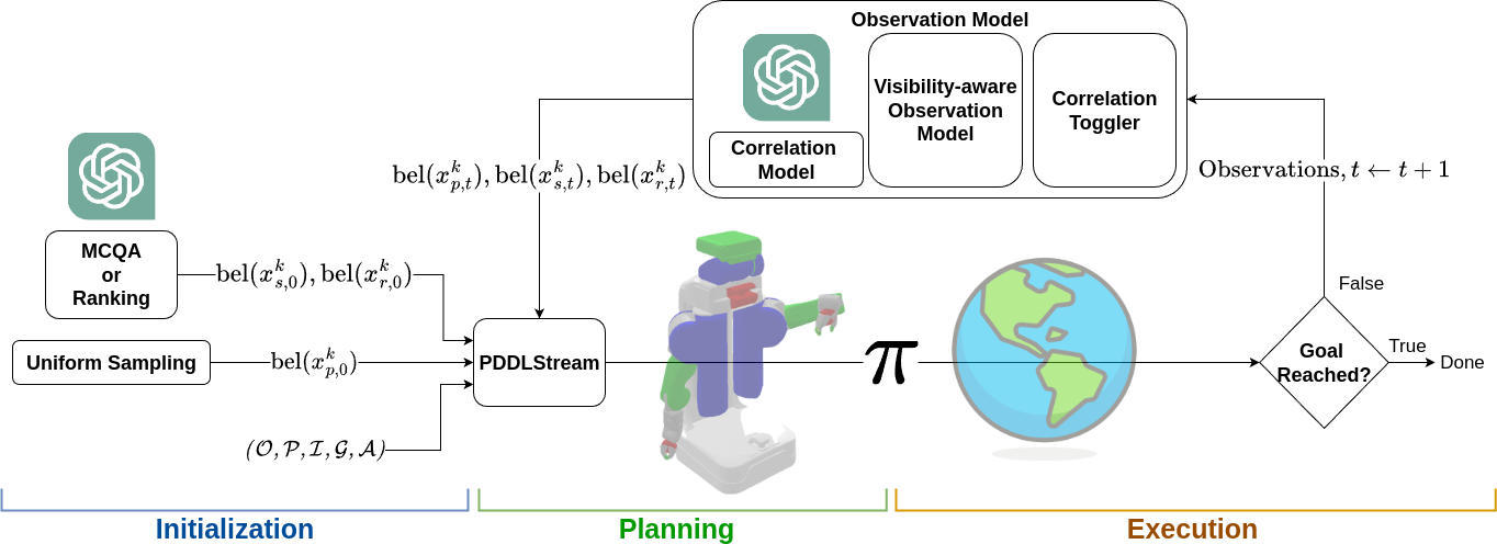
First obtain semantic priors and uniform pose samples. Plan and execute; after an observation, estimate visibility, optionally transfer co-location evidence and update the hierarchical belief. Replan on execution failure until the goal is reached. Figure 1 retains the complete loop.
III-A Initial belief generation with LLMs
Room and surface names become single-letter multiple-choice answers. The next-token log scores for those answers are normalized with softmax, giving the initial categorical beliefs. The toaster prompt is retained below; the surface query uses the same structure.
These probabilities express the model’s preference among the supplied options. Calibration, option-order robustness and coverage of atypical placements are not established by the normalization itself.
Predict the location of a toaster.
(A) Kitchen
(B) Bathroom
(C) Livingroom
(D) Garage
Return the letter that represents the location:
III-B Object state estimation
The state belief factors into pose conditioned on surface/room, surface conditioned on room, and room. Pose uses a particle filter; categorical levels use discrete Bayes updates. Visibility in [0,1] measures the fraction of initially uniform surface particles covered by the current view.
The factorization assumes conditional independence of observations and stationary objects. It provides a tractable approximation, not an unrestricted joint posterior over all object relationships.
Equation
III-B 1 Estimating object’s semantic location
With stationary objects, the previous posterior becomes the prediction. Multiply it by a visibility-aware target likelihood and independent cross-object likelihood factors, then normalize. Surface coverage is the seen-particle fraction; room coverage aggregates those counts across surfaces.
For a true location, detection likelihood is (1−pfn)v and a miss has likelihood 1−v+vpfn. At an incorrect location, detection has likelihood pfpv and a miss 1−vpfp. Both error rates are fixed to 0.01. Thus a small visible fraction provides weak negative evidence.
The cross-object factorization follows correlational object search. Shared occluders and scene structure can correlate observations beyond the assumed conditioning; the paper does not validate this independence or calibrate the error rates.
Equations 1–7
| (1) | ||||
| (2) |
| (3) |
| (4) |
| (5) | |||
| (6) |
| (7) |
III-B 2 co-location model
Generate three sentences describing each object’s common uses, embed the concatenation and compute cosine similarity. For nonnegative similarity, interpolate between uniform room probability and the same-room delta; for negative similarity, interpolate toward the normalized different-room complement. The definitions and piecewise equation remain exact.
A detected banana can increase the apple belief nearby; a dissimilar object can decrease it. A separate GPT-4o Boolean query disables co-location for categories normally spread across a house. Semantic similarity is a heuristic relation, not a measured physical co-location frequency. The negative-similarity complement divides by R−1 and needs special handling when only one room is available.
Equations 8–9
| (8) |
| (9) |
III-B 3 Estimating object pose
A target detection weights particles by Gaussian distance to its observed pose. A miss retains occluded/out-of-view hypotheses and assigns zero weight to visible ones. If another object is detected, an exponential distance kernel interpolates between attraction and repulsion according to semantic similarity; λ controls the distance scale.
The exact Gaussian, missed-observation and similarity equations are preserved. The continuous miss rule hard-zeros visible particles despite the categorical model’s nonzero false-negative rate. Eq. (14) also includes the previous particle weight inside a quantity called a likelihood; how it combines with Eq. (12)’s prior should be distinguished from Algorithm 1’s direct weight assignment. No silently corrected formula is substituted.
Equations 10–15
| (10) | ||||
| (11) | ||||
| (12) |
| (13) |
| (14) |
| (15) |
IV Experiments
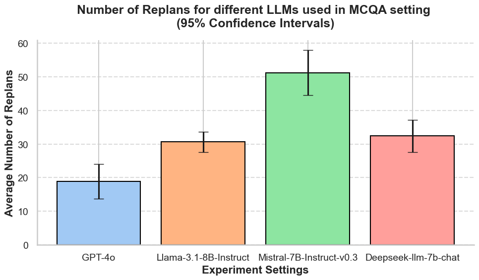
Experiments use Housekeep-derived geometric household simulations and Toyota’s HSR in a mock apartment. GPT-4o is selected after an MCQA comparison with smaller models and used for the remaining experiments. The embedding model, particle count, measurement σ and similarity-distance λ are not specified in this paper.
IV-A Large-scale simulations
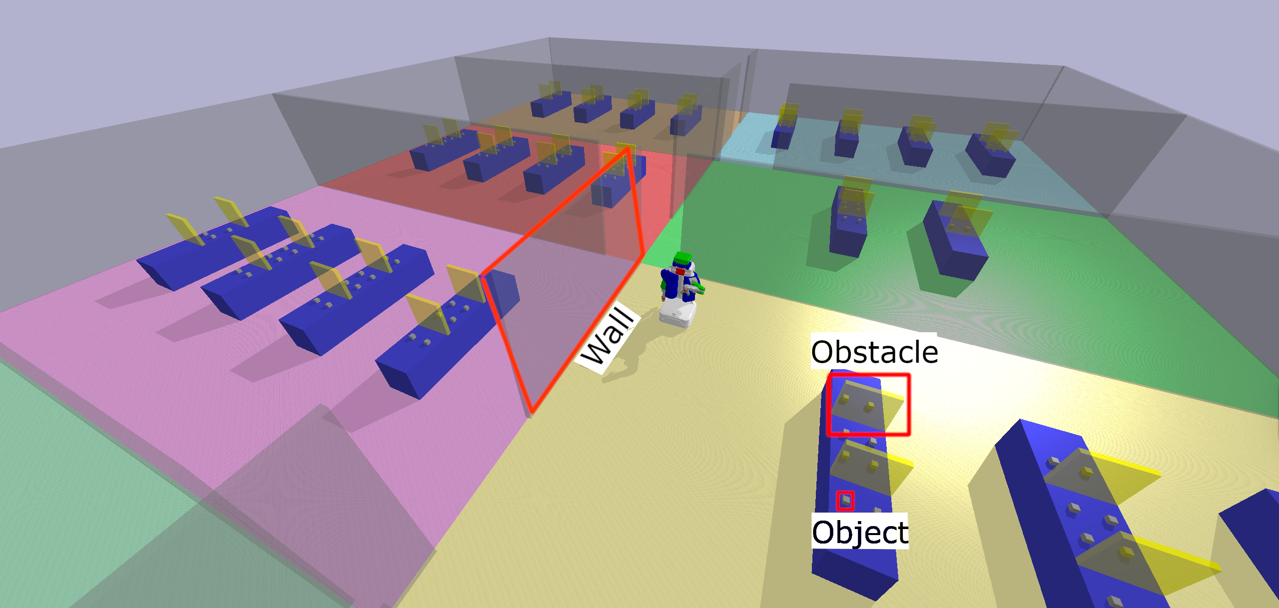
Housekeep human placement annotations determine room–surface–object sampling, reducing manual placement choices favorable to the method. Simulations use simple geometric boxes because the planner consumes semantic labels rather than visual semantics; this does not test end-to-end perception robustness.
IV-A 1 Comparative analysis
Six variants separate initialization and updates: uniform/Bayesian baseline; uniform plus co-location; uniform plus direct LLM belief updates (LGBU); MCQA priors alone; MCQA plus co-location; and MCQA plus LGBU. LGBU queries current belief, inspected location, visibility, detection result and co-detected objects, then normalizes answer-token probabilities.
Table I preserves the exact configurations. Its first row repeats the surface-belief symbol, while the caption identifies both room and surface priors; this is retained as a source notation discrepancy.
| Baseline | Co-Model | LGBU | MCQA | MCQA with Co-Model | MCQA with LGBU | |
|---|---|---|---|---|---|---|
| , | Uniform | Uniform | Uniform | MCQA | MCQA | MCQA |
| co-location model | No | Yes | No | No | Yes | No |
| LLM generated update | No | No | Yes | No | No | Yes |
| 4 rooms 8 surfs | 4 rooms 16 surfs | 6 rooms 12 surfs | 6 rooms 24 surfs | 8 rooms 16 surfs | 8 rooms 32 surfs | |
|---|---|---|---|---|---|---|
| Baseline | ||||||
| Co-Model | ||||||
| MCQA | ||||||
| MCQA with Co-Model | ||||||
| LGBU | ||||||
| MCQA with LGBU |
| 4 rooms 8 surfs | 4 rooms 16 surfs | 6 rooms 12 surfs | 6 rooms 24 surfs | 8 rooms 16 surfs | 8 rooms 32 surfs | |
|---|---|---|---|---|---|---|
| Baseline | ||||||
| Co-Model | ||||||
| MCQA | ||||||
| MCQA with Co-Model | ||||||
| LGBU | ||||||
| MCQA with LGBU |
IV-A 2 Comparison results
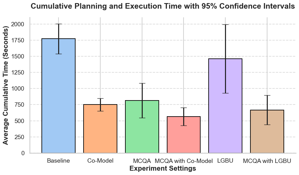
There are six layouts: 4/6/8 rooms, each with either two or four surfaces per room. Fifty environments per layout vary semantic labels and placements, with obstacles producing occlusions. Tables II–III report paired excess time/replans relative to the best method in each layout, with 95% confidence intervals. Zero means best in that comparison, not zero runtime or replanning.
At six rooms/twelve surfaces, the baseline takes 1,205.3±272.0 extra seconds and 17.2±5.4 extra replans; MCQA plus co-location is the reference best. Co-location alone adds 185.1±145.6 seconds and 5.5±3.1 replans. MCQA plus co-location is best by mean time in five layouts; co-location alone wins the largest layout, and several replan comparisons favor MCQA or tie with LGBU variants. The broad claim of uniformly lowest means/variability exceeds the tables.
Direct LGBU often underperforms Bayesian variants, but it is faster than the uninformed baseline in every tabled layout, so the blanket statement that it is worse than baseline on both metrics is too strong. In five adversarial layouts with randomized placements, Bayesian methods finish, while the caption reports LGBU and MCQA+LGBU hitting the 100-replan cap in three of five trials. This small stress test supports a limited robustness claim; it does not establish universal recovery from misleading priors.
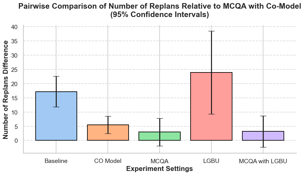
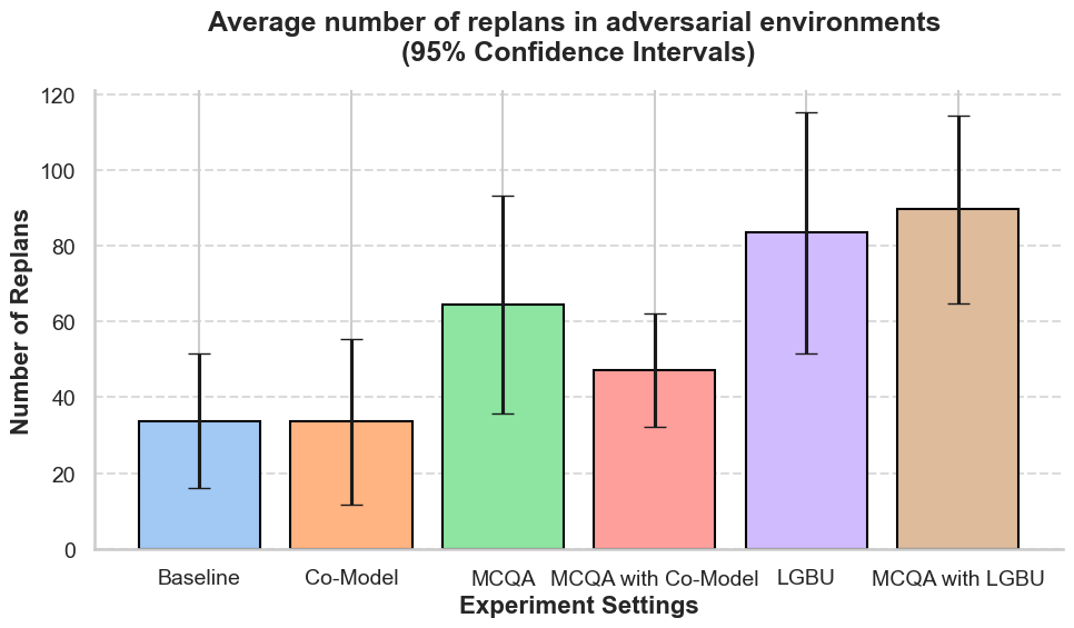
Note: The LGBU and MCQA with LGBU experiments had a total limit of 100 replans, which was exceeded 3 out of 5 times this experiment was run.
IV-B Real-world experiments
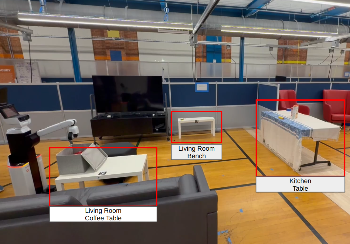
HSR moves an apple from the kitchen table to the living-room coffee table in a two-room, three-surface setup. A banana supplies positive semantic evidence, a screwdriver dissimilar evidence, and cereal/cracker boxes hide the target.
Reported planning/execution times are 365 s for baseline, 112 s with co-location, and 100 s with MCQA plus co-location: the last is 72.6% below baseline. This is one described scenario without repeated-trial uncertainty or a broad real-world success-rate evaluation.
V Related Work
Belief-space TAMP handles uncertainty but remains computationally demanding; object-search systems exploit observation structure without generally supplying a complete manipulation task model. CoCo-TAMP improves semantic belief estimation inside an existing planner.
Other LLM/TAMP work infers constraints, proposes plans, reasons about failures or translates language into PDDL. Here the LLM supplies placement priors and object relations; geometric planning and observations constrain execution. That distinction does not make every object-search system a formal special case of this implementation.
VI Conclusion
The combination of semantic priors and observation-grounded Bayesian updates improves search efficiency in the reported household tasks. Transfer to factories/hospitals and unknown room/surface layouts is untested. Dynamic objects, calibrated semantic uncertainty and reliable handling of atypical arrangements remain important boundaries.
ACKNOWLEDGMENT
The work acknowledges UT Austin LARG support from NSF, ONR, ARO, DARPA, Lockheed Martin and Good Systems. Peter Stone’s compensated Sony AI chief-scientist role was reviewed under UT Austin’s research-objectivity policy.
APPENDIX
The complete appendix supplies all prompts, the detect action and two PDDL streams, the belief factorization and surface equations, the particle-filter algorithm, dataset construction and the real-robot traces. These executable/formal examples remain intact.
VI-A Co-location Model Prompt
The three-sentence toaster example illustrates the text embedded for semantic similarity. The exact prompt and GPT-4o response are retained; this is a qualitative example, not evidence that cosine similarity is a calibrated location probability.
Equation
Prompt: Explain the common use of a toaster in three sentences.
LLM Response (GPT4o): A toaster is commonly used to toast slices of bread, making them crispy and golden brown. It’s also useful for heating up and adding a slight crunch to bagels, English muffins, and some pastries. Additionally, many people use a toaster to quickly prepare breakfast items like Pop-Tarts or frozen waffles.
VI-B Co-Location Toggler Prompt
The toggler asks whether a category is commonly distributed throughout a household, as with switches or doorknobs. A True/False response determines whether to suppress co-location transfer. The exact system/user prompts remain below.
Equation
System Prompt: You will be given an object that commonly appears in a typical household environment. Using common sense, determine if the object tends to be distributed throughout a typical household, such as doorknobs and light switches.
User Prompt: The following is the object: [object]
LLM Response (GPT4o): True / False
VI-C LGBU Prompt
LGBU receives the current belief, inspected location, coverage, detection result and other detected objects. It selects a likely location from supplied choices; answer-token probabilities become the updated belief. The exact structured prompts are retained for comparison with the explicit Bayesian update.
Equation
System Prompt: You will receive:
- •
Current belief about where an object might be located.
- •
observation_location: the location that was just inspected.
- •
visibility: how much of the location was visible. 0 means not visible at all, 1 means fully visible.
- •
result: whether the object was found there.
- •
co_detected: other objects found at the same location.
Based on this information and common sense, predict where the object is most likely to be now. Choose the most likely location from the given options.
User Prompt:
- •
Current belief about [object_name]: [belief_text]
- •
observation_location: [obs_loc]
- •
visibility: [visibility]
- •
result: [result]
- •
co_detected: [co_detected_text]
Given this information, where is object_name most likely to be? [options_text]
Similar to the MCQA method, the belief is updated using next token prediction, where [option_text] is a multiple choice with a character paired with a surface or room.
VI-D Detect action
detect requires typed object/surface/room arguments, the current robot base, a sampled object pose and a certified visibility configuration. Its effects assert the sampled pose/support and increase total cost. sample-PoseB certifies a sampled surface pose; inverse-visibility samples base/head configurations and a head trajectory whose viewing cone covers that pose.
All three original PDDL blocks are preserved exactly, including indentation. The explanatory prose repeats ?pb where the Vis predicate uses ?bq; the actual listing has ?bq. View-cone certification is distinct from successful perception through an occluder, which the execution/belief loop must handle.
(:action detect
 :param (?o ?s ?r ?pb ?bq ?hq ?ht)
 :pre (and (IsItem ?o) (IsSurf ?s) (IsRoom ?r)
           (AtBConf ?bq) (PoseB ?o ?pb ?s)
           (Vis ?o ?pb ?bq ?hq ?ht))
 :eff (and (Supported ?o ?pb ?s) (AtPoseB ?o ?pb)
           (increase (total-cost)
           (DetectCost ?o ?s ?r ?pb))))
(:stream sample-PoseB :inp (?o ?s) :dom (and (IsItem ?o) (IsSurf ?s)) :out (?pb) :cert (and (PoseB ?o ?pb ?s)))
(:stream inverse-visibility
:inp (?o ?pb ?s)
:dom (and (IsItem ?o) (IsSurf ?s) (PoseB ?o ?pb ?s))
:out (?hq ?ht ?bq)
:cert (and (Vis ?o ?pb ?bq ?hq ?ht)))
VI-E Object State Estimation Derivation
The derivation applies chain rules, conditional independence and a Markov simplification to separate pose, surface and room beliefs. It assumes that knowing an object’s room/surface removes extra semantic-observation information from pose estimation.
Equations (17)–(21) repeat the room variable in the pose-conditioning arguments where the preceding description requires room and surface. The final removal of history relies on the recursive belief retaining past evidence; it is not a generic consequence of state Markovity alone. The entire printed derivation is unchanged.
Equations 16–21
| (16) | ||||
| (17) | ||||
| (18) | ||||
| (19) | ||||
| (20) | ||||
| (21) |
VI-F Belief over Surfaces
Surface updates mirror room updates, conditioned additionally on the room: a target detection/miss likelihood times cross-object evidence, followed by normalization. The surface relation sums over possible room–surface locations of the other object. All six equations and the detected/not-detected cases are retained.
Equations 22–27
| (22) | ||||
| (23) |
| (24) |
| (25) |
| (26) |
| (27) |
VI-G Occlusion Aware Particle Filter Algorithm
Algorithm 1 keeps object poses stationary, weights by a target observation or an occlusion-aware miss, optionally multiplies in semantic-distance evidence from another detected object, then resamples N particles. Both the original PDF layout and copyable MathML version are retained. If all weights vanish, the displayed algorithm supplies no fallback.
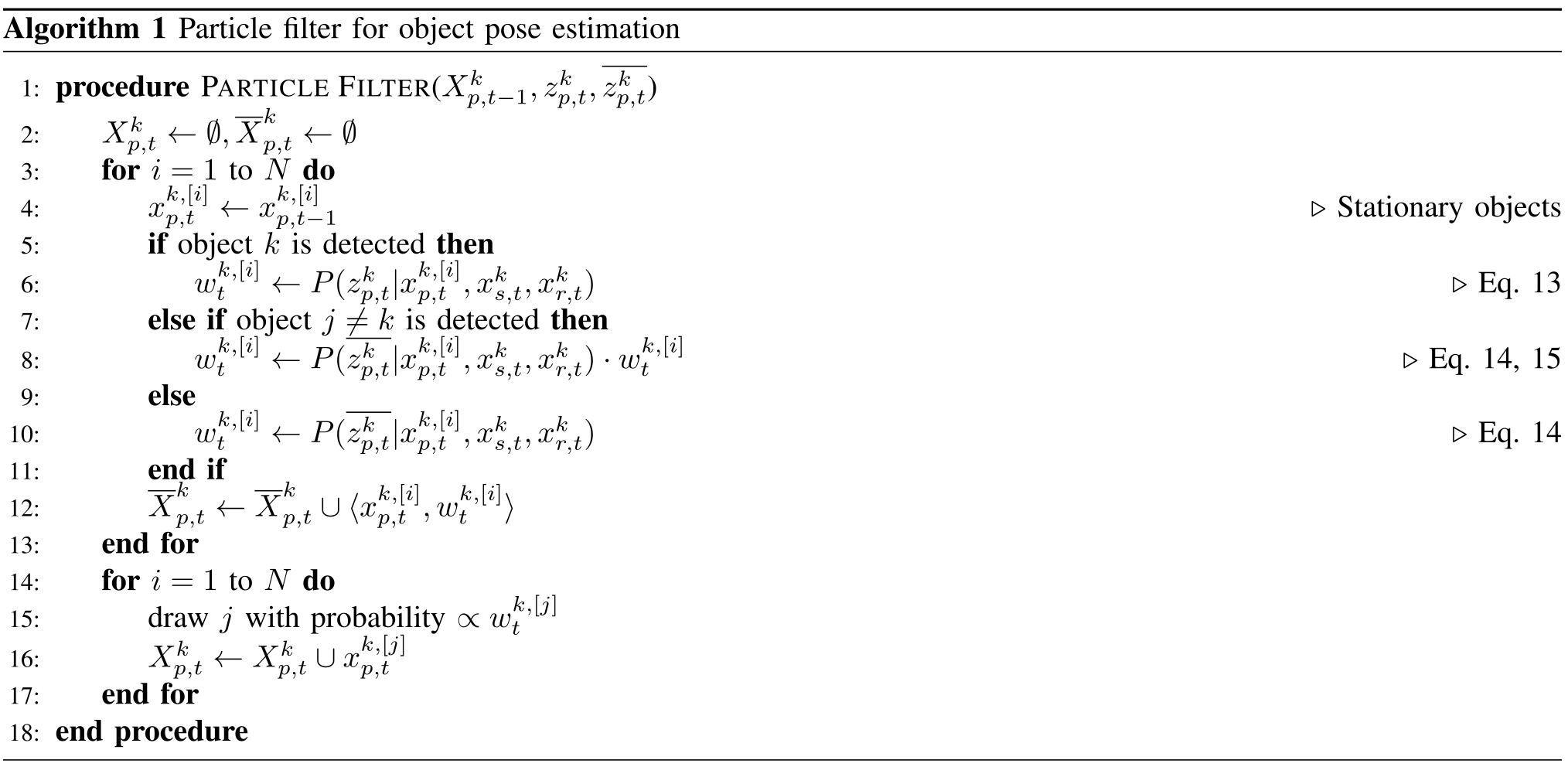
Copyable particle-filter algorithm
VI-H Simulation Environment Generation
Housekeep supplies 1,799 object categories, 585 surface types, 15 room types and 45,556 entries, with ten annotators ranking candidate placements. Correct placements score from N downward; incorrect placements from −N upward. Remove surfaces judged implausible by a majority, sum scores and normalize for sampling.
Rooms, surfaces and objects are sampled hierarchically to construct each environment. The exact multiport-hub ranking/scoring examples remain below. Mapping aggregate scores into [0,1] does not by itself specify normalization to a probability distribution; those details and annotation disagreement limit interpretation as calibrated placement likelihoods.
Object: multiport hub | Room: kitchen
Correct (ranked): carpet, fridge, table, counter, sink
Incorrect (ranked): chest, cooktop, microwave, dishwasher, stove
Implausible: oven, shelf, top cabinet, chair, bottom cabinet
Object: multiport hub | Room: kitchen
Correct: carpet=15, fridge=14, table=13, counter=12, sink=11
Incorrect: chest=-15, cooktop=-14, microwave=-13, dishwasher=-12, stove=-11
VII Real World Experiment Analysis
The baseline inspects coffee table, kitchen table, bench, coffee table and kitchen table, requiring four replans. Co-location alone needs three inspections/two replans: after seeing the banana behind the first failed kitchen view, it retries that table from another view. MCQA plus co-location starts at the kitchen table and needs two inspections/one replan.
The initial/goal literals and all three exact execution traces are retained. Failed kitchen observations arise from the cracker/cereal occluders; other failures inspect the wrong surface. The demonstration separates prior-guided first choice from co-location-guided persistence after occlusion.
Initial literal:
(IsItem ?apple),(IsItem ?banana),(IsItem ?cracker_box),
(IsItem ?cereal_box),(IsItem ?screwdriver),
(IsSurf ?coffee_table),(IsSurf ?bench),(IsSurf ?table),
(IsRoom ?living_room),(IsRoom ?kitchen),
(HandEmpty ?arm), (AtBConf ?start)
Goal literal:
(At ?apple ?coffee_table)
Baseline:
detect ?apple ?coffee_table ?living_room (1)
detect ?apple ?table ?kitchen            (2)
detect ?apple ?bench ?living_room        (3)
detect ?apple ?coffee_table ?living_room (4)
detect ?apple ?table ?kitchen            (5)
Num of Replan: 4
Co-Model:
detect ?apple ?coffee_table ?living_room (1)
detect ?apple ?table ?kitchen            (2)
detect ?apple ?table ?kitchen            (3)
Num of Replan: 2
MCQA with Co-Model:
detect ?apple ?table ?kitchen (1)
detect ?apple ?table ?kitchen (2)
Num of Replan: 1