Overview
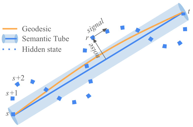
Intuition: adding a phrase to a sentence changes its meaning in context. Semantic Tube Prediction encourages hidden-state changes across related spans to point in consistent directions, while retaining next-token training. It aims to improve data efficiency without requiring the explicitly paired views used by LLM-JEPA. The geometric and stochastic descriptions are modeling hypotheses; the measured sixteen-fold data comparison is a specific regular-expression experiment with rescaled training epochs.
At a glance
STP regularizes the trajectory of language-model hidden states using a local straightness assumption. The ordinary language loss remains essential for generation. The study reports better accuracy and a large reduction in distinct training examples on a synthetic regular-expression task, plus experiments on other datasets and model families. Its results should be read as changing a particular training recipe, not disproving an immutable law of all language-model scaling.
1 Introduction
Scaling curves describe measured behavior under a training setup. The paper asks whether a more informative objective can move that curve. Its proposed geometric prior encourages related hidden-state increments to align within a semantic tube. This creates three separate claims to assess: the plausibility of the representation model, the behavior of the implemented regularizer, and the observed accuracy–data tradeoff. The last does not automatically prove the first.
Equation
2 Training and Inference Dynamics
The theory describes training trajectories and autoregressive inference using differential-equation analogies. These provide intuition for accumulated error, but their assumptions need to remain visible when connecting them to finite trained language models.
2.1 Training ODE
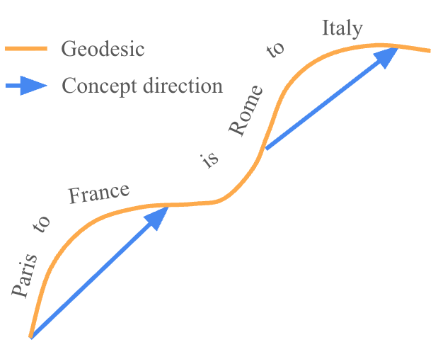
The construction rewrites token-conditioned hidden-state evolution as a continuous-time update after introducing a lifting function and related operators. This makes local direction and trajectory language available for the theory. It is a mathematical representation of the model under the stated construction, not evidence that an actual tokenizer produces a smooth semantic manifold.
Equations 1–2
| (1) | ||||
| (2) |
2.2 Mode Collapse at Inference Time
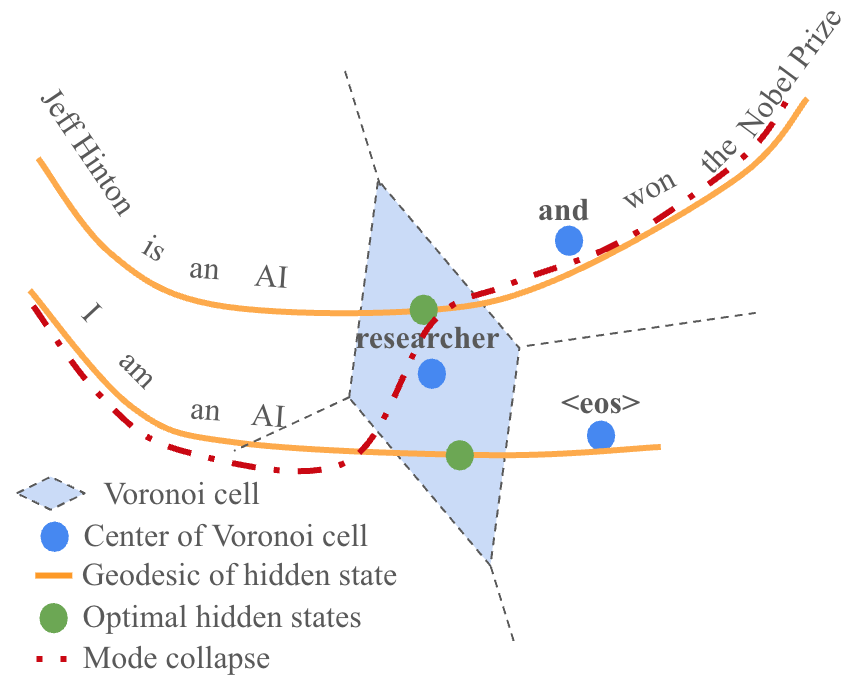
At inference, generated tokens feed back into future predictions, so errors can propagate differently from teacher-forced training. The paper models that accumulation as a stochastic perturbation and uses trajectory collisions to motivate loss of output diversity. The Gaussian and infinite-width arguments are approximations; they do not establish that every finite trained model follows the stated stochastic process.
Equation 3
| (3) |
3 Semantic Tube Prediction
STP turns the geometric motivation into an auxiliary training objective. The practical objective and its empirical ablations can be evaluated even when the strongest geometric interpretation remains unverified.
3.1 Semantic Tube
The objective compares contextual hidden-state differences for sampled spans and encourages compatible directions. Its tube interpretation permits a neighborhood around a proposed semantic path rather than demanding identical token sequences. The source’s lemma and theorem are retained with their assumptions. A small regularization weight matters because exact straightness need not hold for real language, and next-token prediction still supplies the generative objective.
Definition 3.1 (Local Linearity).
A time-indexed trajectory is defined as locally linear if such that for any time indices satisfying , we have:
Equation 4
| (4) |
where denotes the component of vector that is perpendicular to vector .
Lemma 3.2 (Straightening Lemma).
If , , and for all satisfying , then
Equation
Theorem 3.3 (Semantic Tube).
If is locally linear and for all satisfying , , then
Equation
Corollary 3.4 (Random Tube).
For randomly selected , if , then for any ,
Equation
3.2 Practical Considerations
The implementation chooses span boundaries and reuses hidden states already computed for ordinary training. This avoids a separate predictor or explicit pair of independently encoded views. Low extra arithmetic is a property of this implementation; it should be distinguished from the additional passes required by the earlier LLM-JEPA method.
3.3 Related Work
The related-work discussion connects manifold hypotheses, local linearity, representation learning and language objectives. These connections motivate the construction but do not make its assumptions consequences of all earlier theories. The important comparison is what information each objective requires and which aspect of a representation it constrains.
4 Experiments
Experiments test loss behavior, accuracy, data requirements, representation diversity and design sensitivity. Those measurements provide complementary evidence. Improvements in several proxies should not be treated as direct measurements of an otherwise unobserved semantic signal-to-noise ratio.
4.1 Loss Landscape
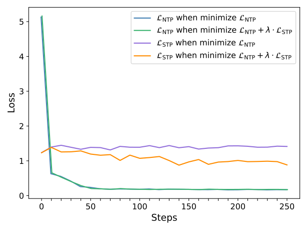
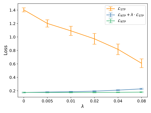
The monitored objectives show that optimizing the generative term does not automatically optimize the geometric term. Increasing regularization smooths the measured trajectory statistic over the tested range while token loss changes less. The strongest reduction in that statistic need not coincide with the best accuracy, so smoothness is a design target rather than a complete performance metric.
4.2 Better Accuracy
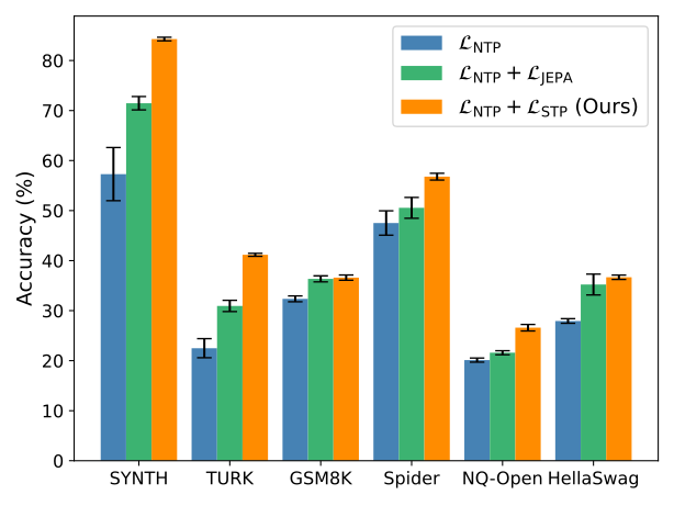
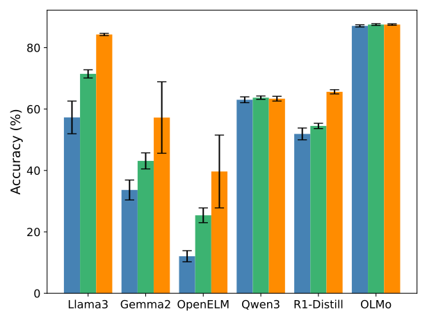
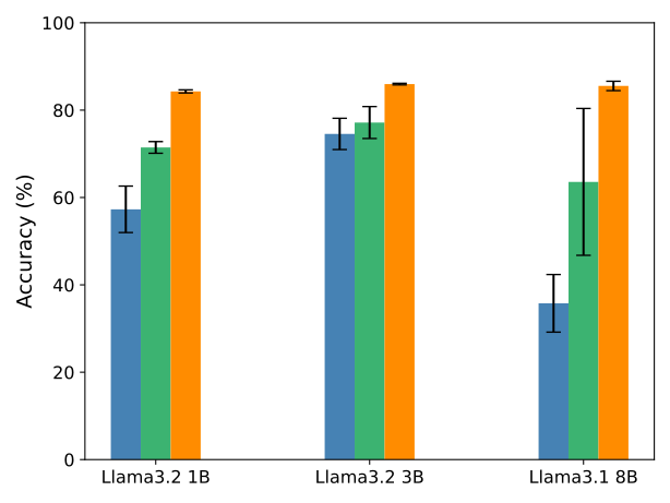
The comparisons cover regular-expression generation, question answering, mathematical problems, SQL and multiple-choice completion, with several model families and sizes. Accuracy improves across the reported experiments. Their evaluation rules differ by task, and successful adaptation of a pretrained model should not be described as evidence of broad pretraining from scratch.
4.3 Data Efficiency
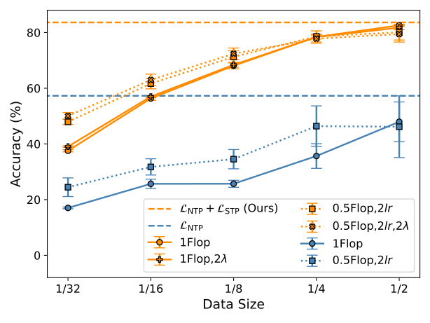
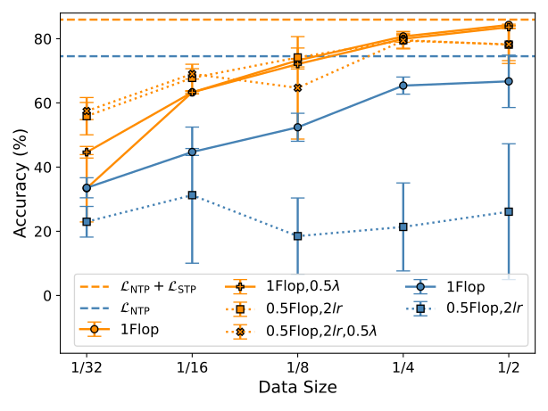
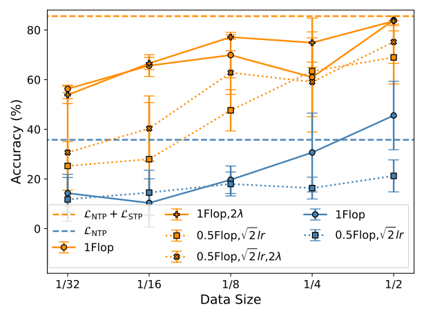
The headline data-efficiency experiment reduces the number of distinct NL-RX-SYNTH examples while increasing training epochs proportionally. STP can match a full-data baseline using one-sixteenth of the examples in the reported setting. Because update exposure is compensated, this is not a sixteen-fold reduction in training compute. The result is a benchmark-specific shift in a training curve, not a contradiction of every empirical scaling fit.
4.4 Preserving Diversity
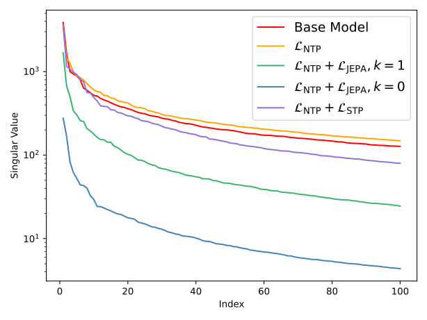
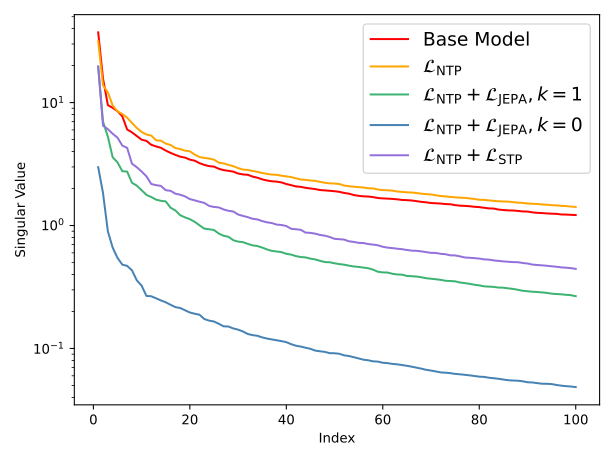
The diversity analysis examines two functionally equivalent regular-expression endings with different frequencies. STP retains both patterns better in this test, and normalized versus unnormalized singular spectra suggest different directional and magnitude structure. These are concrete dataset preferences and representation diagnostics; they do not certify preservation of all useful linguistic diversity.
| Suffix | Semantic Tube | Regular | LLM-JEPA |
|---|---|---|---|
| .* | 88.5% | 29.9% | 68.9% |
| .*.* | 68.0% | 28.0% | 32.0% |
4.5 Tuning λ
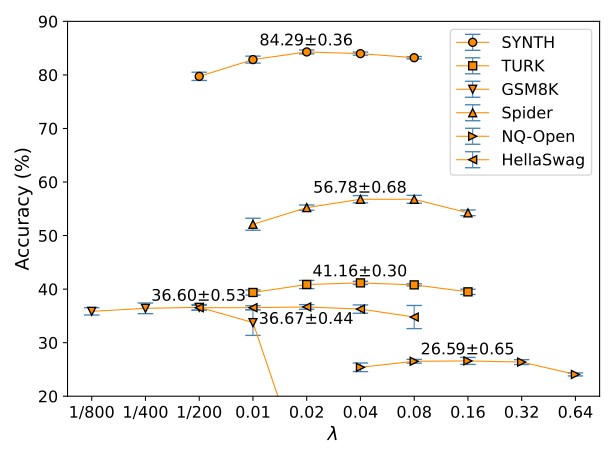
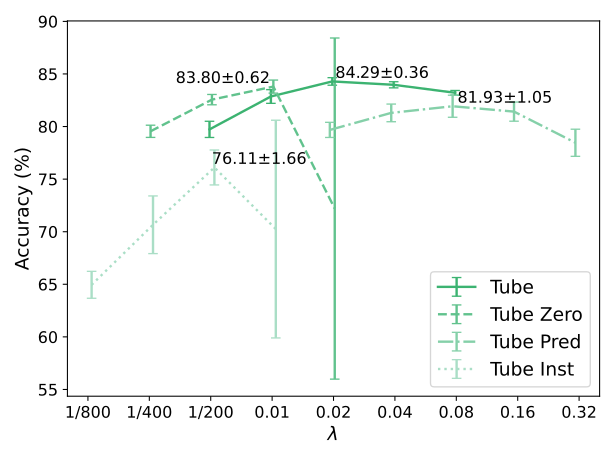
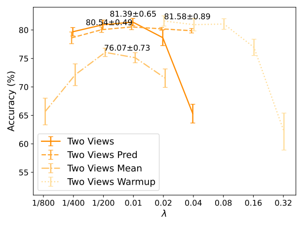
Accuracy varies non-monotonically with the auxiliary-loss weight. A useful range appears across the tested configurations, while excessive regularization can hurt. This supports tuning a modest geometric constraint alongside the token objective rather than trying to enforce perfect straightness.
4.6 Ablation
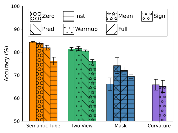
Ablations change span boundaries, add a predictor, use explicit paired views, mask spans and compare curvature objectives. The original formulation performs best among the tested alternatives. An auxiliary linear projector can degrade performance, illustrating that an added predictor is not automatically beneficial in a regularizer that reuses the model’s own hidden states.
5 Conclusion
The empirical contribution is a low-overhead auxiliary loss with promising task-specific data efficiency. The broad statements about least action, universal semantic geometry and scaling require more than these experiments establish. A useful engineering reading separates the implementable loss and controlled results from the proposed explanation of why they work.
Impact Statement
The source gives a general impact statement without a task-specific risk analysis. It should not be read as evidence that changing a language-model objective removes the usual downstream reliability or misuse concerns.
Appendix A Training ODE
The appendix derives the continuous-time training representation by defining a lifted update and an operator that reproduces the token-sequence evolution. Its operators and domain assumptions are part of the construction. A representation in ODE form alone does not validate a smooth semantic interpretation of the resulting states.
Equations
Appendix B Inference SDE
The inference model treats accumulated generation errors as Gaussian perturbations and motivates a stochastic differential equation using infinite-width results. Those idealizations should not be silently transferred to a finite, fully trained network. The exact proposition is retained so readers can check what assumptions carry the conclusion.
Appendix C Context-Aware Hidden State
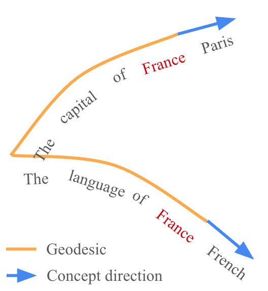
A hidden-state difference depends on the prefix that precedes a span. The same appended word can change meaning differently after different contexts. This explains why the implementation uses contextual increments rather than an embedding of the span in isolation.
Appendix D Proof of the Straightening Lemma
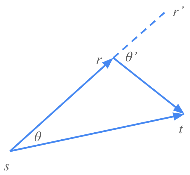
The straightening argument relates local geometric quantities under small-angle assumptions. The original formal statement and proof equations are preserved. Its approximation regime matters: a local calculation does not establish that long natural-language trajectories are globally straight.
Equation
Equations
Appendix E Proof of the Semantic Tube Theorem
The semantic-tube proof introduces auxiliary boundary tokens so the required endpoint conditions hold in the construction. Those boundary conditions are substantive assumptions. The theorem should be interpreted within that augmented mathematical setup rather than as an unconditional statement about arbitrary prompts.
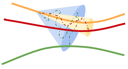
Appendix F Inference Cone
The inference-cone argument describes how a modeled random perturbation grows along a generated trajectory. Its Gaussian-process and tangent-kernel approximations restrict its scope. In particular, decreasing a bound involving a failure probability is not by itself a direct measurement or guarantee of lower realized mode-collapse probability in every finite model.
Proposition F.1 (Inference Cone).
The distortion between and behaves as a Gaussian process, where the scale of the deviation grows as
Equations
Appendix G Implementation Details
Implementation details explain how to sample boundaries, account for context and skip selected prompt or answer-choice regions. Using randomly selected boundaries differs from always fixing a question–answer split. The practical advice to use a small auxiliary weight reflects the possibility that real semantic paths are curved.
Equation
Appendix H Signal-to-Noise Ratio
This appendix relates conditional information, a Gaussian-channel approximation and data/accuracy bounds. The semantic signal and nuisance noise are not directly observed in the experiments. Consequently, higher measured accuracy or better sample efficiency does not uniquely identify an increased internal SNR; other changes can affect those outcomes. The exact assumptions and inequalities remain available for inspection.
Lemma H.1 (Data Efficiency).
Equation 5
| (5) |
Equations
Corollary H.2 (Signal-to-Noise Ratio).
Equation 6
| (6) |
Equations 7
| (7) |
Corollary H.3 (Accuracy).
Equation 8
| (8) |
Appendix I Data Efficiency
Additional data-subset curves repeat the analysis at larger tested model sizes. As in the main experiment, reducing distinct examples is paired with an altered epoch schedule. Keep the data axis, number of updates and model size separate when interpreting the comparison.
Appendix J Regular Expression Samples
The examples show two equivalent regular-expression endings used to probe preservation of dataset-specific variation. The table makes the preference distinction explicit but is not an evaluation of unrestricted linguistic creativity or diversity.
| Regular Expressions |
|---|
| .*([a-z])([AEIOUaeiou])([A-Za-z]).* |
| .*([A-Za-z]).*([0-9]).*.* |
| ((dog)(.*)).*([AEIOUaeiou]).* |
| (dog).*((truck)([A-Z])([0-9])).* |
| .*(.)&([0-9])&(dog).* |
| .*(dog).*((.)*).*.* |
| .*dog.*[a-z].*.* |
Appendix K Tuning λ
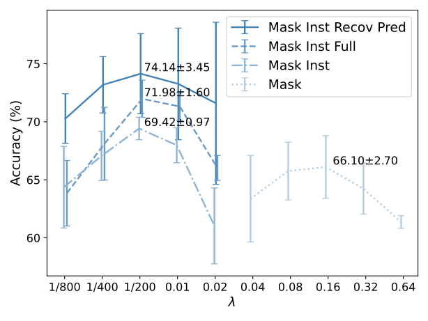
The extended loss-weight sweeps cover the alternative formulations. Some settings show sharp accuracy declines and higher run-to-run variation beyond the useful range. These plots expose sensitivity that an isolated best-number comparison would hide.
Appendix L Ablation
The complete ablations distinguish geometric span matching, explicit two-view supervision, masked-span recovery and curvature penalties. They test predictor additions, instruction handling and boundary choices. Keeping the alternatives separate helps identify what information each variant uses; the statistical comparisons apply to the tested configurations rather than every possible implementation.
| Two View | Mask | Curvature | |
|---|---|---|---|
| LLM-JEPA2 | 1.14e-3 | 1.77e-3 | 3.04e-5 |
| Two View | 4.76e-3 | 5.10e-5 | |
| Mask | 1.28e-4 |
| Zero | Pred | Inst | 2View | Pred | Mean | ||
| LLM-JEPA2 | 2.03e-3 | 2.34e-4 | 2View+Warmup | 0.0426 | 9.16e-6 | ||
| +Zero | 0.0185 | 5.56e-4 | 2View | 1.19e-6 | |||
| +Pred | 2.97e-4 | +Pred | 2.78e-4 | ||||
| Inst,Recov | Inst | Mask | Signed | ||||
| Mask+all | 0.0159 | 4.02e-3 | |||||
| -Pred | 2.34e-3 | 1.18e-3 | Curvature | 0.0368 | |||
| -Recov,Pred | 0.0103 |