Overview
The agent learns during a deployment episode: propose several actions, predict their usefulness, execute one, then revisit earlier decisions using actual outcomes. Its external evaluator stays frozen while the action generator and internal evaluator adapt.
At a glance
Reflective Test-Time Planning couples best-of-N action selection with parameter updates driven by verbal feedback and hindsight scores. On the authors’ household benchmark, mean category success rises from 10.4% without either reflection mechanism to 33.65%. Cupboard fitting and limited sim-to-real tests also improve, although fitting any compartment and reaching the correct compartment give different rankings.
1 Introduction
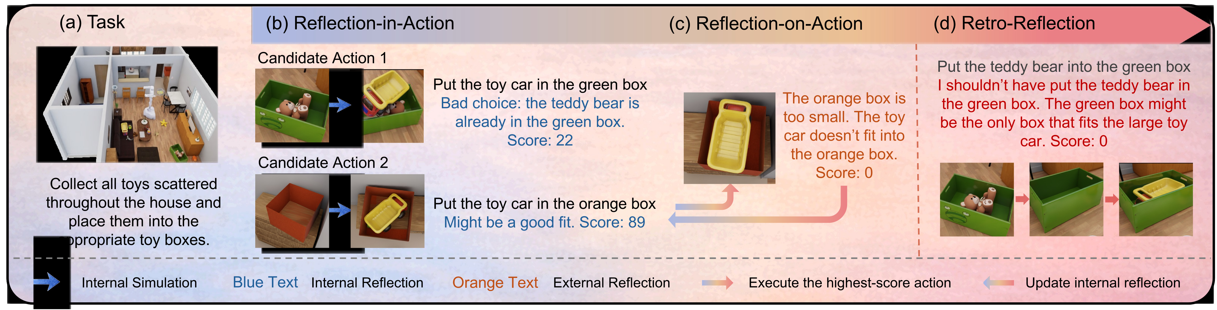
A physically successful action can still be strategically wrong: placing a small object may occupy the only space for a larger one. Immediate feedback diagnoses the local outcome; retrospective reflection revises earlier scores after downstream consequences become visible. The mechanism operationalizes reflective practice and double-loop learning by changing both decisions and the evaluator that guides them.
This edition covers all 33 pages of arXiv v3, dated 25 May 2026. It retains eight numbered figures, 18 numbered tables, 13 numbered equations, six additional displays including four training schemas, Algorithm 1 and all 46 references. The catalog’s original posting date remains distinct from the edition’s source version.
2 Related Works
Unlike Reflexion and Self-Refine, which primarily reuse critiques as context, this method turns hindsight feedback into deployment-time weight updates. Unlike fixed predictive scorers, it updates the internal evaluator after encountering failures. LoRA makes these updates smaller; spatial memory and 3D grounding provide the observations on which they depend.
The paper contrasts its single-episode adaptation with conventional planning and reinforcement-learning training loops. That comparison motivates this implementation; it does not establish that all planning or reinforcement-learning methods must keep their models fixed at deployment.
3 Reflective Test-Time Planning
Initialize a unified embodied model through supervised fine-tuning, then instantiate three copies: action policy π, internal evaluator Vᵢ and frozen external evaluator Vₑ. Action execution supplies new observations and a binary outcome signal. The learning signal is self-generated language grounded in that feedback, not an independent human reward oracle.
3.1 Reflection-in-Action
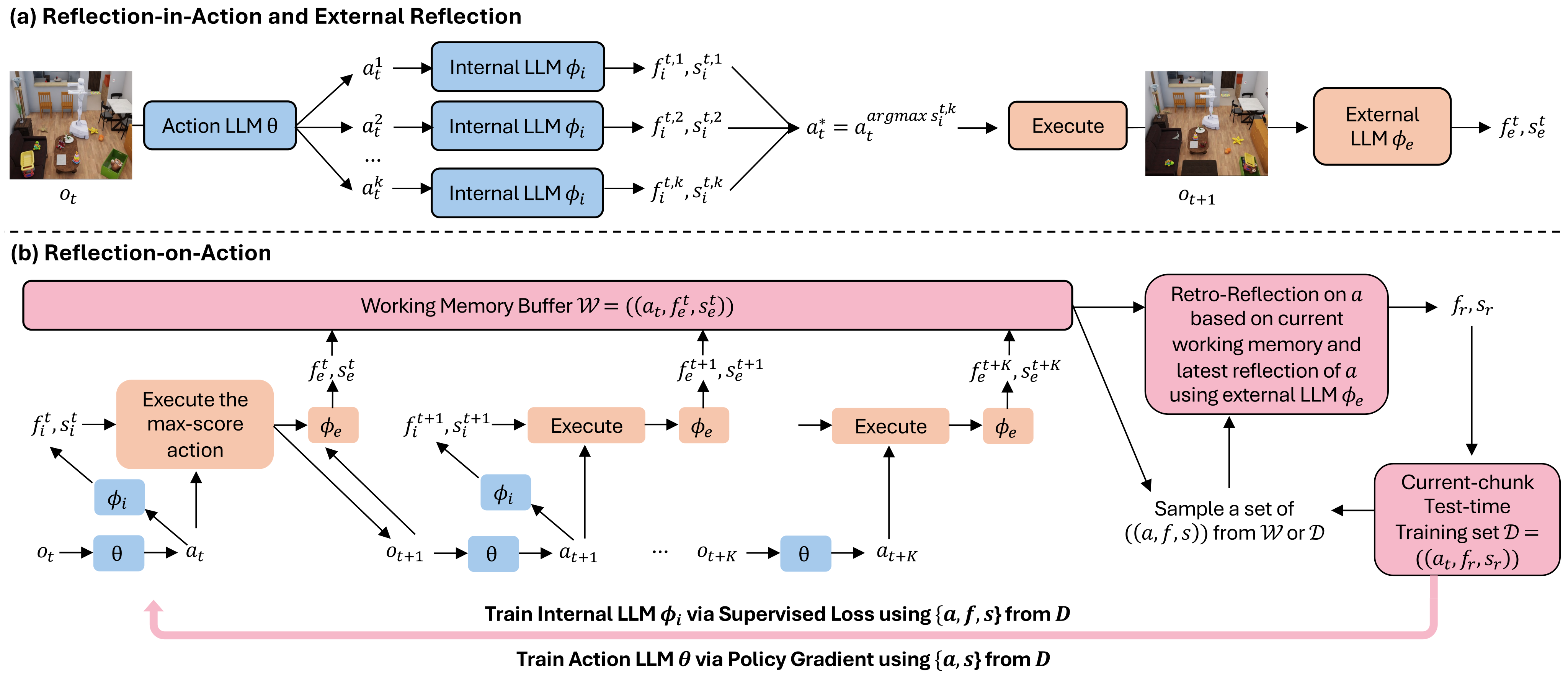
Construct a prompt from the task, current observation, previous action and previous external reflection. Sample N candidates at elevated temperature; score each with an internal reflection and a number from 0 to 100; execute the maximum-score candidate. Equations 1–4 contrast greedy decoding with this selection process. The internal “simulation” is model reasoning, not a verified rollout of physical dynamics.
Original selectable source
Equations 1–4
| (1) |
| (2) |
| (3) |
| (4) |
3.2 Reflection-on-Action
Execution can falsify a persuasive internal prediction. Post-action observations and success/failure feedback therefore support retrospective supervision for both the evaluator and policy. Only those two models update; the external teacher remains fixed.
3.2.1 Multi-Scale External Reflection
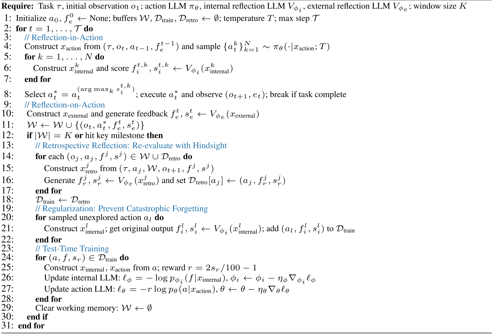
After each action, Vₑ describes what happened and assigns an immediate score. Accumulate recent transitions in a working buffer. At a milestone, such as leaving a room, or at K steps, re-evaluate earlier actions using the current window, latest observation and previous reflection. Store the newest hindsight assessment for each historical action; older actions may be subsampled as memory grows.
Equations 5–6
| (5) |
| (6) |
3.2.2 Test-Time Training Dataset Construction.
Training mixes hindsight-supervised action/reflection/score triples with randomly sampled unexplored actions labeled by the internal model’s current predictions. The second group anchors behavior outside the recent trajectory; the household implementation uses a 50:50 mixture. These are self-distillation targets, not newly observed outcomes for unexplored actions.
Equations 7–8
| (7) |
| (8) |
3.2.3 Test-Time Training
Train Vᵢ by negative log-likelihood of retrospective reflection text. Train π with a REINFORCE-style token-sequence loss, converting score s to reward 2s/100−1. Positive rewards increase the sampled action’s likelihood; negative rewards decrease it. Algorithm 1 includes both retrospective and regularization examples in the updates, then clears the short working buffer while retaining retrospective memory.
The displayed evaluator loss predicts f rather than an explicitly separate scalar-score loss. Scoring and repeated updates depend on the teacher’s calibration; the paper gives no general convergence, unbiased-policy-gradient or safe-adaptation guarantee.
Equations 9–13
| (9) |
| (10) |
| (11) |
| (12) |
| (13) |
4 Experiments on Long-Horizon Household Tasks
The household benchmark deliberately stresses mistakes whose consequences span rooms and actions. Its reported averages are unweighted means of four category percentages, not an explicitly reported overall task-weighted success rate.
4.1 Long-Horizon Household Task Construction
Build tasks on BEHAVIOR-1K scenes: Fitting tests geometry/capacity, Selection tests preferences and exploration, Preparation tests ordering constraints, and Hybrid combines them. GPT-5 receives complete scene graphs and proposes tasks, placements, trajectories and reflection scores across 3–7 rooms. Execute generated trajectories in OmniGibson and reject contradictory outcomes.
A shared LLaVA-3D model learns action and reflection formats before its three deployment copies are separated. Evaluation uses disjoint descriptions, scene configurations, placements and trajectories. Appendix P defines a 30-action budget and requires spatial, preference and ordering constraints as well as final object placement.

Original selectable source
| Baselines | Reflective Test-Time Planning Ablations | |||||||||||
|---|---|---|---|---|---|---|---|---|---|---|---|---|
| Reflexion | Self-Refine | ReflectVLM | PPO | DreamerV3 | 3DLLM-Mem | w/o RIA/ROA | w/o RIA | w/o ROA | w/o Act. | w/o Int. | Ours | |
| Fitting | 8.51% | 10.6% | 2.12% | 0% | 4.26% | 10.6% | 0% | 33.5% | 6.38% | 25.5% | 12.8% | 44.7% |
| Selection | 8.82% | 11.8% | 5.88% | 2.94% | 11.8% | 14.7% | 17.6% | 5.88% | 11.8% | 26.5% | 8.82% | 32.4% |
| Preparation | 15.9% | 12.7% | 14.3% | 7.94% | 11.1% | 9.52% | 11.1% | 3.17% | 19.0% | 20.6% | 17.5% | 31.7% |
| Hybrid | 6.45% | 9.68% | 6.45% | 3.23% | 12.9% | 9.68% | 12.9% | 3.23% | 12.9% | 16.1% | 9.68% | 25.8% |
| Average | 9.92% | 11.20% | 7.19% | 3.53% | 10.02% | 11.13% | 10.40% | 11.45% | 12.52% | 22.18% | 12.20% | 33.65% |
| #Data | 1 Epoch | 2 Epoch | 3 Epoch | w/o RIA/ROA |
|---|---|---|---|---|
| 25% | 15.6 | 20.3 | 22.1 | 1.3 |
| 50% | 18.7 | 24.8 | 19.6 | 4.4 |
| 100% (Ours) | 33.6 | 20.7 | 16.1 | 10.4 |
| 200% | 24.5 | 19.6 | 9.1 | 13.4 |
| 300% | 20.7 | 17.5 | 7.5 | 15.9 |
| Method | Fit | Sel. | Prep. | Hyb. | Avg. | Overhead |
|---|---|---|---|---|---|---|
| TTT on Ext. Refl. | 22.4 | 17.6 | 12.7 | 9.69 | 15.6 | 4 |
| TTT on Retro (Ours) | 44.7 | 32.4 | 31.7 | 25.8 | 33.7 | 1 |
4.2 Experimental Results & Analysis
Table 1 reports 33.65% mean success versus 11.20% for Self-Refine, 11.13% for 3DLLM-Mem and 10.40% without both reflection modes. Full category scores are 44.7/32.4/31.7/25.8% for fitting/selection/preparation/hybrid. Removing candidate reflection gives 11.45%; removing online training gives 12.52%; removing action-model or internal-model loss gives 22.18% or 12.20%. Both components help overall, but interactions differ by category.
SFT scaling peaks at the reported 100%-data/one-epoch setting, 33.6%; more epochs or data can reduce adaptation quality. Hindsight-based training gives 33.7% versus 15.6% for immediate-feedback training at roughly one quarter of its overhead. These ablations support the complete recipe; they do not establish that initialization supplies only formatting or that all reasoning is acquired during testing.
Transfer to 41 HM3D preparation tasks reaches 19.5% versus 7.32% for the strongest listed baseline. This is no additional domain-specific offline fine-tuning, but deployment-time updates still occur. No uncertainty intervals or repeated-seed protocol accompany these main comparisons.
Results Analysis.
Household success averages 33.65% across the four categories, with 44.7% fitting success. Removing either reflection component reduces the overall score, but some category interactions are non-monotonic. Thus the ablations support the combined recipe without proving that both mechanisms are indispensable in every task. HM3D transfer reaches 19.5% on 41 preparation tasks versus 7.32% for the strongest listed baseline. Training uses synthetic BEHAVIOR scenes, while deployment still includes online updates; no repeated-seed uncertainty accompanies these comparisons.
Necessity and Reliability of SFT Initialization and External LLM.
SFT initialization helps the system produce usable outputs, and the tested data/epoch settings show a peak followed by degradation. Initialization-only success is 10.4%, versus about 33.7% for the complete reflective system. These comparisons do not isolate initialization as format-only teaching or establish that every reasoning ability is acquired at test time. The frozen external teacher receives observed outcomes and simulator feedback. Human ratings support useful reflections but omit sample sizes, agreement and uncertainty. Immediate-feedback training reaches 15.6% at approximately four times the hindsight-training overhead, indicating that signal placement and credit assignment matter in this setup.
5 Experiments on the Cupboard Fitting Task
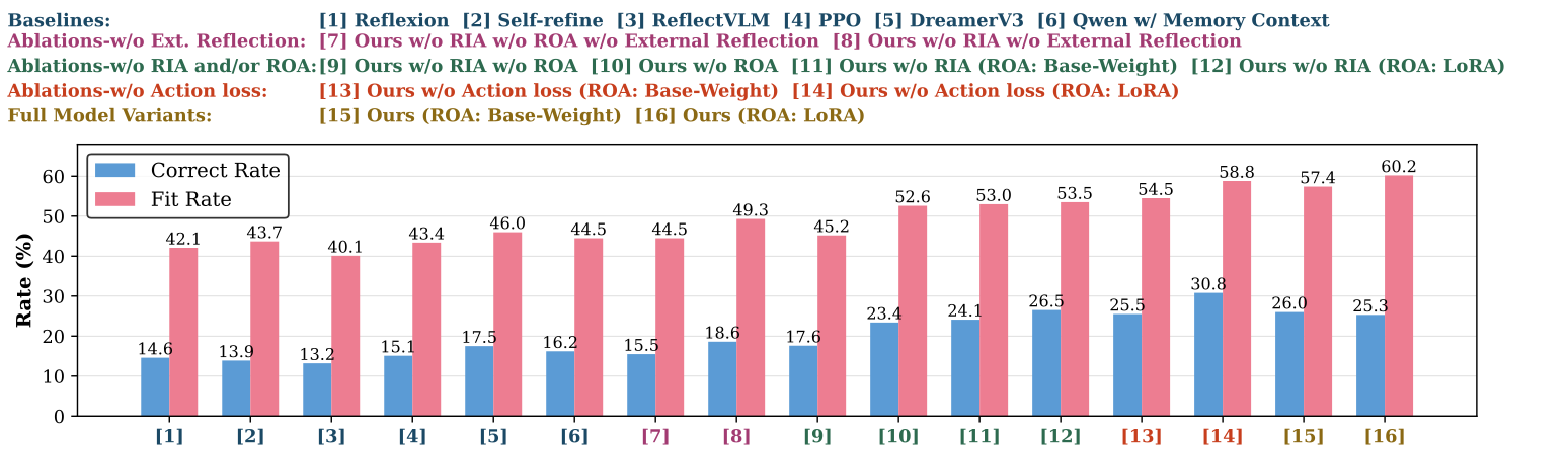
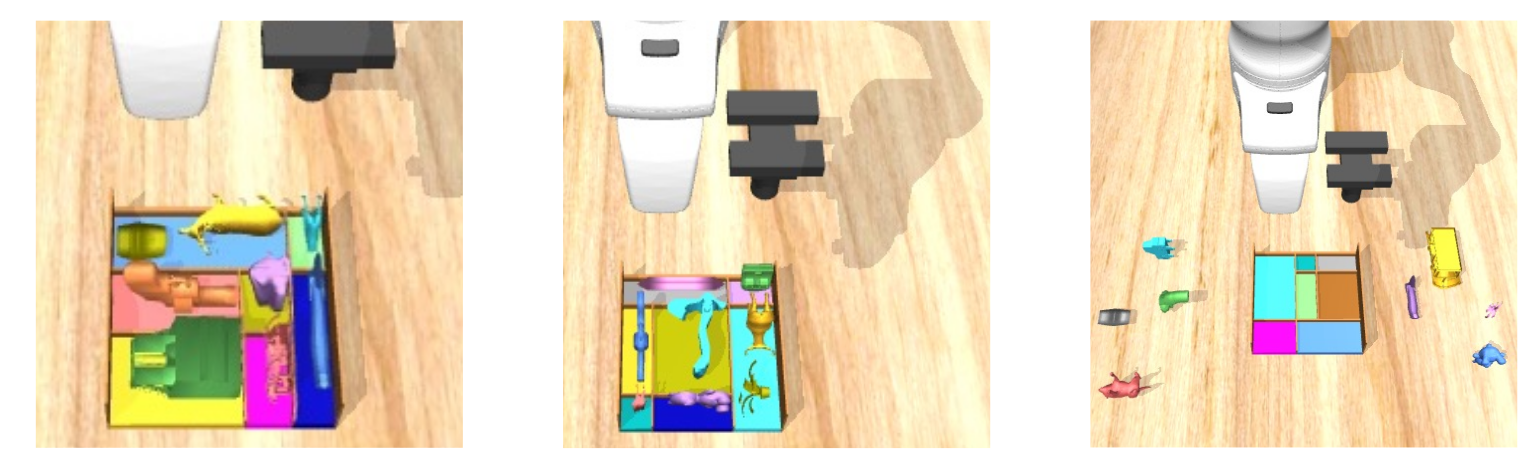
Cupboard Fitting uses MuJoCo, a Franka arm, colored objects and compartments with geometric constraints. Fit rate counts objects in any compartment; correct rate counts designated compartments. Full LoRA adaptation reaches 60.2% fit and 25.3% correct, versus 44.5/17.6% without either mode. Base-weight adaptation gives 57.4/26.0%.
The full model has the best fit rate, but not the best correct rate: the LoRA variant without action-model loss reaches 58.8% fit and 30.8% correct. Thus “improves both metrics” is true against basic baselines, not dominance over every ablation. Figure 3’s complete chart, absent from the HTML graphics, is restored from the PDF.
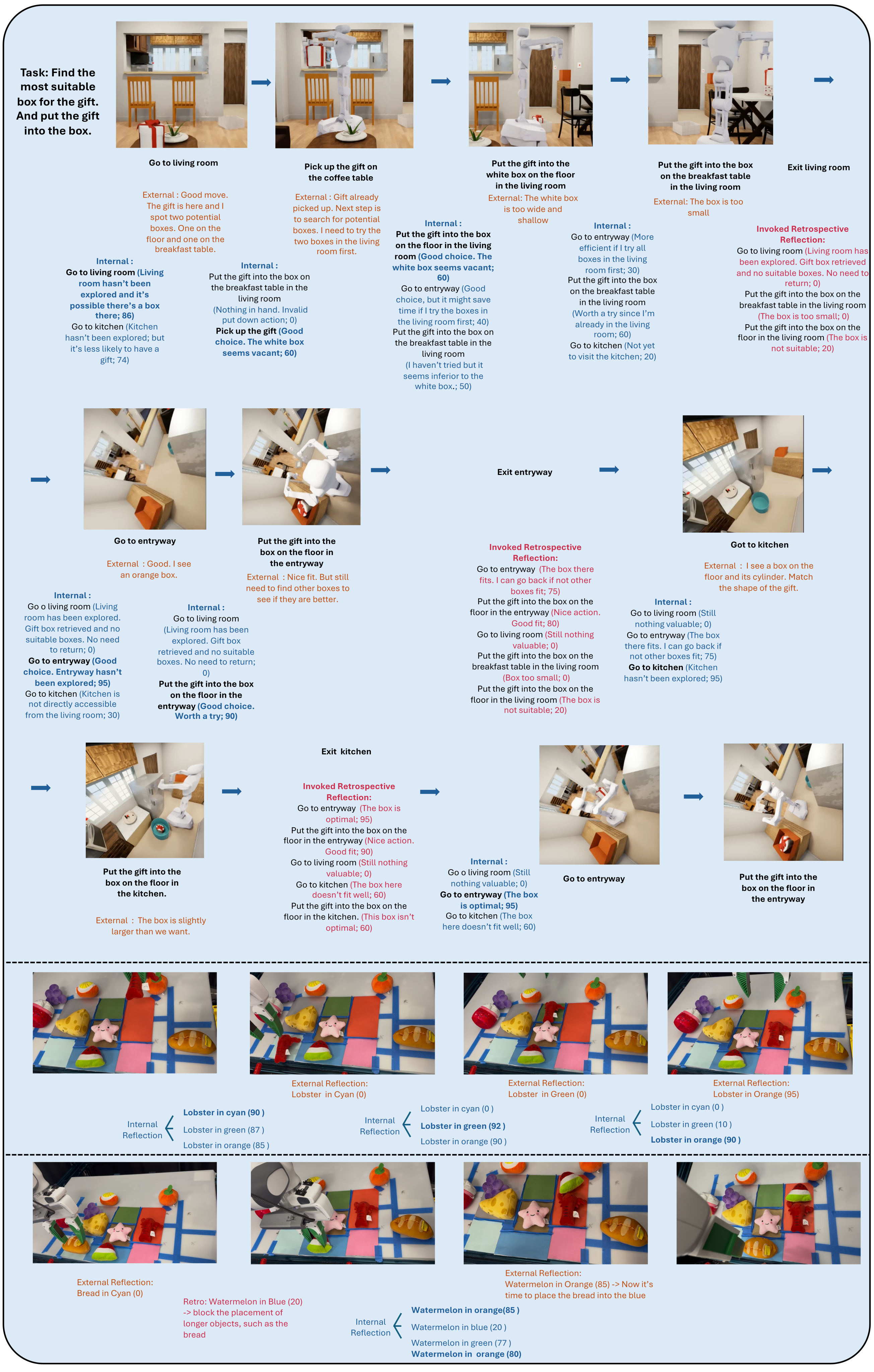
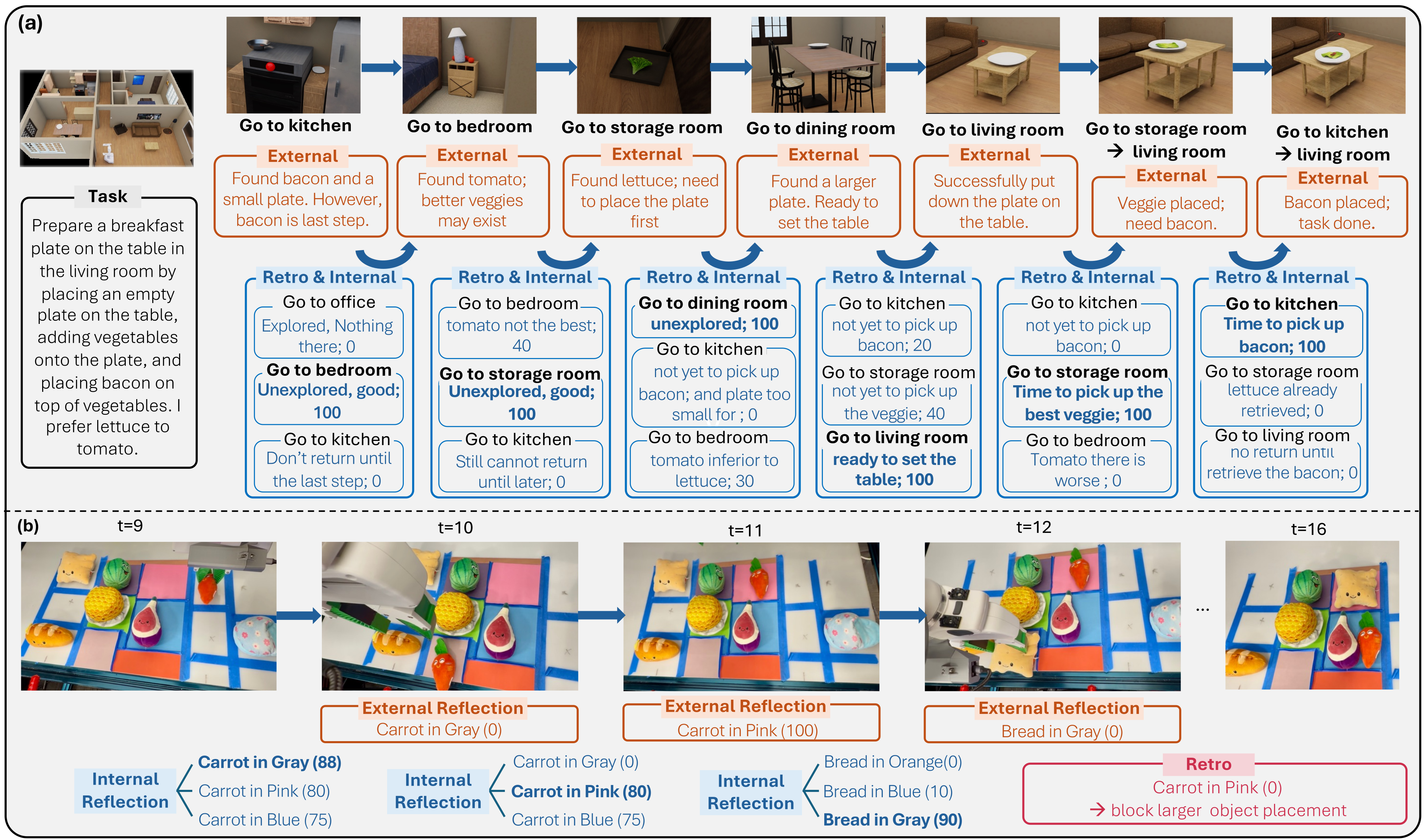
On the real Franka, direct sim-to-real transfer gives 40.6% fit/13.4% correct versus 13.1/4.5% without reflection. With real-domain fine-tuning, results are 44.2/16.6% versus 20.7/7.2%. “Zero-shot” permits online adaptation; real-task counts, fine-tuning data volume and statistical uncertainty are not specified. Figure 5 illustrates local corrections and later reassignment of blame.
Real-Robot Experiments.
On the real Franka, the full model reaches 40.6% fit and 13.4% correct placement without target-domain offline fine-tuning, versus 13.1% and 4.5% without reflection. After real-domain fine-tuning, the respective results are 44.2/16.6% and 20.7/7.2%. These object-level metrics support better performance in the tested setup, while missing trial counts and uncertainty limit stronger comparisons. Zero-shot transfer still permits online adaptation. Execution uses registered positions, structured grasp/place commands and bounds feedback rather than an end-to-end learned perception/control pipeline.
6 Conclusion
The evidence favors combining candidate selection, hindsight and online parameter updates on these constructed benchmarks. Remaining limits include imperfect external scoring, low absolute exact-placement rates, dependence on initialized formats and execution feedback, computational overhead and incomplete evaluation documentation. Tactile sensing is a proposed extension, not an evaluated capability.
Acknowledgments
Support includes ONR, Korea’s IITP/MSIT, Toyota Research Institute and Google’s academic compute program.
Appendix A Contribution Statement
Yining Hong is credited with the idea, implementation, data, experiments and writing; Huang Huang helped set up the physical robot; the remaining authors provided research guidance.
Appendix B Broader Impacts
The paper identifies possible benefits in failure recovery and risks from changing behavior during deployment, biased verbal assessments and reduced oversight. Interpretable reflections help inspection but do not themselves constrain adapted actions or prove safety.
Appendix C Test-Time Cost Analysis
The cost analyses distinguish extra reasoning and training time from environment interaction count. Their approximate ratios use different reference configurations, so they should not be combined without checking the denominator.
C.1 Computational Comparison
Average per-step wall time is reported as approximately three times the no-reflection baseline across the two benchmarks. Candidate generation/scoring and periodic updates create this cost. The paper does not provide absolute latency, hardware-normalized throughput or a complete end-to-end timing breakdown here.
Equation
C.2 Why the Overhead is Justified
The authors argue that fewer repeated mistakes can compensate for slower decisions and turn deployment time into learning. That is a task-dependent rationale; measured per-step overhead alone does not establish practical real-time control performance.
Deployment-Oriented Adaptation.
The additional computation occurs during deployment and can support adaptation to observed failures. This moves part of the learning cost from offline preparation to online operation. Whether that trade is practical depends on the task, hardware and allowable decision delay; the experiment does not establish general real-time control performance.
Reduction of Execution Waste.
Candidate reflection can reject poor actions before execution, while retrospective updates can reduce repeated failures. The reported comparisons show more successful task behavior despite slower decisions. They do not separately measure whether saved physical actions repay the full wall-clock, teacher-model and hardware cost in every deployment.
Conversion of Time into Learning.
Extra test-time computation updates the internal models instead of merely extending the action rollout. In Table 6, tripling the vanilla action budget gives 8.46% mean success versus 8.79% vanilla and 33.65% full. Its vanilla hybrid score differs from Table 1, so the two tables are not one identical baseline run. The result favors the tested reflective recipe under approximate budget matching; it does not prove that all alternative uses of test-time compute are inferior.
| w/o RIA w/o ROA | Ours (Full) | ||
|---|---|---|---|
| Vanilla | Same Time Budget | ||
| Fitting | 0.00% | 0.00% | 44.7% |
| Selection | 17.6% | 14.7% | 32.4% |
| Preparation | 11.1% | 12.7% | 31.7% |
| Hybrid | 6.45% | 6.45% | 25.8% |
| Average | 8.79% | 8.46% | 33.65% |
C.3 Compute-Matched Experiment
Tripling the vanilla action budget is an approximate time-matched comparison. Table 6 gives 8.79% vanilla, 8.46% expanded-budget and 33.65% full success. However, its vanilla hybrid score is 6.45%, whereas Table 1 lists 12.9%, yielding a different baseline average. Preserve both reported tables rather than treating them as one identical run.
Equation
Conclusion.
The paper reports roughly threefold per-step latency and better task performance than a vanilla policy with three times the action budget. This is an empirical comparison of the tested systems. The different nominal baselines and incomplete hardware-normalized timing prevent a general conclusion that the overhead is always practical or uniquely valuable.
Appendix D Efficiency Improvements via Parallelization
Cumulative optimizations add parallel scoring/KV caching, batched hindsight, early stopping, 4-bit QLoRA and multi-GPU execution. Table 7 reduces time from 1.00 to 0.45 relative to the full pipeline, while success falls 33.7→31.5%.
The concluding prose instead describes a change from 3× to 0.45×, mixing normalization conventions. If 0.45 is relative to the original full pipeline and that pipeline takes 3× vanilla time, the corresponding implied ratio is about 1.35× vanilla, not 0.45×. Hardware/resource changes also matter.
| Configuration | Success | Overhead |
|---|---|---|
| Ours (full) | 33.7% | 1.00 |
| +Parallel Scoring + KV Cache | 33.0% | 0.85 |
| +Batched Retro-Reflection | 33.5% | 0.66 |
| +TTT Early-Stop | 32.3% | 0.60 |
| +QLoRA | 32.0% | 0.52 |
| +Multi-GPU Parallelism | 31.5% | 0.45 |
Appendix E Generalization to Habitat-Matterport 3D Scenes: More Details
HM3D tests transfer from synthetic household scenes to reconstructions of real interiors. It evaluates planning in those scenes, not physical deployment in all such homes.
E.1 Experimental Setup
Use HM3D preparation tasks with irregular layouts, unfamiliar appearances and longer navigation dependencies. Only this task category is evaluated in the reported domain-transfer table.
E.2 Task Construction and Adaptation
The 41 tasks require cross-room retrieval, ordered placement/assembly and scene-specific spatial reasoning. That small set supports the reported domain shift result; it does not cover all household categories.
E.3 Implementation Details
Keep LLaVA-3D-7B, point-cloud inputs, prompts and online-learning settings from the household experiment. No HM3D-specific offline fine-tuning is performed, but the reflective system adapts during each evaluation episode.
Appendix F Reliability of the External Reflection Model
A frozen teacher avoids simultaneous drift of all three models, but stability is not correctness. The paper checks external reflections through human judgments and replacement by human-written feedback.
F.1 Human Evaluation of V ϕ e Quality
Table 8 gives factual/causal/usefulness ratings of 98/95/99% in BEHAVIOR and 96/96/95% in HM3D. Annotator counts, sampled-output counts, agreement statistics and detailed rating procedures are not reported, limiting precision and reproducibility.
F.2 Human Oracle Comparison
Replacing external reflections with human feedback raises HM3D success 19.5→21.9%, leaves Cleanup at 40.0%, and raises Rearrange 26.7→33.3%. These results are encouraging but do not establish statistical equivalence to human supervision without denominators and uncertainty estimates.
| Method | HM3D | Cleanup | Rearrange |
|---|---|---|---|
| Ours w/ | 19.5% | 40.0% | 26.7% |
| Ours w/ Human Oracle | 21.9% | 40.0% | 33.3% |
Appendix G SFT Initialization Analysis
Initialization quality changes the ability to parse actions and adapt. The benchmark-specific backbone and data settings must be distinguished from model-scale comparisons.
G.1 Zero-SFT Baselines
Without SFT, household performance is 0% with or without reflection; few-shot examples yield 1.3% and 2.1%. Initialized models reach 10.4% without reflection and 33.7% with it. This establishes a prerequisite in the tested setup, not a separation of learned formatting from learned task knowledge.
| Method | Accuracy (%) |
|---|---|
| Zero-SFT, w/o RIA & ROA | 0.0 |
| Zero-SFT, w/ RIA & ROA | 0.0 |
| Zero-SFT, Few-Shot In-Context, w/o RIA & ROA | 1.3 |
| Zero-SFT, Few-Shot In-Context, w/ RIA & ROA | 2.1 |
| Ours, w/o RIA & ROA | 10.4 |
| Ours (Full) | 33.7 |
G.2 Base Model Scale Analysis
Table 11’s cupboard model comparison gives post-SFT fit rates 48.5/60.2/52.7% for 2B/3B/7B models. Before SFT, format-parse fractions are 0.19/0.27/0.31, improving to 0.95/0.99/0.99; describing the initial fractions as near-zero is imprecise. The 2B and larger models also differ in family/version. Neither these observations nor semantic-similarity scores isolate overparameterization as the cause of the 7B result.
| Model | Sem. Sim. | Human Eval | Format Parse | Fit % |
|---|---|---|---|---|
| Qwen2-VL 2B (no SFT) | 0.59 | 76 | 0.19 | 4.7 |
| Qwen2.5-VL 3B (no SFT) | 0.73 | 89 | 0.27 | 8.0 |
| Qwen2.5-VL 7B (no SFT) | 0.75 | 91 | 0.31 | 11.9 |
| Qwen2-VL 2B + SFT | — | — | 0.95 | 48.5 |
| Qwen2.5-VL 3B + SFT | — | — | 0.99 | 60.2 |
| Qwen2.5-VL 7B + SFT | — | — | 0.99 | 52.7 |
Appendix H Retro-Reflection Quality Analysis
Hindsight score-revision direction agrees with the reported ground truth 99% in BEHAVIOR and 95% in HM3D. Table 12 repeats the high factual/causal/usefulness ratings, but does not report sample size or whether these are independent samples from Table 8.
| Metric | BEHAVIOR | HM3D (OOD) |
|---|---|---|
| Revision Direction (%) | 99 | 95 |
| Human Eval — Factual | 98 | 96 |
| Human Eval — Causal | 95 | 96 |
| Human Eval — Useful | 99 | 95 |
Appendix I Search-Based Baseline Comparison
A language-guided MCTS baseline uses the action model for expansion and internal evaluator for values, with depth capped at three. It reaches 15.4% mean success at a reported 5–8 times full-method cost, versus 33.7% for the complete method. This comparison favors this implementation of adaptation over this bounded search; it does not rule out all search/update combinations.
| Method | Fit | Sel. | Prep. | Hybrid | Avg. | Overhead |
|---|---|---|---|---|---|---|
| LG-MCTS | 14.9 | 14.7 | 15.8 | 16.1 | 15.4 | 5–8 |
| Ours w/o TTT | 6.4 | 11.8 | 19.0 | 12.9 | 12.5 | 0.5 |
| Ours | 44.7 | 32.4 | 31.7 | 25.8 | 33.7 | 1 |
Appendix J Generalization to Human-Written Instructions
Human-written instructions give 32.3% mean success versus 33.7% for generated instructions. The text mentions ambiguous instructions and held-out task types, but the table aggregates four categories without separate ambiguity scores or evaluation counts.
| Instruction Type | Fit | Sel. | Prep. | Hybrid | Avg. |
|---|---|---|---|---|---|
| GPT-Generated (current) | 44.7 | 32.4 | 31.7 | 25.8 | 33.7 |
| Human-Written | 42.5 | 33.6 | 25.7 | 27.4 | 32.3 |
Appendix K Commercial LLM Baselines
Under partial observations, GPT-5, Gemini 2.5 Pro and Qwen2.5 score 20.7/19.7/14.2% versus 33.7% for the trained reflective pipeline. GPT-5’s data-generation role instead sees complete scene graphs. This is not a matched-training or matched-test-compute model-capability comparison.
This appendix and Table 15 call the household system a 3B model, conflicting with the LLaVA-3D-7B architecture specified in Appendices E/P. The explicitly documented Qwen2.5-VL-3B backbone belongs to Cupboard Fitting. The discrepancy is unresolved.
| Method | Fit | Sel. | Prep. | Hybrid | Avg. |
|---|---|---|---|---|---|
| GPT-5 | 19.2 | 23.5 | 17.4 | 22.6 | 20.7 |
| Gemini 2.5 Pro | 14.9 | 20.5 | 20.6 | 22.6 | 19.7 |
| Qwen2.5 | 12.8 | 14.6 | 14.3 | 15.1 | 14.2 |
| Ours | 44.7 | 32.4 | 31.7 | 25.8 | 33.7 |
Appendix L GPT-5 Data Quality Validation
Raw generated data scores 85% agreement with simulation and 80% with human judgment. Rejecting simulator-inconsistent cases yields 100% simulation consistency by construction and 98% human agreement. Table 17 gives naturalness/reflection/calibration/diversity ratings of 95/99/97/92. Sampling sizes and annotator details are absent, and filtering does not independently prove every language explanation correct.
| Method | Consistent w/ Sim. | Consistent w/ Human |
|---|---|---|
| GPT Raw Scores | 85% | 80% |
| GPT + Sim. Validation | 100% | 98% |
| Dimension | Score |
|---|---|
| Task Naturalness | 95 |
| Reflection Quality | 99 |
| Score Calibration | 97 |
| Diversity | 92 |
Appendix M Real-Robot Experiment Details
The physical Franka uses a top-down offset RGB camera and registered object/compartment positions. High-level commands invoke grasp and place routines; binary feedback checks whether the object stays inside target bounds. This evaluates reflective high-level planning over a structured manipulation interface, not end-to-end learned localization and motor control.
Appendix N Hyperparameter Analyses for Cupboard Fitting Task
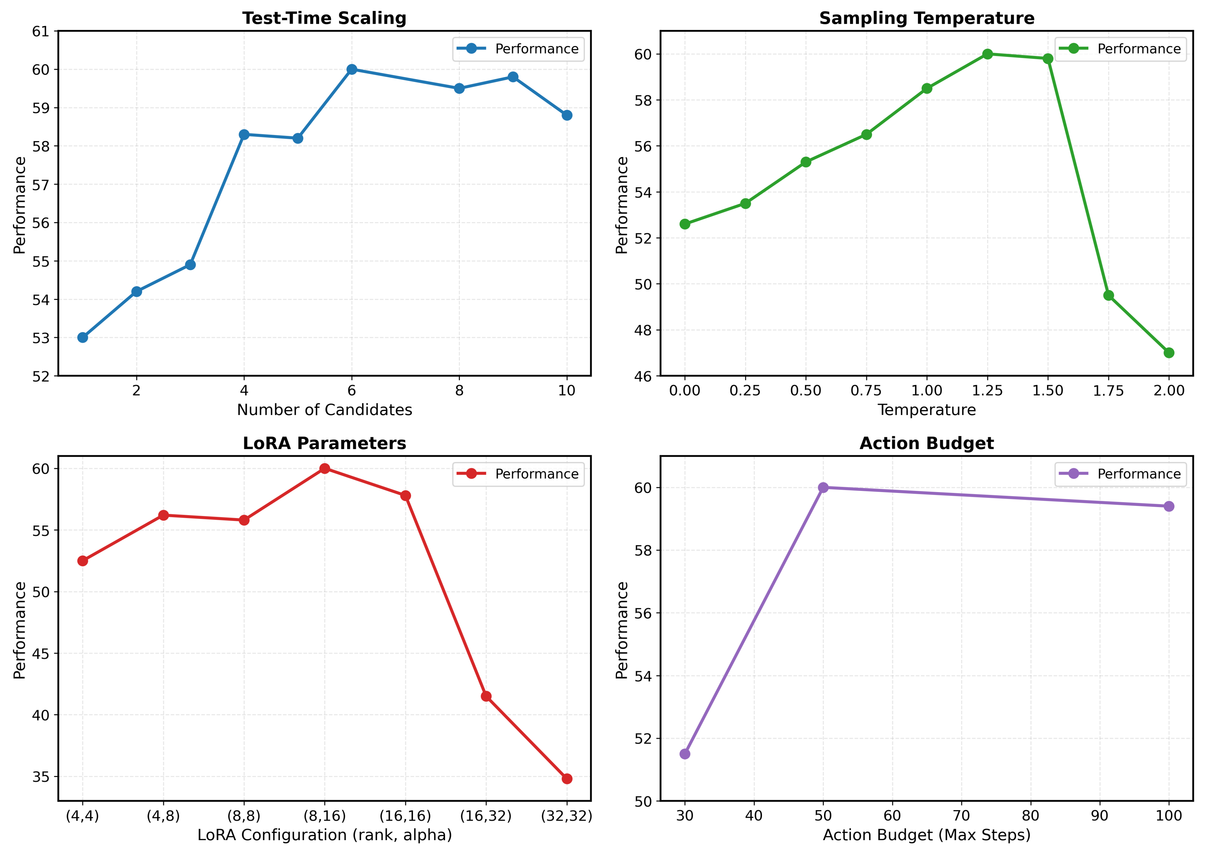
Figure 6 varies candidate count, temperature, LoRA capacity and action budget for cupboard fitting. It reports selected-point performance without error bars; causal explanations of small changes are hypotheses rather than isolated mechanisms.
N.1 Test-Time Scaling: Number of Candidate Actions
Fit performance rises from 53.0% at one candidate to 60.0% at six, then reaches 58.8% at ten. The curve is not strictly monotonic: N=4 slightly exceeds N=5. Six is the best tested point, not a universal optimal search width.
N.2 Sampling Temperature Analysis
Temperature 1.25 gives 60.0%, versus 52.6% for greedy decoding, 59.8% at 1.5, 49.5% at 1.75 and 47.0% at 2.0. Moderate diversity helps this scorer; high-temperature degradation is consistent with poorer candidate quality, but candidate-quality measurements are not supplied.
N.3 LoRA Configuration Analysis
The tested optimum is rank 8/alpha 16, 60.0% fit. Rank 4/alpha 4 gives 52.5%; rank 16/alpha 32 gives 41.5%; rank 32/alpha 32 gives 34.8%. The authors attribute large-adapter failure to repetitive outputs under aggressive updates on about 10–15 hindsight examples. Both rank and alpha vary, and the general method includes regularization despite this paragraph saying test-time training lacks it.
N.4 Action Budget Analysis
Increasing the maximum budget from 30 to 50 actions raises fit rate 51.5→60.0%; 100 actions gives 59.4%. No uncertainty is provided for the 0.6-point decrease, so accumulated-error explanations should not be treated as demonstrated causal effects.
Appendix O Single-Step Action Generation vs. Receding Horizon Planning
Compare single-action selection with generating 5–10 actions, executing only the first, updating, and replanning. Table 18 reports single-step fit/correct of 60.2/25.3% versus 57.8/25.8% for receding horizon, at relative compute 1× versus 5×. The latter slightly improves correct placement despite lower fit.
The prose alternates between 60.0 and 60.2% and between four-times-more and 5× compute; the table is retained as printed. This limited comparison does not establish a fundamental incompatibility between online training and receding-horizon planning. Hindsight can teach long-term consequences without explicitly regenerating a full plan each step.
| Method | Fit | Correct | Compute |
|---|---|---|---|
| Ours (Receding Horizon) | 57.8% | 25.8% | 5.0× |
| Ours (Single-Step) | 60.2% | 25.3% | 1.0× |
Appendix P Experiments on Long-Horizon Household Tasks: More Details
The household appendix details generation, physics filtering, observations, training and evaluation. Several reporting gaps remain: absolute SFT dataset size, full evaluation counts, human-rating sample sizes and hardware timings are not supplied in these descriptions.
P.1 Task Generation & Validation Overview
Initialize scenes, place generated objects, execute trajectories and capture observations after each interaction. Compare execution outcomes with the generated task specification before retaining examples; this supplies supervised action/reflection tuples.
P.2 Why Build Upon BEHAVIOR?
BEHAVIOR provides scene assets, object affordances, simulation and interaction interfaces; the authors add tasks designed around failure recovery and delayed consequences. Its name denotes 1,000 activities, while this appendix’s claim of “1,000+ scenes” is not established by the paper’s experiment inventory.
P.3 Task Categories
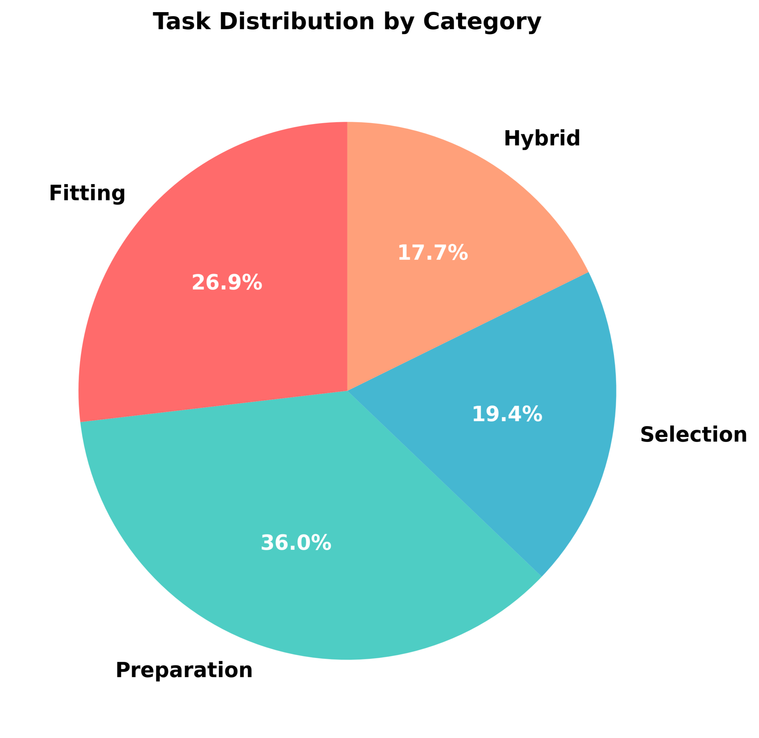
Fitting introduces size, occlusion and blocked-capacity failures; Selection rewards exploring for better alternatives; Preparation enforces prerequisite order; Hybrid combines these dependencies. Figure 7 gives category proportions of 26.9/19.4/36.0/17.7%, which should not be confused with the equal-category averaging in Table 1.
P.4 GPT-5 Task Generation Prompting Strategy
Prompts include room connections, object boxes/affordances, explicit failure modes and 2–3 examples per category. Required outputs interleave angle-bracket actions, internal critiques, execution status, external critiques and hindsight updates. Low-score unexecuted actions train the internal evaluator, not the action policy.
Calibration bands are 0–20 physical failure/dead end, 21–40 strategically harmful, 41–60 acceptable/suboptimal, 61–80 good and 81–100 near-optimal. Prompt refinement adds geometry and diverse failure examples. The paper describes this recipe but does not print a complete reusable generation prompt.
P.5 Physical Validation in BEHAVIOR.
Reject impossible placements and any trajectory whose annotated success/failure disagrees with simulation. Use uniform object scaling. Three external 560×560 RGB-D views are transformed into robot-base-frame point clouds after interactions; retain the most recent room observation. Validation is relative to this simulator and labeling procedure.
P.6 Training Data Construction
Four exact input/output schemas are retained below. Action inputs contain task/rooms/observations and previous feedback; internal scoring adds a proposed action; external scoring adds executed action, outcome and before/after observations; hindsight adds the historical action, room history and last reflection. The printed schemas have minor brace inconsistencies, preserved without silent correction.
Equations
| Input: | |||
| Output: |
| Input: | |||
| Output: |
| Input: | |||
| Output: |
| Input: | |||
| Output: |
P.7 Model Architecture and Training
Household models use a 3D encoder, multimodal projector and Llama-based 7B backbone. Unified SFT uses AdamW, learning rate 2×10⁻⁵, per-GPU batch eight, four-step accumulation, three epochs and weight decay 0.01. Fused point-cloud memory follows 3DLLM-Mem. Three copies are then instantiated, with only the external evaluator frozen.
This three-epoch configuration is not reconciled with Table 2’s peak at 100% data/one epoch. Keep the reported configuration and sensitivity result distinct.
P.8 Test-Time Training Configuration
Household LoRA uses rank four, alpha eight, dropout 0.15 on query/value projections. Internal-reflection updates use rate 5×10⁻⁵, three epochs and gradient clipping 0.3; action updates use SGD at 10⁻³, three epochs and clipping 0.5. Mix equal hindsight and self-distillation examples. These settings differ from cupboard LoRA.
P.9 Evaluation Protocol and Baselines
Require all task constraints within 30 actions; trigger hindsight at room exits or K=5 steps. Main deployment uses model-generated reflections grounded in simulator outcomes; the human-oracle study is a separate intervention.
Baselines include contextual reflection, up to three Self-Refine rounds, learned value scoring, spatial memory, PPO and Dreamer-style world-model learning. Matching environment-interaction counts is not necessarily matching computation. The appendix labels a DreamerV3 citation with the RoboDreamer reference, a bibliographic mismatch retained in the original references.
Appendix Q Cupboard Fitting: More Details
Cupboard experiments isolate placement failure with images and structured high-level commands rather than household point-cloud navigation.
Q.1 Cupboard Setup
Each task has 6–8 compartments and 6–10 objects. Compartments have known bounding boxes; multiple objects can share space. The authors stipulate one valid complete designated arrangement. Reported rates are fractions of placed objects, not the fraction of episodes that realize this complete solution.
Q.2 Base Model and Supervised Fine-tuning.
Use Qwen2.5-VL-3B with unified action/internal/external SFT: global batch 128, AdamW, learning rate 10⁻⁵, weight decay 0.1 and three epochs. This is the explicit 3B configuration, distinct from the household 7B description.
Q.3 Test-Time Training Variants.
Base-weight adaptation freezes vision and updates nonvisual parameters with SGD for three epochs: 10⁻³ for actions, 5×10⁻⁵ for the internal evaluator, weight decay 10⁻⁴ and no momentum. LoRA targets linear layers outside vision, embeddings and output head, with rank eight, alpha 16 and dropout 0.1; learning rates are 10⁻² for actions and 0.2 for the evaluator. Reported trainable-parameter reduction exceeds 95%, but the paper gives no full memory/latency accounting.
Appendix R More Qualitative Examples
The full Figure 8 preserves the gift-box search and both cupboard sequences. Local feedback first revises failed placements; later hindsight downgrades a previously acceptable box or watermelon placement after better choices or blocked capacity become visible. These are selected, simplified traces, not quantitative evidence of how often each behavior occurs.