Overview
This edition covers the ICLR 2026 paper, arXiv v1 dated 24 February 2026, including all six appendices. Antoine Bergerault completed the work while visiting UC Berkeley as an EPFL master’s student and is now at the University of Zurich. The original formal statements and equations are retained alongside concise explanations; notation and proof qualifications are identified where they affect interpretation.
At a glance
Matching a Nash expert’s demonstrated behavior need not yield a policy robust to another player’s strategic deviation. State-only matching can fail despite full state coverage; even state–action matching can fail when demonstrations miss states reachable after a deviation.
The paper states a PPAD-hardness result for a tight best-case exploitability bound, then derives upper bounds under strategic dominance or a stronger best-response sensitivity condition. A small regularized tag game illustrates the latter. These are conditional theoretical results, not an offline learning algorithm or broad empirical guarantee.
1 Introduction
ValueGap compares each player’s return with the expert’s return; NashGap measures the largest gain available from a unilateral deviation. Good joint imitation can satisfy the first criterion while remaining exploitable under the second.
A consistent bound vanishes with imitation error, and a tractable bound is computable efficiently from its assumptions. Exact matching is first analyzed, then approximate matching and game-dependent sensitivity. Zero Nash gap means a Nash equilibrium, which may be mixed; the introduction’s reference to a pure equilibrium is stronger than its definitions warrant.
2 Previous work
The background connects single-agent imitation guarantees with multi-agent strategic failures and prior coverage/concentrability assumptions.
Single-agent Imitation Learning.
Behavioral cloning fits expert actions, inverse reinforcement learning fits rewards, and GAIL matches occupancy measures adversarially. Single-agent analyses bound return loss from imitation error; they do not directly measure how another strategic player can exploit a learned policy.
Multi-agent Imitation Learning.
Multi-agent extensions support driving, crowds and robot interaction, but reward ambiguity and strategic deviations complicate their interpretation. Independent cloning produces product policies; matching jointly generated demonstrations alone does not certify Nash behavior.
Theoretical Barriers for MA-IL.
Tang et al. distinguish value from regret; Freihaut et al. provide bounds involving a deviation-related concentrability coefficient. Such coefficients may be unbounded or hard to compute. This paper instead seeks conditions on support and best-response changes.
3 Preliminaries
The model uses discounted Markov games, independent stochastic policies and normalized occupancy measures. The exact definitions of equilibrium, value loss, exploitability and imitation error are preserved below.
3.1 Markov Games
n players act simultaneously with product policy π₁×⋯×πₙ, rewards in [−1,1], initial distribution ν₀ and discount γ<1. State occupancy is the normalized discounted visitation distribution; state–action occupancy multiplies it by the joint policy.
The displayed state-value formula uses occupancy defined from ν₀, so its right-hand side does not depend on the displayed state s. Read it as the ν₀-averaged value unless occupancy is reinitialized at s; the printed formula is preserved unchanged.
Equations
3.2 Measuring optimality in games
A best response maximizes a player’s discounted return against fixed opponents. A Nash equilibrium is a product policy in which every component is a best response. Policies may be stochastic; independent does not mean deterministic, and a correlated joint policy is outside this definition.
Equations
Definition 1 (Best-response mapping).
For an agent , the best-response mapping to is defined as
Definition 2 (Nash equilibrium).
A policy is a Nash equilibrium of the game if is a product policy and each individual policy is a best-response to the other policies, i.e.
3.3 Offline Imitation learning
Offline data consist of expert-equilibrium trajectories, without further environment access. NashGap is the maximum unilateral improvement, while ValueGap is the largest expert-minus-learner return difference. Rewards imply the trivial exploitability bound 2/(1−γ).
BC error is the maximum per-player L1 policy error averaged under expert state occupancy. State and state–action errors are L1 distances between true occupancy measures. These are population quantities; an empirical training loss does not certify them without additional estimation/generalization arguments. Known value-loss bounds need not transfer to NashGap.
Equations 1–2
Definition 3 (Value gap).
Given an expert policy of , the Value gap of a policy is:
Definition 4 (Nash gap, see Ramponi et al. (2023)).
We define the Nash (imitation) gap of a product policy of the game as
| (1) |
with any .
| (2) |
4 Impossibility results for exact measure matching
Exact state–action matching identifies the expert only where expert occupancy is positive. Full-state support closes that gap; removing support coverage or discarding action information permits horizon-sized exploitability. The counterexamples establish failure in general games, not failure of every incomplete-coverage task.
Equation
4.1 Sufficiency of state-action matching under full-state support
Summing equal state–action measures over actions gives equal state occupancies. Dividing by a positive occupancy then recovers the same action distribution at that state. With full support, the entire policy equals the expert and therefore has zero Nash gap.
This is an exact population statement. Full support alone supplies neither a useful finite-sample guarantee nor a lower bound on how often rare states appear.
Equations
Theorem 1.
Let be such that . Then, and for every .
Corollary 1.
Let be such that and ; then, .
4.2 Insufficiency of state-only matching with full-state support
The three-state cooperative example uses a uniform initial distribution, so every state has positive occupancy. The expert repeatedly takes the rewarding cycle, while another joint policy self-loops with reward −1 and the same uniform state occupancy.
One player can restore the expert cycle by deviating, gaining 5/[3(1−γ)]. Thus matching visited-state frequencies loses strategically important action information, even when coverage is complete. Both transition and reward diagrams remain.
Equation
Lemma 1.
There exists a game and a corresponding expert policy such that . Moreover, there exists a policy such that and .
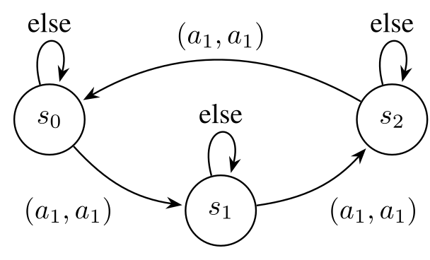
Diagram mathematical labels
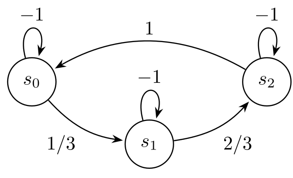
Diagram mathematical labels
Equations
4.3 Insufficiency of state-action measure matching with unvisited states
An imitation policy can agree with the expert on every observed state–action pair yet behave differently at an unvisited state. A unilateral deviation can reach that state and exploit the difference. Theorem 2, adapted from Tang et al., gives an order-1/(1−γ) gap; Appendix B.3 supplies the explicit construction.
Equation
Theorem 2.
(Adapted from Tang et al. (2024, Theorem 4.3)) There exists a Markov Game with expert policy and a learned policy such that even if , the Nash gap scales linearly with the discounted horizon; i.e., .
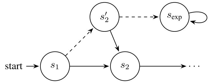
We can design reward functions for the transitions of Figure 2 such that the expert would always take the solid arrows.
The dataset missing information about , a best-response can lead to states then . This last state can be designed to incur high rewards for one player, while the expert region incurs linear less.
Diagram mathematical labels
5 On the Infeasibility of Tractable Lower Bounds for Exploitability
The tight lower bound minimizes NashGap over both expert equilibria and learned policies at exactly a prescribed state–action distance. It is a best-case quantity over a constrained family, not the exploitability of one supplied policy or a worst-case learning guarantee.
Theorem 3 states that computing this quantity is PPAD-hard even for known bimatrix games, with a Markov-game corollary. This does not forbid loose bounds or special tractable games, nor does PPAD-hardness prove that no polynomial algorithm can exist.
The reduction is retained in full mathematical form. Its support-recovery argument has unresolved details: the displayed linear programs omit comparisons against actions outside the supplied support, and the approximate-support argument does not specify the required approximation regime. These limit what can be inferred directly from the printed proof.
Equations
Definition 5 (Tight Nash gap lower bound).
Let be a Markov Game and let the set of Nash equilibria of . We define the tight Nash gap lower bound for with occupancy matching error as
where .
Theorem 3.
Corollary 2.
The problem of computing given an arbitrary Markov game and an arbitrary is PPAD-hard.
6 Tractable and Consistent Exploitability Upper Bounds from Best-Response Continuity
The positive results separate ordinary imitation error from how much optimal responses can change when opponents depart from equilibrium. The resulting upper bound is useful only when that game-dependent sensitivity can itself be controlled and estimated.
6.1 Characterization of Markov Games via Best-Response delta-continuity
Definition 6 bounds the distance from the expert to every best response after a small change in the opponents’ joint policy, measured on expert-visited states. This is stronger than continuity of one selected response: ties can already make the maximum large.
A long chain makes a strategically decisive state rare in discounted occupancy, so a small BC error can switch a best response across the visited region. This defeats any uniform nontrivial δ over the broad class considered. The example’s additional claim that zero state-only error is equivalent to zero BC error is not justified: player-2 actions affect rewards while leaving its state transitions unchanged.
Equations
Definition 6 (-continuity of the best-response correspondence).
For a given game , the best-response mapping is said to be -continuous at equilibrium for some if for all , and , we have:
Definition 7 (-continuity of a class of games).
A class of Markov Games is -continuous if every game is -continuous at all its Nash equilibria.
Lemma 2.
Let be the class of games with consistent bounds. This class is -continuous only for trivial such that for all .
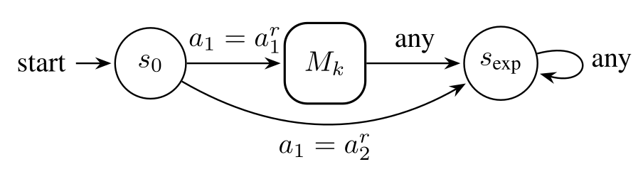
Diagram mathematical labels
Equations
6.2 Provable convergence under strategic dominance
At a weak dominant-strategy equilibrium, each expert component remains a best response against any opponents. Adding/subtracting the expert value and bounding two policy differences gives NashGap ≤2nϵBC/(1−γ)²; the appendix obtains the slightly sharper coefficient 2n−1. The corollary inverts this bound to select a sufficient BC tolerance.
Weak dominance permits other tied best responses far from the expert. It therefore suffices for this value argument but does not imply δ=0 under Definition 6’s maximum over all best responses, despite the source’s stated equivalence.
Equations 3
Definition 8 (Dominant Strategy Equilibrium (DSE)).
A policy is a (weak) dominant strategy equilibrium if for every player , is a weak dominant strategy, i.e.:
Lemma 3.
Suppose is a (weak) Dominant Strategy Equilibrium. Then, any learned policy with BC error satisfies .
| (3) |
Corollary 3.
Suppose is a (weak) Dominant Strategy Equilibrium; then, the recovered behavioral cloning policy is an -Nash equilibrium if .
6.3 Relaxing the dominance assumption
Lemma 4 prints NashGap ≤[2nϵBC+δ(ϵBC)]/(1−γ)². Its proof adds the distance between the new best response and the expert to the ordinary imitation terms.
For more than two players, Definition 6 measures the opponents’ joint-policy error, whereas ϵBC is per player. The product-distribution bound gives joint error at most (n−1)ϵBC. Substituting δ(ϵBC) therefore needs an additional interpretation or stronger assumption; the source does not supply it. The numerical experiments are two-player.
Equation
Lemma 4.
Suppose the equilibrium expert is and the game is -continuous at . Then, .
Properties of the bound.
An efficiently computable valid δ makes the displayed bound computable. A bound that vanishes as error tends to zero requires δ to tend to zero there, not merely an isolated declaration δ(0)=0. Computing a valid δ for an arbitrary game is not solved by expressing the bound in terms of it.
On the sensitivity of game equilibria.
Best-response sensitivity can remain informative where deviation occupancy has poor overlap with demonstrations. Conversely, the trivial δ=2 makes the proposed bound looser than the basic reward-range bound.
Entropy regularization may smooth responses, and risk aversion is proposed as another direction. These modifications change the optimization/game being studied. The paper does not prove that increasing regularization always reduces the unregularized game’s exploitability.
7 Conclusion
The practical message is to evaluate strategic robustness separately from imitation fit. Coverage, unilateral deviations and response stability determine whether an imitation error is meaningful for equilibrium learning. Reachability assumptions, stronger distribution control and demonstrations of off-equilibrium behavior are proposed future directions.
Acknowledgments
Support came from NSF grants ECCS-2438314 and CCF-2423134, Army Research Laboratory grant W911NF-26-1-0002 and EPFL.
Appendix A Additional background
The background appendix defines the complexity class used in the hardness claim and explains the occupancy-matching view of adversarial imitation.
A.1 PPAD complexity class
PPAD is defined through polynomial reduction to End-of-the-Line: from one source in an implicitly represented directed graph with at most one predecessor/successor per vertex, find another source or a sink. The parity argument guarantees a solution, placing these search problems within TFNP.
General Nash computation is the motivating example. PPAD-hard is a conditional computational barrier, not an unconditional impossibility result. The original problem definition and references are retained.
Equation
Definition 9 (PPAD class).
A search problem belongs to the complexity class PPAD (Polynomial Parity Arguments on Directed graphs) if and only if it is polynomial-time reducible to the End-of-the-Line problem defined as follows:
End-of-the-Line Problem
Input:
- •
A directed graph implicitly represented by two polynomial-time computation mutually inverse functions and :
- –
maps every vertex to its unique predecessor, or itself.
- –
maps every vertex to its unique successor, or itself.
- •
A source vertex such that and .
Output: Either a sink vertex or another source vertex.
A.2 GAIL and occupancy-measure matching
GAIL combines cost inference and entropy-regularized control into a discriminator/policy minimax objective. With the stated regularizer and unrestricted cost class, it corresponds to Jensen–Shannon state–action occupancy matching plus an entropy term.
This connection explains the matching errors analyzed in the paper. It does not turn occupancy agreement into a strategic guarantee, and the occupancy objective should not be conflated with supervised BC.
Equations
Appendix B Proofs of hardness results
The hardness appendix proves policy identification on visited states, supplies explicit failure games, and presents the support-based reduction claimed for the tight lower bound. All proof equations and the reduction algorithm are preserved.
B.1 Proof of Theorem 1
Equal state–action occupancies force the same visited region: a positive action probability at a visited state would otherwise contradict equality. Within that region, their action marginals agree and normalized conditional policies must coincide. Nothing constrains behavior where both occupancies vanish.
Equations
B.2 Proof of Nash equilibria for the game in Figure 1
Against an opponent always taking a₁, a unilateral a₂ produces the worst reward and a self-loop. Its advantage cannot be positive when the expert value is at least −1/(1−γ), establishing the cycle policy as a Nash equilibrium. The original advantage algebra is retained.
Equations
B.3 Proof of Theorem 2
In the infinite chain, odd states reward one and even states reward zero. Expert and learner follow the same even branch, but differ at the unvisited first odd state. A deviating player can exploit the learner there and continue through rewarding states; the expert’s off-path response prevents that gain.
The printed lower bound is 1/(1−γ)−1. The explicit policy and all transitions are retained; the example explains why identical demonstrated occupancy does not identify strategic off-path behavior.
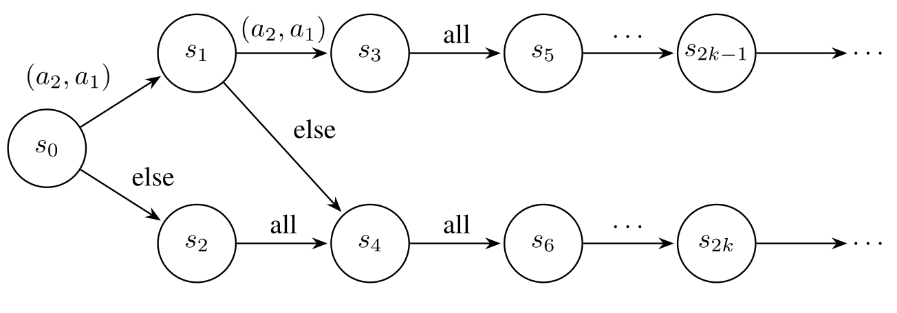
Diagram mathematical labels
Equations
B.4 Proof of Theorem 3
The claimed reduction first seeks an approximate equilibrium support, then uses a tight-lower-bound oracle to identify it. Exact support recovery and approximate support recovery are distinct subclaims, each with its original statement retained.
Equation
Lemma 5.
Finding an -Nash equilibrium support in a general bimatrix game is PPAD-complete.
B.4.1 Proof of Lemma 5
For an exact known equilibrium support, indifference equalities and probability normalization motivate a linear feasibility problem. The printed program includes only equalities among supported actions; it omits inequalities ruling out profitable unsupported actions. A feasible solution to the displayed constraints alone need not be an equilibrium.
The approximate version replaces indifference equalities with ±ϵ slack. Approximate Nash regret does not require every supported action to be within ϵ of every other supported action: a poor action can have tiny probability. The displayed argument therefore needs additional support/approximation conditions; the programs remain unchanged for inspection.
Equations
Theorem 4.
Finding the support of any Nash equilibrium in a bimatrix game is PPAD-complete.
B.4.2 Reduction for the proof of Theorem 3
Algorithm 1 depresses candidate action payoffs to a value K below the original rewards and queries the lower-bound oracle. Its comparison with a baseline s decides whether to retain each action, aiming to recover a lexicographically selected support with polynomially many calls.
The argument assumes that a change in the constrained minimum identifies an indispensable support action. Its oracle-error notation switches between δ and s in the minimizer definition, and the support-selection step is asserted rather than fully established by the displayed constraints. These are qualifications on the printed reduction, not alterations to its formal statement.
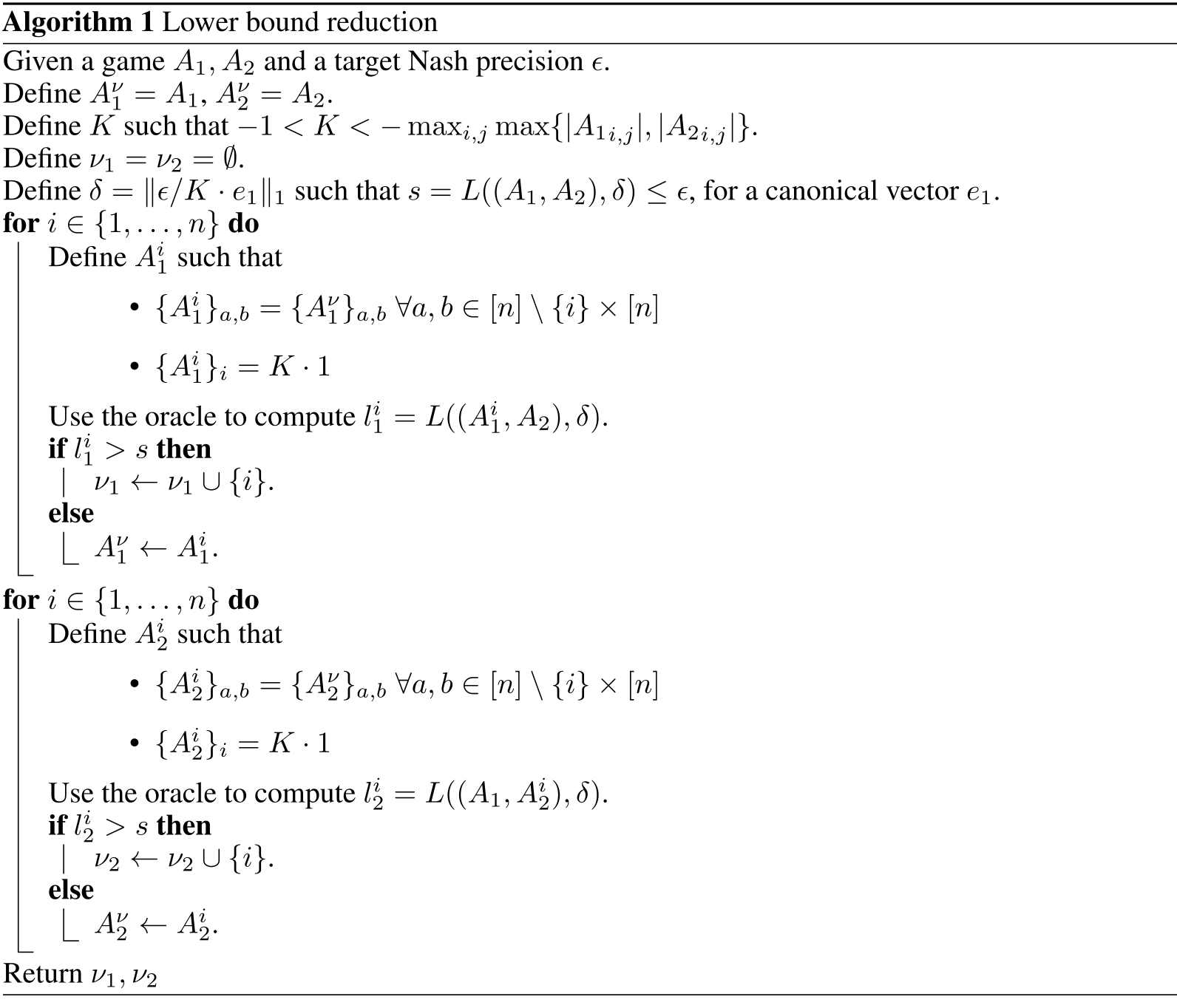
Copyable reduction algorithm
Given a game and a target Nash precision .
Define , .
Define such that .
Define .
Define such that , for a canonical vector .
for do
- •
- •
if then
- •
- •
if then
Equations
Appendix C Proofs of upper bounds
The upper-bound proofs use performance differences, bounded rewards and the L1 distance between product policies. Their dependence on the best-response assumption is explicit.
C.1 Proof of Lemma 3
Dominance allows replacing the optimizing deviation by the expert’s own component. Insert the all-expert value between learner and mixed-profile values; bound both differences under expert occupancy by the supremum Q-value and policy L1 error.
The product bound contributes n errors for the joint policy and n−1 for opponents, yielding (2n−1)ϵBC/(1−γ)². This reasoning is applied per player before maximizing; a displayed intermediate subtraction of two maxima should not be read as a generally valid identity.
Equations
C.2 Proof of Lemma 4
Without dominance, insert the actual best response. Triangle inequality separates opponent imitation error from response-to-expert distance, adding the δ term. The same product-policy accounting gives 2n−1 for ordinary errors. The joint-versus-per-player δ argument qualification from Section 6.3 still applies.
Equations
Appendix D Additional lemmas
Lemma D.1 expresses return differences as an advantage expectation under the alternative policy’s occupancy. Lemma D.2 proves that the L1 distance between product distributions is at most the sum of component L1 distances.
For the product lemma, add/subtract one mixed product, apply triangle inequality and use probability normalization; induction extends the two-factor step. These identities explain both the horizon factors and the linear dependence on the number of players.
Equations
Lemma D.1 (Performance Difference Lemma, see e.g. Theorem IX.5 in Alatur et al. (2024)).
For any ,
where .
And more generally,
Lemma D.2.
Let , and let be probability distributions over a discrete set of size isomorphic to . Further, note . Then,
Appendix E Numerical Validation
The numerical example is a two-player zero-sum tag game on a 2×3 grid with γ=0.8. Players move in four directions, exchange tagger roles on contact and receive boundary penalties. Two nonsymmetric corner initializations represent the tested starts.
A regularized Nash value-iteration solution supplies the expert. Random perturbations generate imitation policies; 2,000 episodes estimate expert occupancy, and induced-MDP value iteration computes responses. The resulting cumulative maxima are estimates over sampled policies, not certified uniform envelopes over all deviations.
Equation
E.1 On the validity of the upper bound (Lemma 4 )
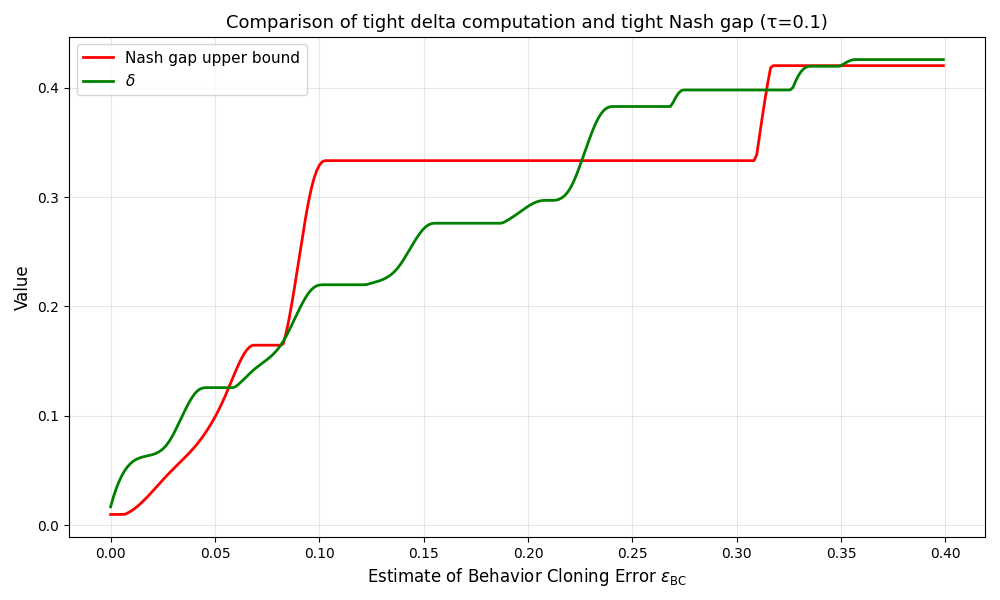
With temperature 0.1, 400 noise levels span [0,0.4]. The plot compares sampled cumulative maxima of Nash gap and response distance; both generally increase with BC error. The proposed horizon-squared bound is loose in this toy game.
Agreement with these samples illustrates the conditional theory but cannot independently prove a valid global δ or the bound for arbitrary games. The plot’s “tight” terminology refers to the sampled envelope.
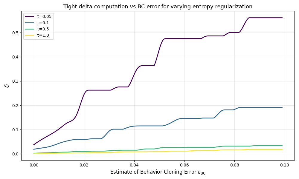
E.2 On the impact of entropy regularization
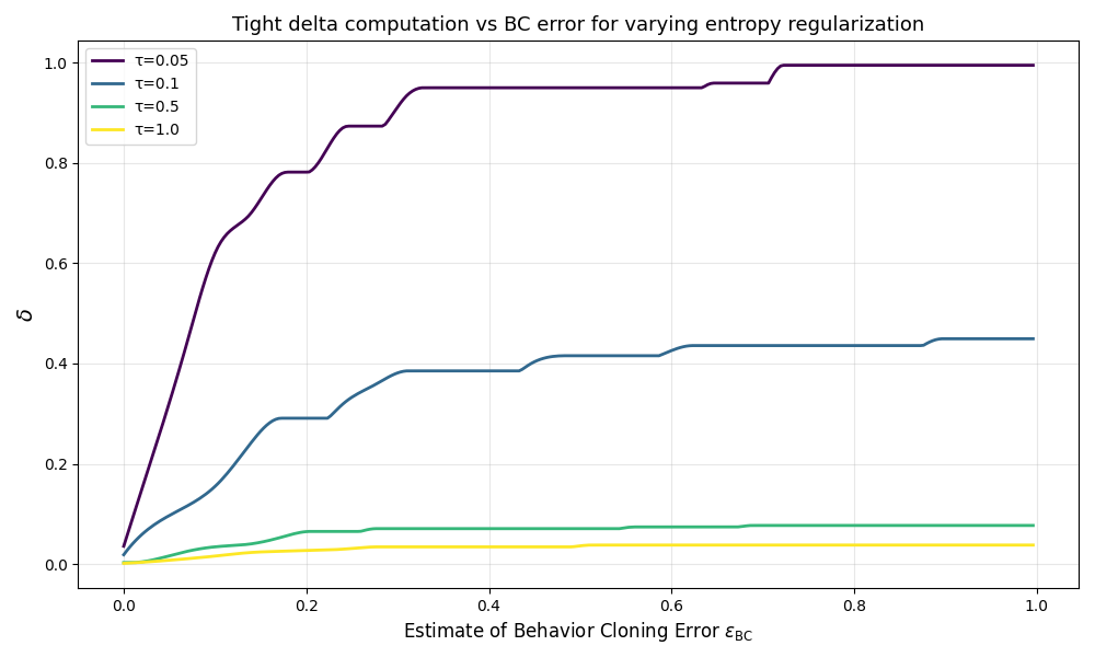
Using 250 perturbations across noise levels [0,1], higher entropy temperatures reduce the estimated response-sensitivity envelope in this game. The same trend is shown near BC error 10⁻².
Lower δ does not necessarily lower actual NashGap because the bound is not tight and regularization changes the equilibrium/response objective. The paper explicitly limits this inference; extensions to human demonstrations and risk aversion remain motivation rather than established results.
Appendix F Finite horizon case
The finite-horizon appendix replaces discounted occupancy with time-indexed visitation and develops analogous counterexamples and H² upper bounds. The full finite-horizon formulas are preserved, including notation irregularities.
F.1 Definitions
Policies and rewards become time-dependent over H stages. Error assumptions take a maximum over time, which differs from an average under discounted occupancy.
F.1.1 Finite horizon Markov Games
Each time t has a state distribution μᵗ and state–action distribution ρᵗ. Values accumulate rewards from t through H−1. The printed value definition keeps t in its summand while summing over h, and omits explicit conditioning on the starting state; those indexing/conditioning details require interpretation.
Equations
F.1.2 Assumptions on matching errors
Finite-horizon BC error is the largest expert-occupancy-averaged per-player L1 error over all times. State-only and state–action errors likewise take the maximum time-indexed occupancy discrepancy. These worst-time quantities should not be replaced by average training error.
Equation
F.2 Performance difference lemma for finite horizon
Expand the Q-function one step, add/subtract the reference value, and telescope through the H stages. This yields a sum of reference-policy advantages evaluated under the alternative trajectory distribution. The more general joint-policy statement follows the same construction; the source’s malformed closing-parenthesis notation remains visible.
Equations
Lemma F.1 (Finite horizon version of Lemma D.1).
For any ,
where .
And more generally,

Original source MathML
F.3 Results
The appendix states finite analogues of the matching impossibilities and response-sensitive bounds. It preserves the same distinction between lack of action information, missing coverage and unstable best responses.
F.3.1 Section 4
The three-state example gives order-H exploitability despite state-only matching. Truncating the off-path chain yields a finite-state, finite-horizon example with matching state–action distributions at each time but order-H exploitability.
Equations
Lemma F.2 (Finite version of Lemma 1).
There exists a game and a corresponding expert policy such that . Moreover, there exists a policy such that and .
Theorem F.1 (Finite horizon version of Theorem 2).
There exists a Markov Game with expert policy and a learner policy such that even if for all , the Nash gap scales linearly with the horizon; i.e., .
F.3.2 Section 6
Dominance gives NashGap ≤2nϵBC H² by bounding each stage’s Q-values by H and summing H occupancy-weighted errors. A response-distance assumption adds δ(ϵBC)H²; the appendix again obtains the sharper 2n−1 coefficient before relaxing it.
The claimed finite-horizon sensitivity counterexample only says to adapt the chain length k. It does not spell out how discounted rarity becomes small occupancy under the newly defined worst-time errors. Lemma F.5 also states an order-δ assumption but prints a unit-coefficient δ bound; any hidden constant needs to be retained when applying it.
Equations
Lemma F.3 (Finite horizon version of Lemma 2).
Let be the class of games with consistent bounds. This class is -continuous only for trivial such that for all .
Lemma F.4 (Finite horizon version of Lemma 3).
Suppose is a (weak) Dominant Strategy Equilibrium. Then, any learned policy with BC error satisfies .
Lemma F.5 (Finite horizon version of Lemma 4).
Let be the learned policy, and assume for all and that for some function , where . Then, .