At a glance
FLAM learns a video world model with separate latent actions for scene factors rather than one action for the entire image. Jointly learned slot representations, inverse dynamics, and forward dynamics improve multi-entity reconstruction and prediction on four simulated datasets and driving video. Downstream experiments use a small action-labeled subset to decode latent actions and pseudo-label larger demonstrations. Prediction benchmarks infer latent actions from the true future video, so their scores measure reconstruction under inferred controls, not unconstrained forecasting from an initial image alone.
1 Introduction
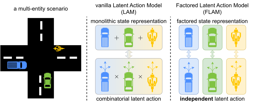
When several entities move independently, one scene-wide action must encode their combinations. FLAM assigns each learned factor its own action while sharing the dynamics networks and action prior across factors. This encourages reuse of individual motion patterns. Factors need not be individual visual objects: correlated entities can share a factor, and interactions remain possible through conditioning on the current scene’s slots.
2 Related Work
Observation-only methods such as LAPO and Genie infer a latent transition control and train a predictor conditioned on it. Factored decision models motivate splitting complex state/action spaces, while Slot Attention provides a learnable decomposition of image features.
FLAM jointly trains its factorizer and dynamics on future-feature prediction. This differs from freezing a separately learned object reconstruction representation before dynamics training, as in the compared object-centric baselines. Its intended grouping is driven by transition structure rather than visual appearance alone.
3 Preliminaries
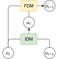
An inverse model sees current and next observations and infers a latent action; a forward model sees the current observation and that action and predicts the next observation. Restricting the action channel prevents the inverse model from simply copying the entire future. These latents capture useful transition information but need not coincide uniquely with real commands: visually indistinguishable outcomes can yield indistinguishable inferred actions.
4 Factored Latent Action Model (FLAM)
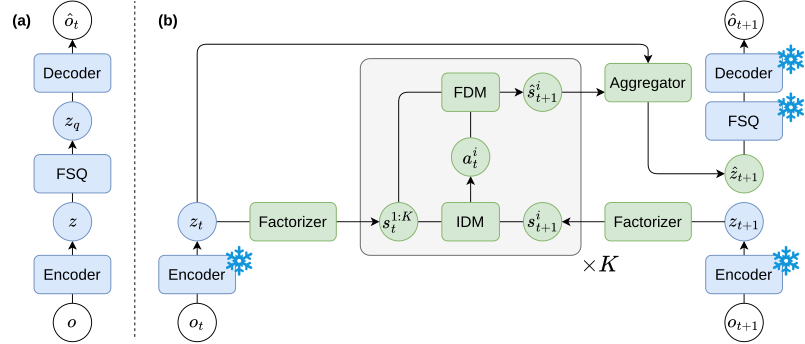
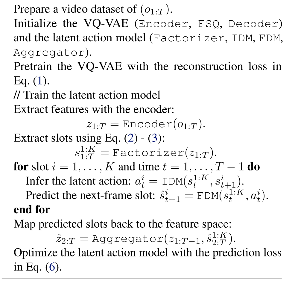
Training first learns a dataset-specific image tokenizer and decoder, then freezes them while learning factorized dynamics in feature space. The factorizer, inverse model, forward model, and feature aggregator train jointly in the second stage. Afterwards, inferred latents can steer generated sequences or support action pseudo-labeling for behavior cloning.
4.1 Pretrained Encoder
A convolutional encoder maps pixels to patch features, finite scalar quantization constrains their representation, and a decoder reconstructs the image. Reconstruction loss trains this tokenizer separately for each dataset. Subsequent world-model learning predicts its frozen features rather than raw pixels; decoder reconstruction quality therefore provides a useful reference for attainable visual fidelity.
Equations 1
| (1) |
4.2 Factored Latent Action Model (FLAM)
Slot Attention decomposes each frame’s features. Causal temporal attention lets each slot consult its own history, stabilizing its binding across time. For a particular factor, the shared inverse model reads all current slots plus that factor’s next slot and predicts a Gaussian latent-action posterior. A Kullback–Leibler penalty toward a unit-normal prior limits transition information.
The shared forward model predicts a factor’s next state from all current slots and that factor’s action. Thus action channels are separated while current-state interactions remain available. An aggregator attends from current image features to predicted slots, preserving static detail without forcing slots to reconstruct everything. Feature prediction error plus the summed posterior penalties trains all four modules. Shared weights make the same action space reusable; they do not establish statistical independence or physical identifiability of the learned factors.
Equations 2–4
| for | each slot attention iteration | |||
| (2) | ||||
| (3) |
| (4) |
Equations 5–6
| (5) |
| (6) |
4.3 Learned Latent Actions Utilization
For generation, a user selects an entity and substitutes sampled or chosen latent controls while other entities retain their inferred original actions. For policy learning, a small action-labeled demonstration subset trains a decoder from inferred latents to real actions. The decoder then pseudo-labels a larger video-only set, and a behavior-cloning policy learns from those labels. The downstream policy therefore still uses action supervision for calibration.
Equation 7
| (7) |
5 Experiments
Experiments use MultiGrid, three Procgen games, and front-camera nuPlan video. Each dataset has its own pretrained encoder; compared methods share that encoder and, where applicable, component architectures. FLAM and PlaySlot divide total latent-action dimensionality across factors to match the scene-wide baselines’ total dimension. Ground-truth-action World Model is evaluated only in simulation. The study demonstrates dataset-specific models, not one universal pretrained world model.
5.1 World Model Accuracy
Ground-truth evaluation videos supply the inverse model’s latent controls, followed by ten autoregressive prediction steps. Across five datasets, FLAM averages 34.9 PSNR, 0.890 SSIM, 0.051 LPIPS, and 419.6 FVD. It is best or tied on most individual comparisons, although AdaWorld’s Bigfish FVD is slightly lower, 63.3 versus 63.6. On nuPlan, FLAM’s PSNR is 19.7 versus 18.1 for AdaWorld and 16.0 for Genie; frozen reconstruction reaches 21.7.
Beating the action-conditioned World Model does not imply that inferred controls are more informative than complete physical actions: Procgen supplies only the player action, while FLAM’s posterior can encode other entities’ realized future changes; MultiGrid’s action baseline uses a monolithic joint token. Generation examples show factor-specific edits with other inferred controls fixed. They establish controllability in the examples rather than unrestricted intervention validity in the real world.
| Dataset | Metric | FLAM (ours) | AdaWorld | Genie | World Model | PlaySlot | SlotFormer | Recon |
|---|---|---|---|---|---|---|---|---|
| Average | PSNR () | 34.9 | 24.7 | 28.1 | N/A | 29.1 | 19.9 | 37.1 |
| SSIM () | 0.890 | 0.862 | 0.859 | N/A | 0.847 | 0.814 | 0.909 | |
| LPIPS () | 0.051 | 0.096 | 0.091 | N/A | 0.120 | 0.223 | 0.035 | |
| FVD () | 419.6 | 749.5 | 717.5 | N/A | 858.0 | 1597.7 | 215.1 | |
| MultiGrid | PSNR () | 56.5 | 24.0 | 33.9 | 56.1 | 56.5 | 24.9 | 56.5 |
| SSIM () | 0.944 | 0.909 | 0.933 | 0.943 | 0.944 | 0.912 | 0.944 | |
| LPIPS () | 3e-4 | 0.08 | 0.014 | 6e-4 | 3e-4 | 0.056 | 3e-4 | |
| FVD () | 2.9 | 913.6 | 177.5 | 5.5 | 2.9 | 451.6 | 2.5 | |
| Bigfish | PSNR () | 30.8 | 30.3 | 28.5 | 23.9 | 26.0 | 19.6 | 34.4 |
| SSIM () | 0.983 | 0.982 | 0.974 | 0.949 | 0.962 | 0.934 | 0.992 | |
| LPIPS () | 0.011 | 0.012 | 0.021 | 0.049 | 0.038 | 0.221 | 0.004 | |
| FVD () | 63.6 | 63.3 | 106.5 | 168.9 | 227.4 | 1455 | 16.8 | |
| Leaper | PSNR () | 38.1 | 23.3 | 35.0 | 24.7 | 27.5 | 21.4 | 40.3 |
| SSIM () | 0.976 | 0.924 | 0.973 | 0.924 | 0.945 | 0.913 | 0.977 | |
| LPIPS () | 0.002 | 0.072 | 0.005 | 0.044 | 0.031 | 0.164 | 0.001 | |
| FVD () | 12.1 | 348.1 | 27.3 | 127.3 | 361.5 | 1151 | 6.27 | |
| Starpilot | PSNR () | 29.3 | 27.8 | 27.0 | 25.8 | 18.3 | 19.8 | 32.6 |
| SSIM () | 0.971 | 0.965 | 0.962 | 0.959 | 0.886 | 0.907 | 0.980 | |
| LPIPS () | 0.015 | 0.023 | 0.028 | 0.040 | 0.187 | 0.166 | 0.006 | |
| FVD () | 73.4 | 113.4 | 141.0 | 194.9 | 792.0 | 720.9 | 24.7 | |
| nuPlan | PSNR () | 19.7 | 18.1 | 16.0 | N/A | 17.2 | 14.0 | 21.7 |
| SSIM () | 0.577 | 0.529 | 0.453 | N/A | 0.498 | 0.405 | 0.650 | |
| LPIPS () | 0.229 | 0.292 | 0.389 | N/A | 0.344 | 0.508 | 0.163 | |
| FVD () | 1946 | 2309 | 3135 | N/A | 2906 | 4210 | 1025 |
5.2 FLAM State Representation
With four MultiGrid agents and three slots, two agents forced to take identical actions can share a factor. With four independently acting agents and four slots, FLAM’s adapted disentanglement/completeness/informativeness scores are 0.91/0.91/0.93, compared with PlaySlot’s 0.81/0.81/0.86. These scores use position probes with per-frame optimal matching, so they do not independently prove globally fixed semantic slot identity. Reducing slots to two lowers PSNR to 53.4; four, eight, and sixteen slots all reach 56.5 in this four-agent setting.
5.3 Latent Action Policy Learning
An expert supplies one million demonstration frames per environment. A decoder trained on one thousand or ten thousand labeled frames pseudo-labels the rest. With ten thousand labels, episodic returns rise from 3.6 to 8.8 in Bigfish and from 6.4 to 9.1 in Starpilot versus labeled-only cloning. With one thousand labels, gains are small and nonuniform: Bigfish rises from 1.0 to 1.8, but Starpilot falls from 1.9 to 1.8. Limited decoder accuracy can make extra pseudo-labels unhelpful.
5.4 Ablation Studies
Temporal attention is important for stable factor assignments: removing it reduces MultiGrid PSNR from 56.5 to 51.6 and informativeness from 0.93 to 0.20. Allowing every predicted slot to use every latent action largely preserves prediction quality but weakens disentanglement and position information. The KL sweep is stable from 10⁻⁵ through 10⁻³; at 10⁻², PSNR collapses to 24.9 and FVD rises to 479.9. Robustness therefore has a clear tested limit.
6 Conclusion
Factorwise latent controls and joint dynamics-driven representation learning improve the tested multi-entity video models. Remaining limitations include dataset-specific tokenizers, restricted decoder fidelity, and no universal model. Evaluation uses posterior actions inferred from future video, and quantitative tables do not provide run-to-run uncertainty. More expressive diffusion/flow decoders and shared pretrained tokenizers are proposed extensions; physical closed-loop robot or autonomous-driving control is not demonstrated.
Impact Statement
The impact statement describes the work as advancing machine learning and does not identify a specific societal consequence for additional discussion.
Acknowledgments
The acknowledgments list the participating University of Texas laboratories, public and industry research funding, and a disclosure that Peter Stone is compensated as Sony AI’s Chief Scientist. The authors state that the university reviewed the arrangement under its research-objectivity policy.
Appendix A Dataset Details
Unless otherwise specified, data is split 80/10/10 by frame count for training, validation, and test. Inputs are normalized to zero–one. The appendix does not fully specify scene-level separation for every video-model dataset; policy demonstrations receive a separate disjoint-level protocol.
MultiGrid (Simulation).
MultiGrid uses eight-by-eight worlds rendered at 128-by-128 pixels, with two to sixteen simultaneously moving agents. The default experiment has four agents and four factors.
Procgen (Simulation).
The three Procgen games disable rendered backgrounds and use 224-by-224 images. This simplifies visual variation compared with the original full-background game distribution.
nuPlan (Real-world).
nuPlan contributes real driving video from front-facing cameras, resized to 224-by-224 pixels. Sixteen factors represent vehicles, pedestrians, and other scene changes. This evaluates video modeling rather than a driving policy.
Appendix B Implementation Details
Simulation uses an IMPALA-style encoder/decoder and nuPlan uses MAGVIT-v2 components. Finite scalar quantizers have 1,024 and 16,384 codes, respectively. Patch-feature dimension is 128; attention width is 256 with eight heads and two simulation or three real-video layers. The default latent regularizer is 2×10⁻⁴. Both training phases use AdamW at 10⁻⁴ learning rate, with batches of sixty-four for the tokenizer and thirty-two for dynamics.
| Simulation | Real-world | |
| Encoder architecture | IMPALA | MAGVIT-v2 |
| Decoder architecture | IMPALA | MAGVIT-v2 |
| Image size | 128 (Multigrid), 224 (Procgen) | 224 |
| 128 | 128 | |
| Tokenizer quantizer | FSQ | FSQ |
| Tokenizer codebook size | 1024 | 16384 |
| Tokenizer codebook levels | [4,4,4,4,4] | [4,4,4,4,4,4,4] |
| Optimizer | AdamW | AdamW |
| Learning rate | 1e-4 | 1e-4 |
| Batch size | 64 | 64 |
| Attention model dimension | 256 | 256 |
| Number of attention heads | 8 | 8 |
| Number of attention layers | 2 | 3 |
| Number of factors | 4 (Multigrid), 16 (Procgen) | 16 |
| KL regularization coefficient | 2e-4 | 2e-4 |
| Optimizer | AdamW | AdamW |
| Learning rate | 1e-4 | 1e-4 |
| Batch size | 32 | 32 |
Computational Cost
Patch–slot attention scales as O(NK), and interactions among K slots as O(K²) per timestep, versus O(N²) for dense patch attention. This comparison explains a potential saving when slots are much fewer than patches; it is not a measured end-to-end runtime, memory, or scaling-law guarantee.
Appendix C Experiments
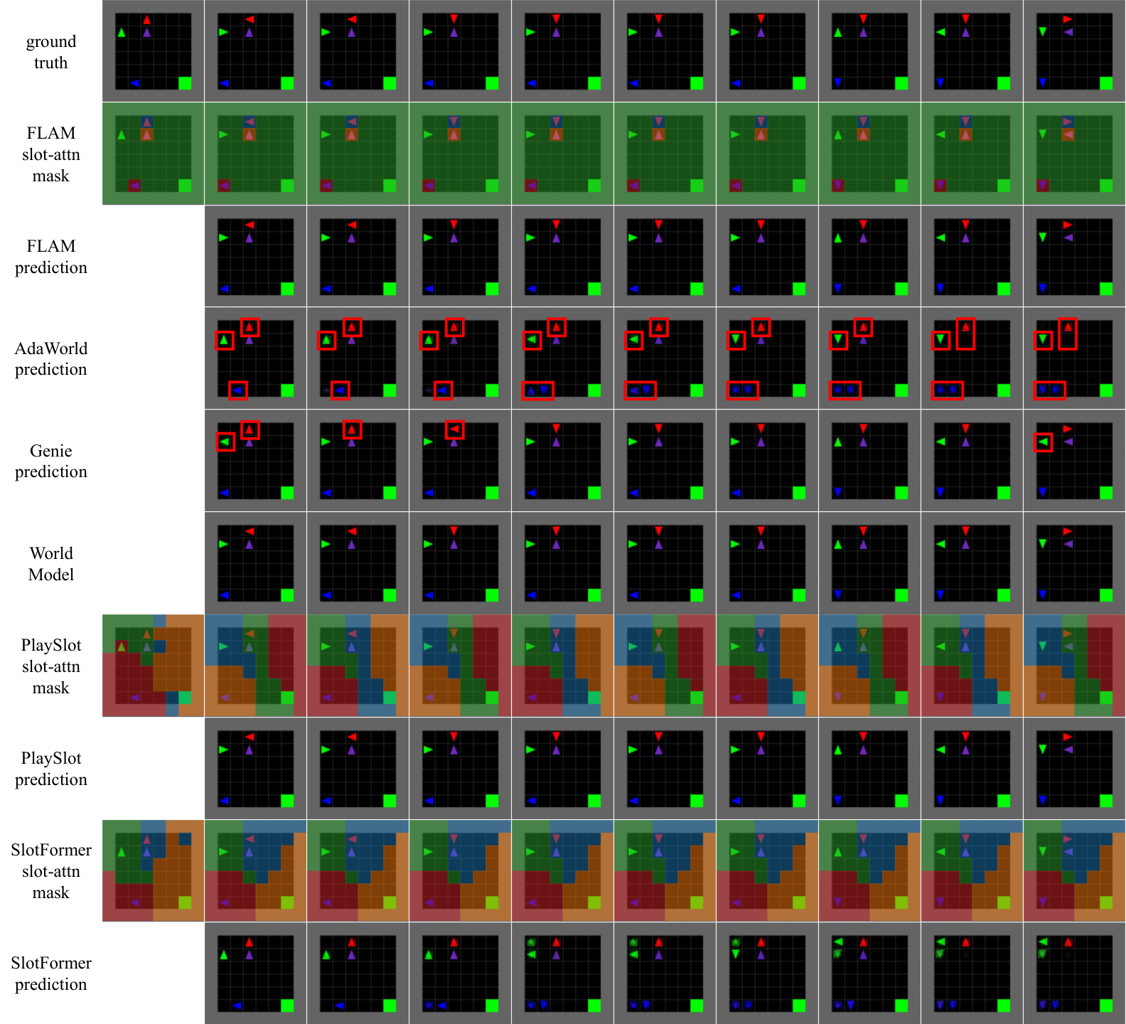
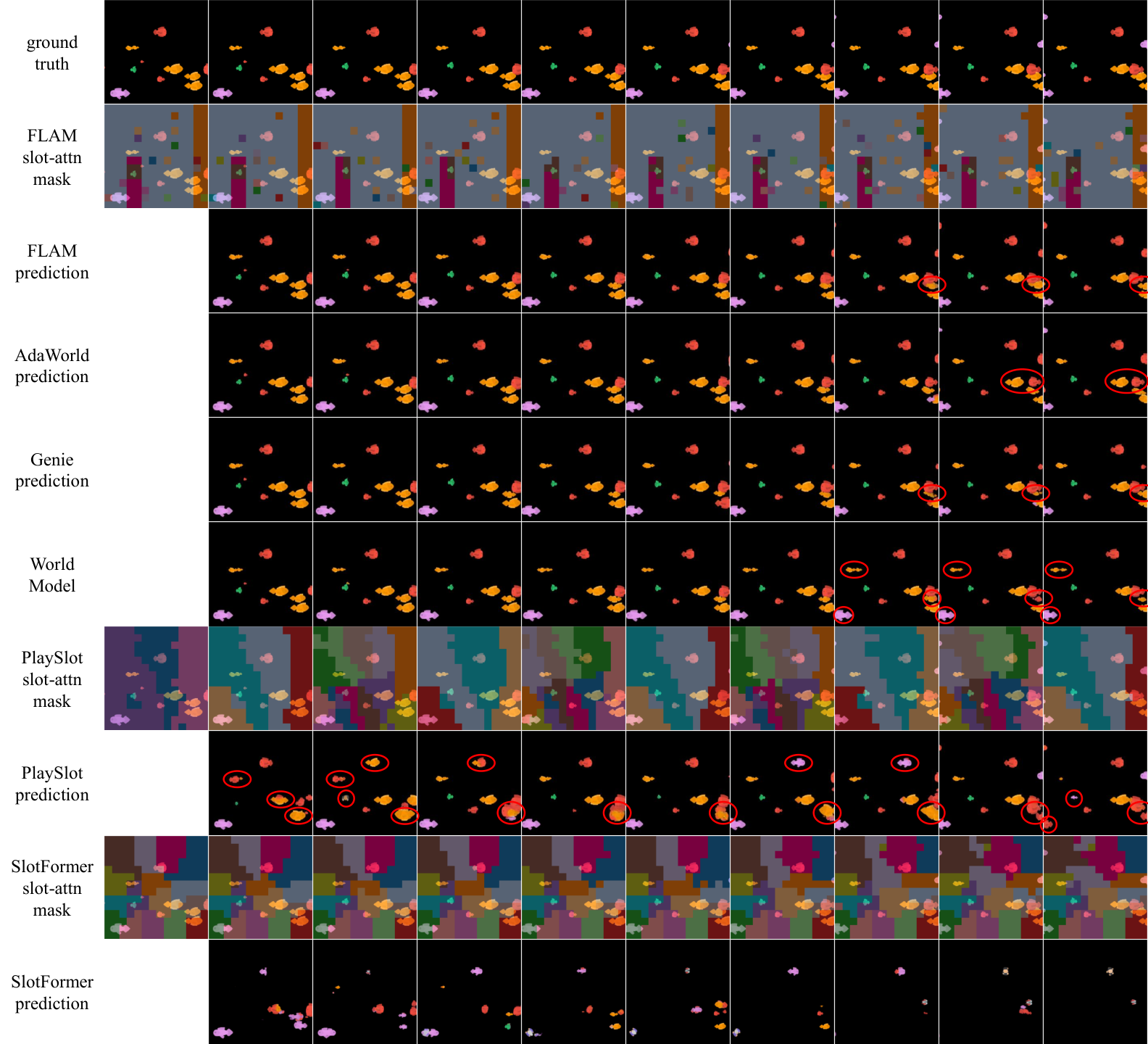
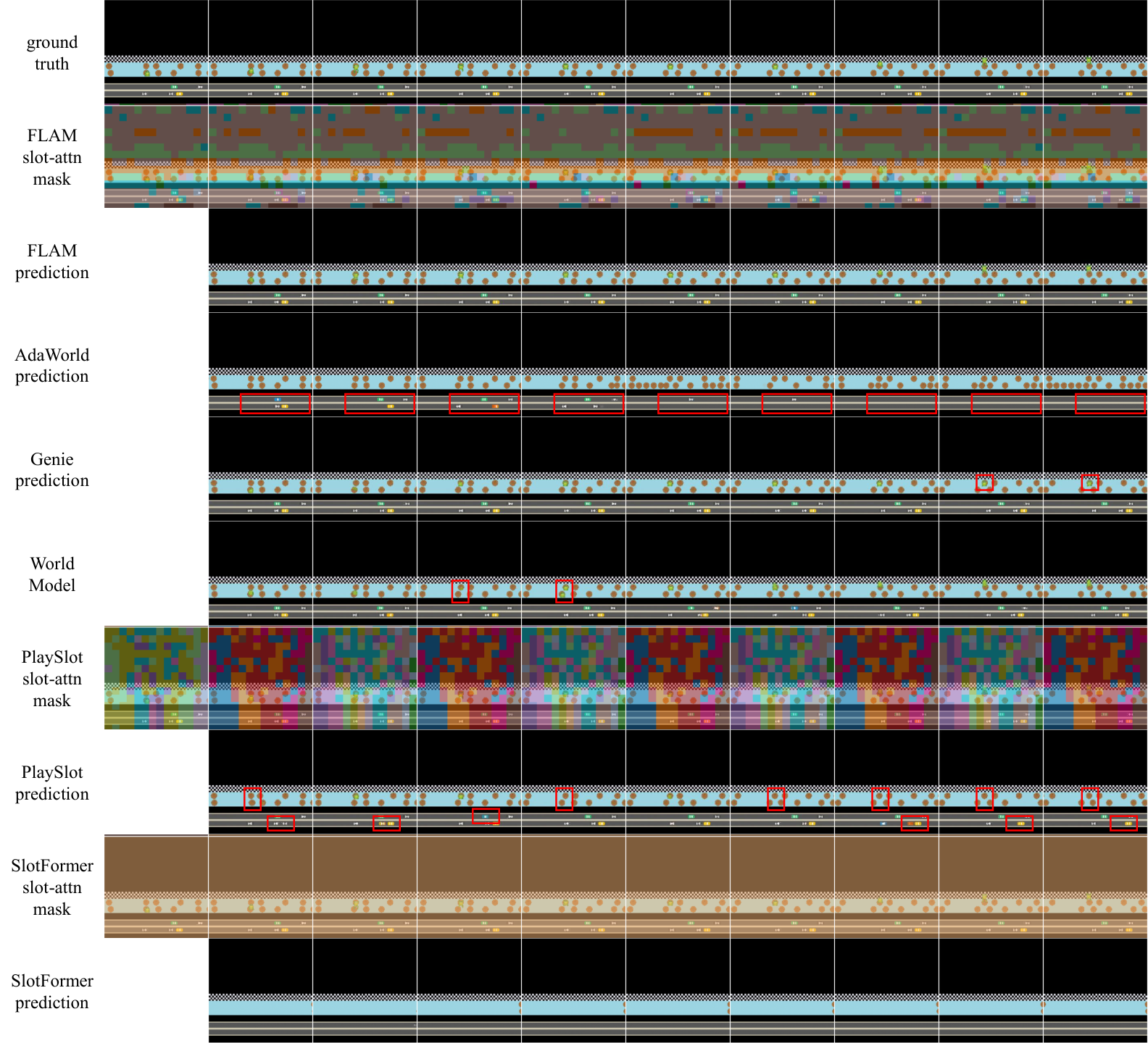
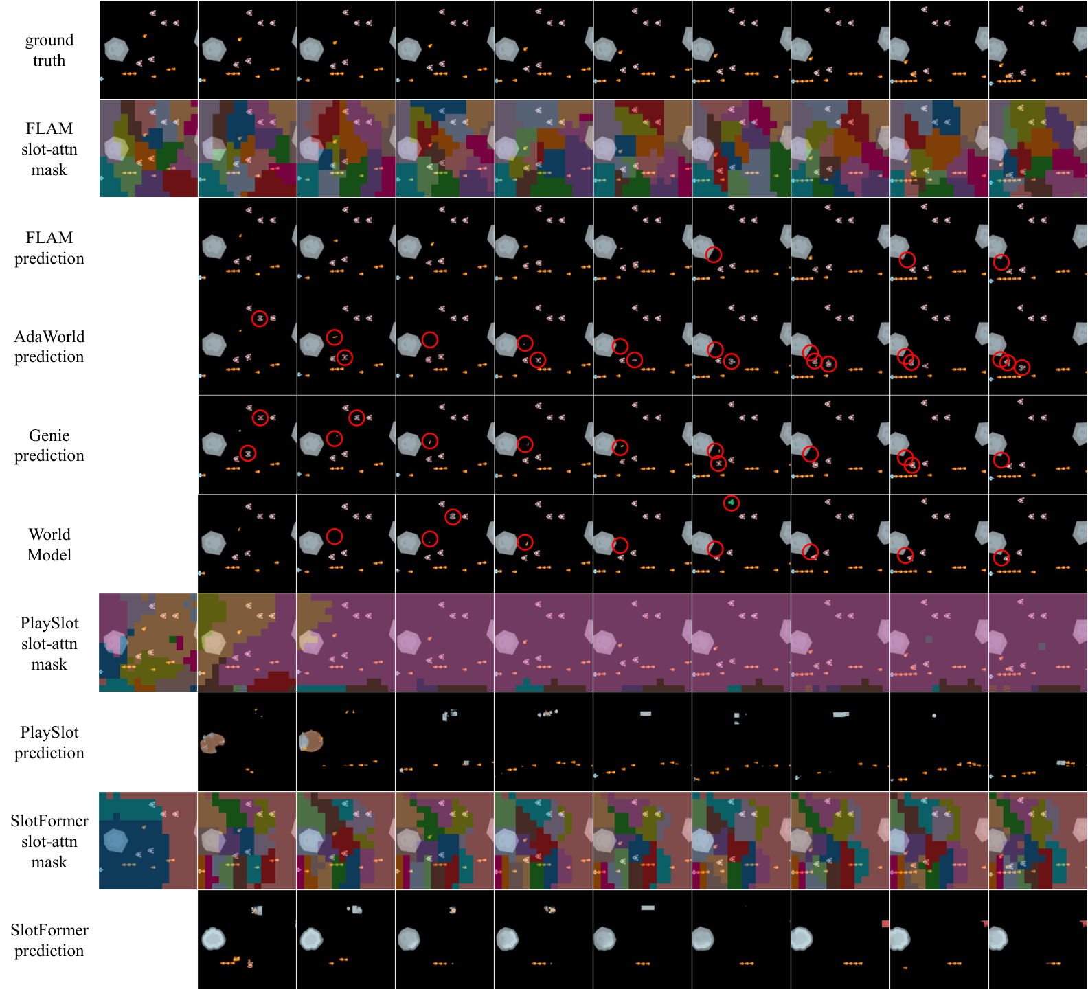
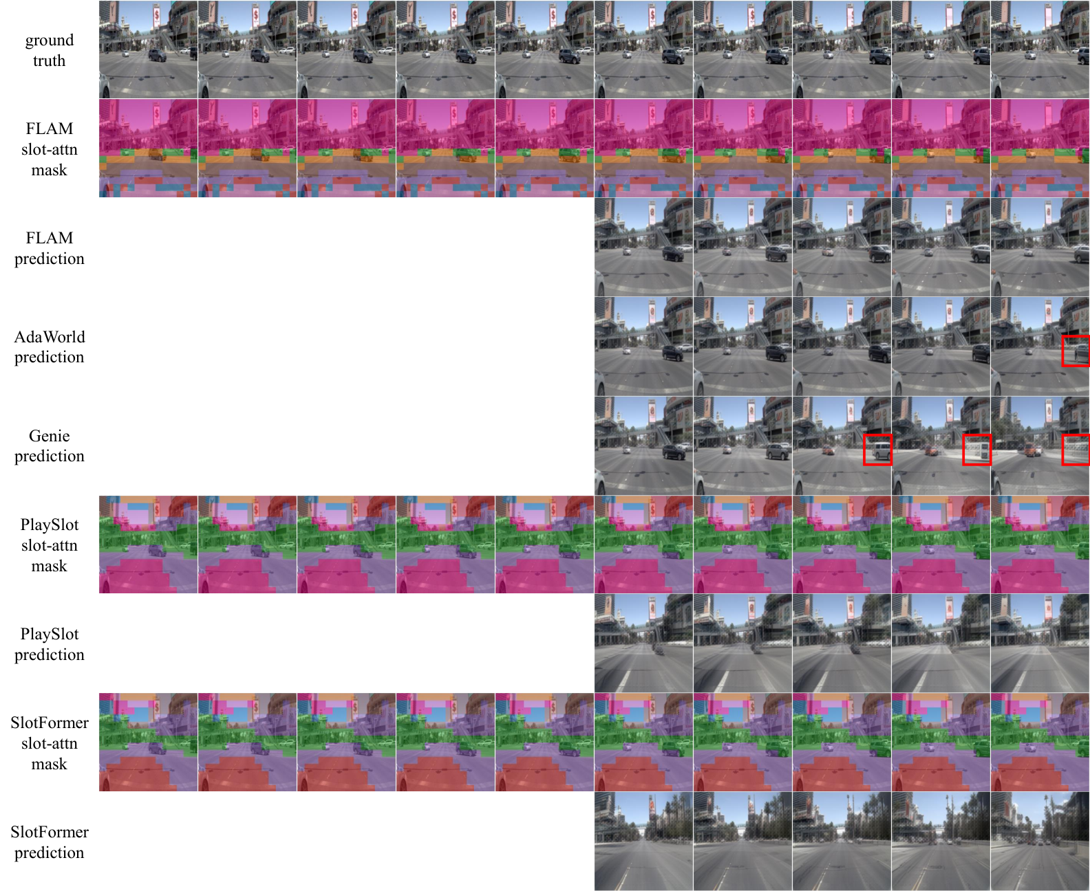
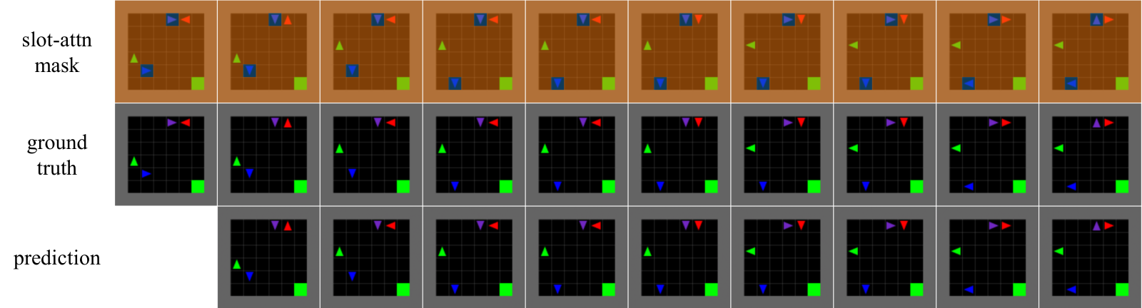
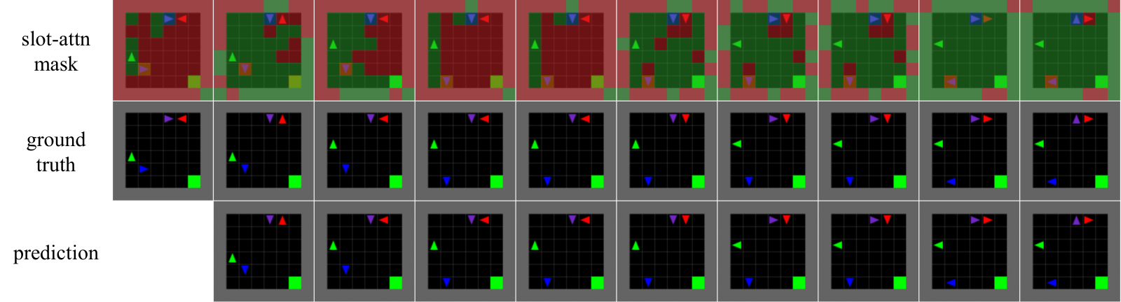
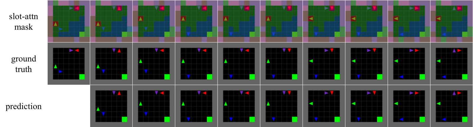
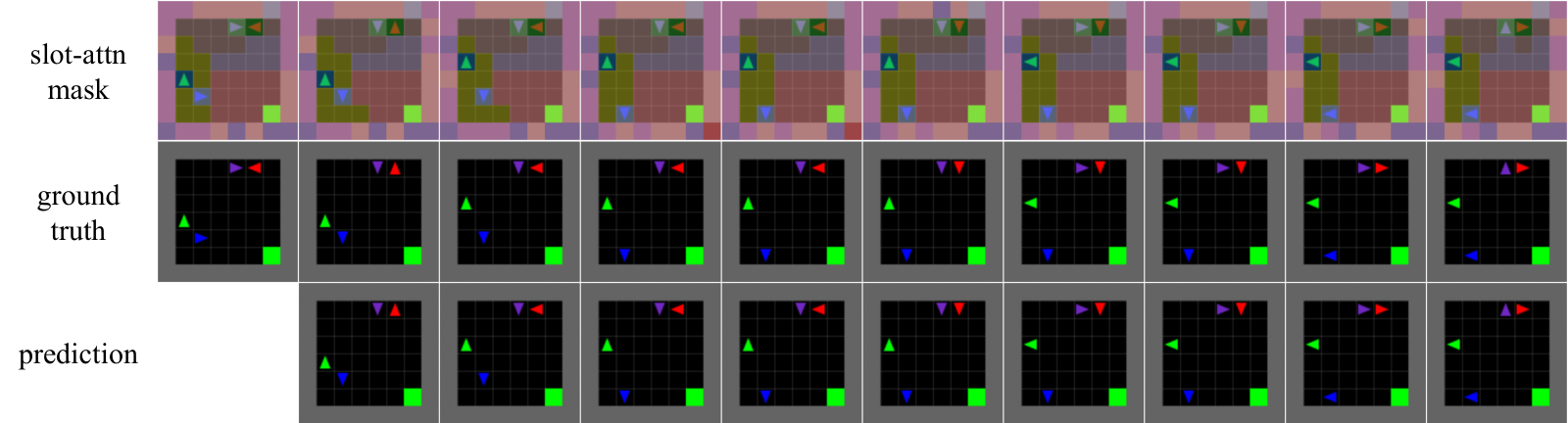
The appendix supplies qualitative prediction sequences, control edits, representation probes, policy-data details, and architecture/regularizer ablations. Every rollout panel, slot-binding mask, and marked prediction error is retained.
C.1 World Model Accuracy
World-model evaluation separates posterior-conditioned prediction accuracy from qualitative latent-control interventions. Both use the learned factorized model but support different claims.
Prediction Accuracy
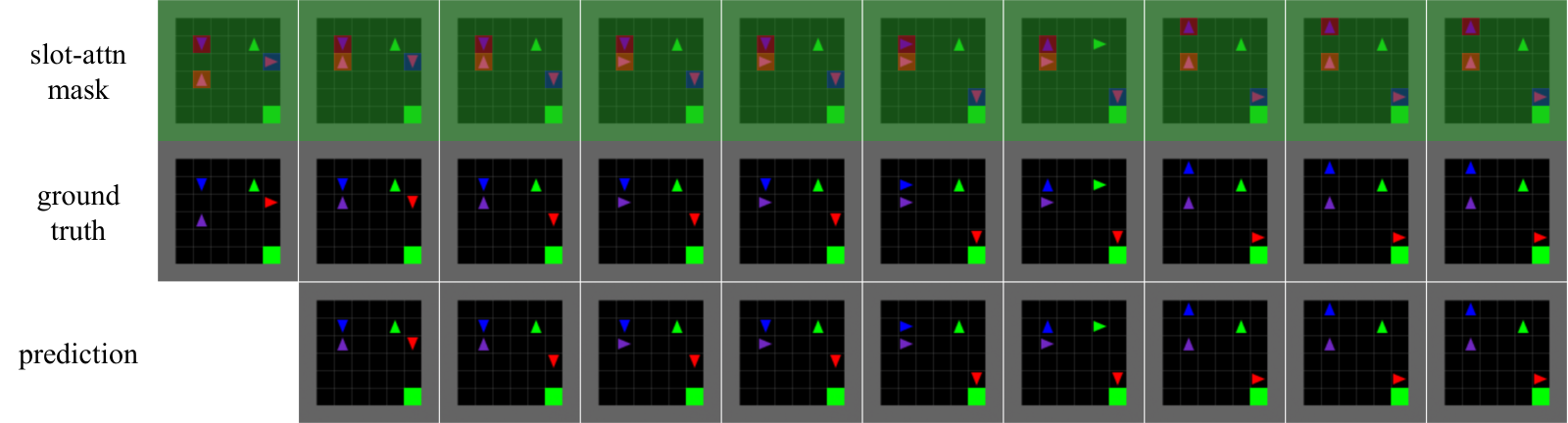
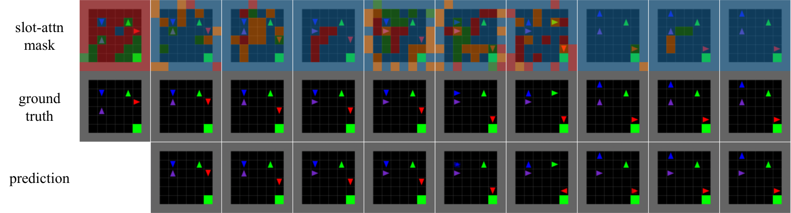
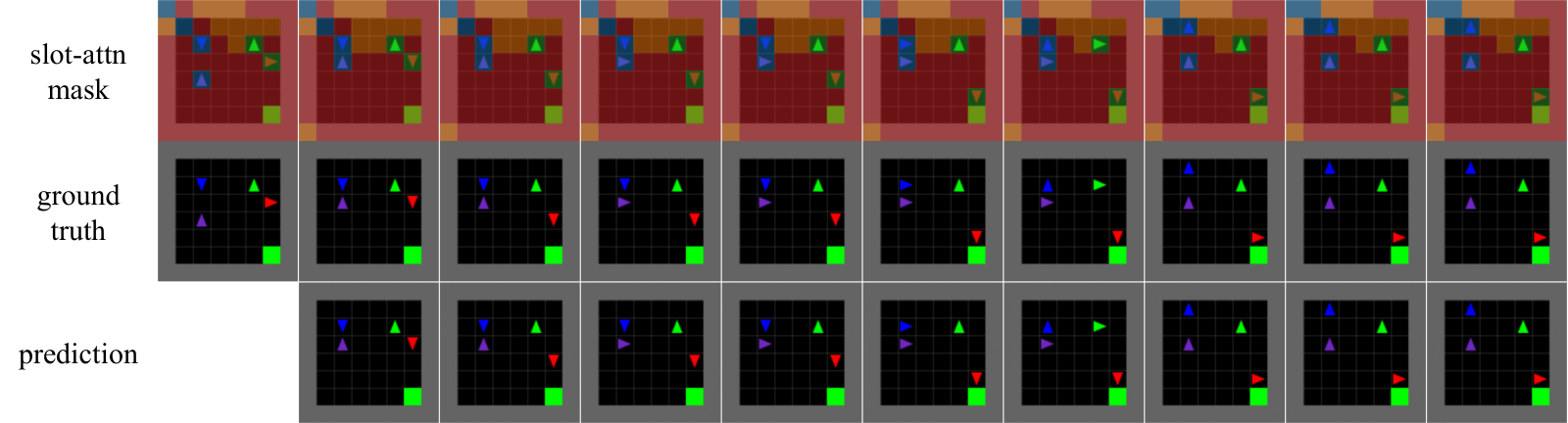
All datasets use ten-step autoregressive rollouts driven by actions inferred from the true video. Figures compare generated frames and slot-binding masks. Error annotations show remaining occlusion, projectile, and appearance failures even in FLAM, so accurate examples should not be read as perfect dynamics.
Scaling with the number of entities
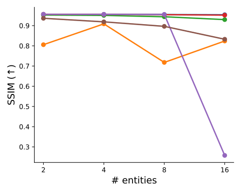
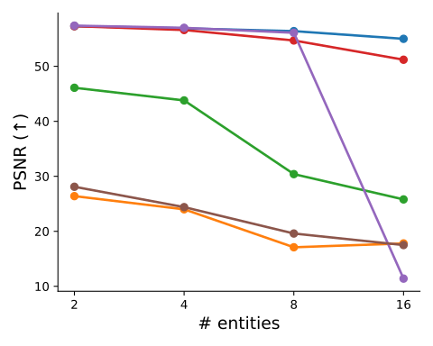
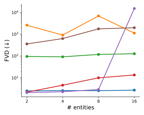
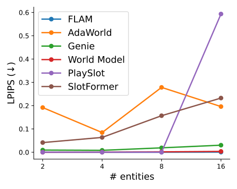
The MultiGrid scaling study varies entity count while matching total latent capacity against AdaWorld and matching Genie’s discrete capacity to joint combinations. For eight agents, FLAM uses eight thirty-two-dimensional actions and AdaWorld one 256-dimensional action. FLAM degrades less as the tested scene becomes more crowded; the evidence is an empirical grid-world comparison.
Controllable video generation
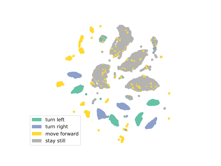
Control examples replace one entity’s latent actions while retaining the others’ inferred controls. A two-dimensional UMAP plot shows action-associated clusters. Forward motion blocked by an obstacle can overlap with staying still, because the visible transition is the same. This illustrates the distinction between inferred visual effects and uniquely recovering the command that caused them.




C.2 FLAM State Representation
Representation analysis measures whether factors separate independently acting agents and group deliberately correlated ones. The quantitative probe uses positions, while visualizations show binding masks and behavior over time.
Correlated Entities
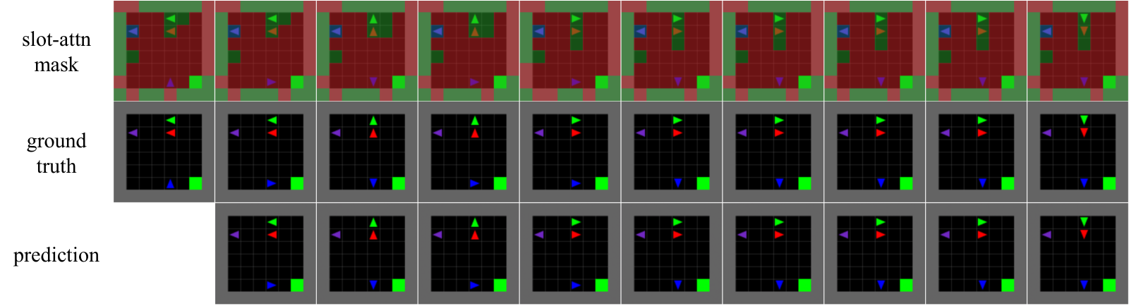
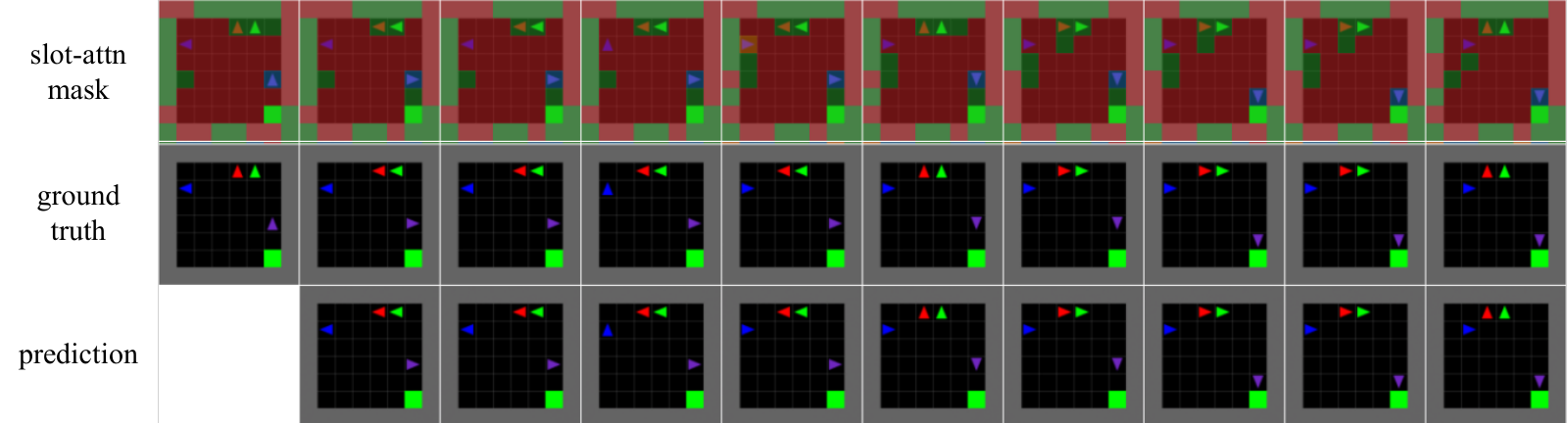
Two of four agents execute identical commands at every step, and three slots are available. Example rollouts show the correlated pair sharing a slot despite varying positions, supporting a role for common dynamics in grouping.
Independent Entities
A linear classifier predicts agent grid position from each slot. Hungarian matching minimizes position-label negative log likelihood to pair slots and agents during probe training. Normalized entropies of soft assignment probabilities define the adapted disentanglement and completeness scores; informativeness is matched position classification accuracy. Evaluation averages over slots/agents and held-out frames. The metrics are inspired by Eastwood and Williams, with this task-specific matching construction.
Equations 8
| (8) |
Number of factors K
Sweeping two, four, eight, and sixteen factors on four independent agents shows degradation when slots are insufficient and little prediction change once enough are available. Choosing enough slots for a varying population is a suggested practice; robustness beyond the tested counts and visual settings is not established.
C.3 Latent Action Policy Learning
Experts train with Phasic Policy Gradient for twenty-five million environment steps. Demonstrations for policy training, validation, and testing use disjoint Procgen levels, although the expert itself trains on all levels. FLAM-assisted and labeled-only cloning share the policy architecture and training setup; the former additionally uses inferred labels on the large demonstration set.
C.4 Ablation Studies
Ablations separately change temporal slot binding, access to other factors’ latent controls, and the strength of the latent bottleneck. Prediction and representation scores can move differently.
Factorizer architecture
Replacing factorizer temporal attention with previous-slot initialization makes bindings less consistent. FVD worsens from 2.9 to 36.6, while disentanglement/completeness/informativeness fall from 0.91/0.91/0.93 to 0.33/0.23/0.20. The retained rollout visualization shows the corresponding late-horizon failures.
Latent action model architecture
Global-Coupled FLAM gives each inverse prediction all next-frame slots and each forward prediction all latent actions. PSNR remains 56.3, near 56.5 for FLAM, but disentanglement falls to 0.79 and informativeness to 0.58. Completeness increases to 1.00, so the table does not show every representation score worsening. Accurate image prediction alone does not ensure separate entity-control channels.
| Metric | FLAM (ours) | FLAM w/o Factorizer Temporal Attention | Global-Coupled FLAM |
|---|---|---|---|
| PSNR () | 56.5 | 51.6 | 56.3 |
| SSIM () | 0.944 | 0.941 | 0.944 |
| LPIPS () | 3e-4 | 3e-3 | 4e-4 |
| FVD () | 2.9 | 36.6 | 3.72 |
| FLAM(ours) | FLAM w/o Factorizer Temporal Attention | Global-Coupled FLAM | Random | |
|---|---|---|---|---|
| D () | 0.91 | 0.33 | 0.79 | 0.32 |
| C () | 0.91 | 0.23 | 1.00 | 0.30 |
| I () | 0.93 | 0.20 | 0.58 | 0.10 |
KL regularization coefficient β
The KL penalty trades information capacity against prediction. Coefficients from 10⁻⁵ to 10⁻³ retain approximately 56.3–56.5 PSNR. At 10⁻², visual prediction degrades sharply. The default 2×10⁻⁴ lies within the successful tested range.
| Metric | ||||
|---|---|---|---|---|
| PSNR () | 56.5 | 56.5 | 56.3 | 24.9 |
| SSIM () | 0.944 | 0.944 | 0.944 | 0.911 |
| LPIPS () | 3e-4 | 3e-4 | 4e-4 | 0.057 |
| FVD () | 2.84 | 3.40 | 3.78 | 479.9 |