At a glance
Latent Forcing jointly denoises raw image pixels and pretrained visual features, giving each stream its own noise level. Generating the latent structure first provides an intermediate representation for subsequent pixel synthesis, while the final image comes directly from the pixel stream. On ImageNet at 256 × 256, this improves the tested pixel-transformer baselines at comparable model scale and training duration. It removes a separately trained image decoder but still relies on a pretrained feature encoder for training targets and, in guided sampling, an additional guidance model.
1 Introduction
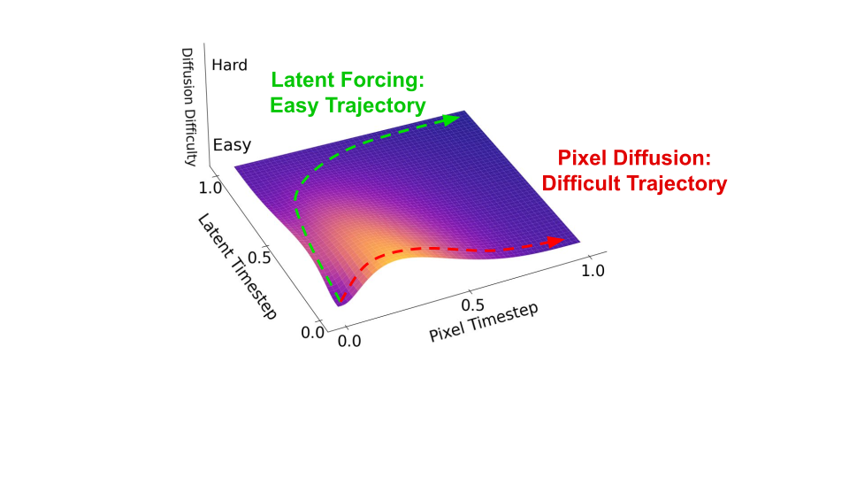
Latent diffusion makes image generation easier by modeling a compressed representation, but decoding can lose fine detail. Pure pixel diffusion avoids that reconstruction bottleneck yet follows the information ordering induced by noisy pixels. Latent Forcing separates these concerns: learn semantic structure early, then generate pixels without discarding original image information. Its claim is about useful generation order at the tested scale, rather than universal superiority to all latent or pixel architectures.
2 Related Work
The method builds on flow-based diffusion, latent-image models, and recent pixel transformers. JiT supplies direct clean-image prediction; REPA is the comparison for aligning diffusion representations with pretrained features. Unlike a separate latent decoder, the proposed model jointly predicts latent features and pixels. Unlike temporal diffusion forcing, its two streams describe the same image rather than an autoregressive sequence.
Related work also motivates noise scheduling and representation-conditioned generation. These connections frame the central experiment: whether ordering pretrained structure before pixels helps beyond merely adding a representation-alignment loss.
3 Ordering the Diffusion Process
Each modality receives its own time variable. Training can cover different pairs of noise levels, and inference follows a chosen monotone trajectory through that joint space.
3.1 Flow-Based Diffusion Review
The flow convention moves from Gaussian noise at time zero to clean data at time one. The model predicts the clean input and is trained with velocity-loss weighting, following JiT, rather than directly predicting a high-dimensional noisy target.
3.2 Flow on Multiple Tokenizers
A shared model predicts outputs for each noisy modality, with separate loss weights and possibly correlated noise times. At inference, modality-specific schedules determine how much each stream advances during a numerical integration step. Their relative signal-to-noise ratios describe the order in which information becomes available. Since the latent is a deterministic function of the image, keeping raw pixels in the modeled pair avoids a lossy image-reconstruction bottleneck; the paper expresses this through joint-distribution factorization, not an experimentally measured exact image likelihood.
Equations 1–3
| (1) |
| (2) |
| (3) |
3.3 Scaling as Time Scheduling
Scaling a modality changes its signal-to-noise ratio, which is equivalent to shifting its noise schedule. Combining differently scaled token spaces therefore chooses an implicit generation order even with a shared time variable. The retained time-shift equation makes this relation explicit.
Equation 4
| (4) |
4 Latent Forcing
Experiments instantiate the method as an ImageNet pixel diffusion transformer, principally using DINOv2 latents and 256 × 256 images.
4.1 Tokenization
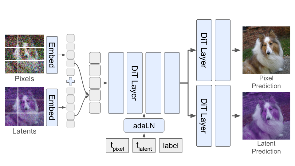
Pixels become 256 patches of dimension 768. Spatially aligned DINOv2 features, Data2Vec2 features, or lower-resolution pixels form the second stream. Pixel values are normalized to −1 through 1, and latent variance is matched to them. Sampling discards the generated features and rescales the predicted pixels, requiring no learned image decoder.
The pretrained feature extractor is a source of training targets and prior visual knowledge. Calling inference end to end does not mean the feature representations were learned from scratch jointly with this generator.
4.2 Architecture
Separate time embeddings and input/output projections accommodate the two streams. Their projected patch embeddings are added, keeping the transformer token count unchanged. An optional split of the last four layers into two two-layer output branches lets latent and pixel predictions specialize without adding layers or total stated operations. The standard experimental model is a large vision transformer trained for eighty epochs; the system comparison also uses two hundred epochs.
4.3 Prediction Target
The network predicts clean pixels and latents, then converts these predictions into velocity terms for the loss. Clipping the denominator near clean timesteps prevents numerical instability. The usual clipping constant is 0.05, with a different setting for the exploratory multi-schedule training.
Equation 5
| (5) |
4.4 Training Time vs Inference Time Ordering
The multi-schedule model independently samples each stream’s noise time, allowing one trained network to test different inference orders. The single-schedule model trains only around its selected trajectory, concentrating limited optimization on the intended sampling distribution. The former isolates ordering effects; the latter supplies the strongest baseline comparisons.
4.5 Multi-Schedule Diffusion
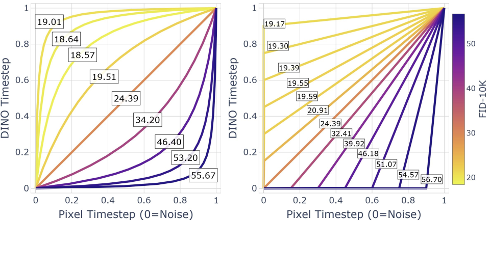
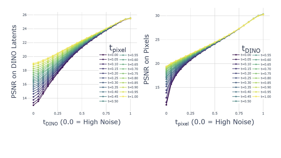
Exploratory training uses shifted uniform time sampling, a clipping constant of one third, and balanced latent/pixel loss magnitudes. Across DINOv2, Data2Vec2, and downsampled-pixel representations, denoising latent structure earlier is better than denoising full-resolution pixels earlier. For DINOv2, the unguided ten-thousand-sample distance drops from 55.35 with a strongly pixel-first shift to 18.65 with the tested latent-first shift of sixteen.
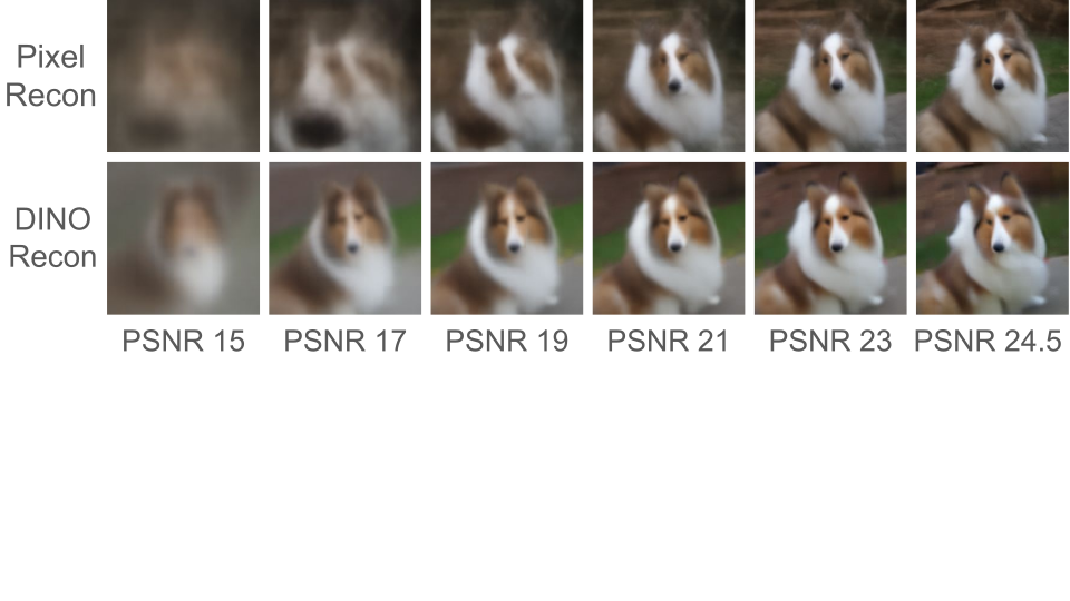
Matched-reconstruction-error examples show that latent-conditioned predictions preserve more recognizable spatial structure at early noise levels. The heat maps indicate that pixels help infer latents over much of the trajectory, while latent features add little to already mostly denoised pixels. These are diagnostic associations supporting the ordering explanation, not proof that one schedule is optimal for every dataset or model.
5 Single-Schedule Modeling
The remaining experiments commit training and inference to a particular order, primarily a cascade that generates latent features before pixels.
5.1 Time Sampling
Training first selects a latent or pixel phase. During a latent phase, pixels remain fully noisy and only latent loss is active; during a pixel phase, the latent is clean by default and only pixel loss is active. Separate logit-normal schedules choose the within-phase noise level. Balanced loss magnitudes and the probability of selecting each phase control the effective optimization allocation.
5.2 Improving Cascaded Generation
An additional early-pixel-time sample on 10% of updates improves the cascade modestly, as do separate output branches. Small noise added to latent conditioning during training addresses degradation seen with longer training: at two hundred epochs, the listed unguided score is 16.47 without this augmentation versus 10.93 with a maximum latent-noise amount of 25%. Adding noise during inference instead hurts. The interpretation is robustness to imperfect generated latents, rather than a rule to keep conditioning noisy during sampling.
| Model | FID Unguided |
|---|---|
| LF-DiT-L | 12.42 |
| Output Expert Layers | 12.93 |
| 10% Early Timesteps | 12.98 |
| Noise | FID |
|---|---|
| 0% | 10.93 |
| 5% | 11.07 |
| 10% | 11.46 |
| 15% | 11.81 |
| 25% | 12.55 |
5.3 Time Schedules
The tested cascade obtains ten-thousand-sample distances of 12.42 unguided and 6.60 guided, compared with 13.48/8.16 for a variance-shift trajectory and 20.98/10.73 for the selected linear offset. All use fifty Heun integration steps; the cascade allocates twenty-five to each phase. These numbers use a different sample count from the main fifty-thousand-sample comparisons and should not be mixed directly.
5.4 Guidance
The paper evaluates classifier-free guidance and AutoGuidance, which uses a smaller, weaker separately trained generator. AutoGuidance is strongest in most reported experiments. For the system-level comparison only, interval-restricted classifier-free guidance is used for latent steps and AutoGuidance for pixel steps. Guided scores therefore depend on extra model training and sampling configuration, not just the principal generator.
5.5 Distillation vs Ordering
At eighty epochs, conditional fifty-thousand-sample distance is 9.76 unguided for DINOv2 Latent Forcing, versus 18.60 for JiT with representation alignment and 25.18 for JiT alone. Guided values are 4.18, 4.57, and 5.64, a smaller separation. The controlled comparison supports an ordering benefit beyond representation distillation in this setup; it does not show that every use of distillation becomes ineffective.
| Model | FID Unguided | FID Guided |
|---|---|---|
| JiT | 25.18 | 5.64 |
| JiT+REPA | 18.60 | 4.57 |
| LF-DiT DINOv2 | 9.76 | 4.18 |
| LF-DiT D2V2 | 12.46 | 5.45 |
| Model | FID Unguided | FID Guided |
|---|---|---|
| JiT | 53.26 | 44.80 |
| JiT+REPA | 35.04 | 24.40 |
| LF-DiT DINOv2 | 20.44 | 13.36 |
| LF-DiT D2V2 | 20.99 | 15.56 |
| Model | Params | Dec. Params | Epochs | PSNR | FID(U) | FID(G) |
| Latent Diffusion | ||||||
| RAE | 839M | 415M | 800 | 18.09 | 1.51 | 1.13 |
| DiT-XL/2+SD-VAE | 675M | 49M | 1400 | 23.40 | 9.62 | 3.04 |
| SiT-XL/2+SD-VAE | 675M | 49M | 1400 | 23.40 | 8.3 | 2.62 |
| REPA+SD-VAE | 675M | 49M | 800 | 23.40 | 5.9 | 1.42 |
| MAR + Detok | 479M | 86M | 800 | 24.06 | 1.86 | 1.35 |
| LightningDiT | 675M | 41M | 800 | 25.29 | 2.17 | 1.35 |
| REPA-E | 675M | 41M | 1480 | 26.25 | 1.69 | 1.12 |
| MAR + UniFlow | 479M | 300M | 400 | 32.48 | 2.45 | 1.85 |
| Pixel Diffusion | ||||||
| ADM | 554M | 0 | 400 | 10.94 | 3.94 | |
| SiD UViT/2 | 2B | 0 | - | 2.77 | 2.44 | |
| SiD2 UViT/2 | - | 0 | - | - | 1.73 | |
| ViT Pixel Diffusion | ||||||
| JiT-L | 459M | 0 | 200 | 16.21 | 2.79 | |
| LF-DiT-L | 465M | 0 | 200 | 7.2 | 2.48 | |
5.6 Conditioning as Ordering
Unconditional models always receive the no-class label during training. DINOv2 Latent Forcing obtains 20.44 unguided and 13.36 guided, versus 35.04/24.40 for JiT with representation alignment and 53.26/44.80 for JiT. Data2Vec2 Latent Forcing also improves over the alignment baseline, despite a less extensively trained encoder. This shows the effect is not confined to one pretrained representation.
5.7 Discussion: Towards Rethinking Compression
At two hundred epochs, the 465-million-parameter model records 7.20 unguided and 2.48 guided, compared with 16.21/2.79 for 459-million-parameter JiT. Several larger, longer-trained latent models and other pixel architectures have better absolute guided scores. The supported result is improved performance among the compared plain pixel transformers at this compute scale. Infinite reconstruction signal-to-noise ratio refers to retaining the original pixels as input data, not perfect generated images. The retained system table separates decoder size, training duration, reconstruction quality, and generation distance.
6 Conclusion
Making generation order explicit improves the tested pixel-transformer models while retaining an uncompressed pixel output. The study is confined to ImageNet-256 and the reported architectures, schedules, and budgets; scaling to broader image distributions, text conditioning, or higher resolutions is not demonstrated. The main practical tradeoff is a simpler image-output path with additional latent targets, schedule choices, and guidance-model tuning.
7 Acknowledgments
The authors acknowledge National Science Foundation graduate fellowship support and discussion with Yue Zhao.
Appendix A Appendix
The appendix records architecture, optimizer and sampling settings, then details how guidance models and intervals were selected.
A.1 Implementation Details
The full configuration table is retained. The large model has twenty-four layers and hidden dimension 1,024; training uses Adam, batch size 1,024, learning rate 0.0002, five warmup epochs, and eighty or two hundred total epochs. Pixel and latent bottlenecks are 128-dimensional. The table separately specifies feature normalization, source encoders, loss weights, time samplers, and the fifty-step Heun sampler.
| ViT-S | ViT-B | ViT-L | |
| Architecture | |||
| Depth | 12 | 12 | 24 |
| Hidden Dim | 384 | 768 | 1024 |
| Heads | 6 | 12 | 16 |
| Patch Size | 16 | ||
| Pixel Bottleneck | 128 | ||
| Latent Bottleneck | 128 | ||
| Dropout | 0 | ||
| In-context CLS (Li and He, 2025) | 32 | ||
| In-context Start Block | 4 | ||
| Training | |||
| Epochs | 80 (ablation), 200 | ||
| Warmup Epochs | 5 | ||
| Optimizer | Adam (Kingma and Ba, 2014) | ||
| Adam Betas | |||
| Batch Size | 1024 | ||
| Learning Rate | 2e-4 | ||
| Learning Rate Schedule | constant | ||
| Weight Decay | 0 | ||
| EMA Decay | 0.9999 | ||
| Latent Sampler | |||
| Pixel Sampler | |||
| Class Token Drop | 0.1 | ||
| Sampling | |||
| ODE Solver | Heun | ||
| ODE Steps Total | 50 | ||
| ODE Steps Pixel (Cascaded) | 25 | ||
| ODE Steps Latent (Cascaded) | 25 | ||
| Global Time Steps | linear in [0.0, 1.0] | ||
| Pixels | |||
| Normalization | Linear Min-Max Rescaling | ||
| Standard Deviation (For Rescaling Sec 3.2) | 0.485 | ||
| Loss Weight (Eq. 1) | |||
| DINOv2 Latents | |||
| Normalization | Global norm to per each float, Following RAE (Zheng et al., 2025) | ||
| Model | DinoV2-Base + Registers (Oquab et al., 2023; Darcet et al., 2023) | ||
| Loss Weight (Eq. 1) | |||
| Layer | 12, Pre Norm, Following RAE (Zheng et al., 2025) | ||
| Data2Vec2 Latents | |||
| Normalization | Global norm to per each channel | ||
| Model | Data2Vec2-Large, 150ep (Baevski et al., 2023) | ||
| Loss Weight (Eq. 1) | |||
| Layer | 12 | ||
A.2 AutoGuidance
Four smaller guidance architectures are trained and checkpoint-swept. A small transformer with large-model output branches works best in the reported setting; its selected checkpoint is at epoch forty with exponential-moving-average decay 0.9995. Candidate checkpoints use two-thousand-sample evaluation and guidance schedules use eight-thousand-sample sweeps. AutoGuidance is also tested for JiT baselines but does not outperform their classifier-free guidance. This selection cost is additional to training the main model.
A.3 CFG on a Limited Interval
Only the system-level comparison uses interval guidance. Latent steps use classifier-free guidance strength 3 over the interval 0.06–1 and a time-shift factor 0.575; pixel steps use AutoGuidance strength 1.5 without an interval. Other reported experiments use AutoGuidance without interval restriction. Distinguishing these settings is necessary when comparing tables.