Overview
Intuition: a moving teacher and student can agree on useless constant speech features. This method gives them an additional acoustic reference: a fixed Gaussian mixture fitted to log-mel frames. The anchor supplies soft cluster probabilities rather than a single hard label. This January 2026 precursor is distinct from the later S-JEPA system, which changes both the target objective and how its mixture is updated.
At a glance
GMM-Anchored JEPA combines masked feature prediction with soft acoustic-cluster supervision. The cluster model is fitted once and remains fixed; its loss weight decays but retains a nonzero floor. Matched-architecture experiments compare speech recognition, emotion recognition and slot filling. The claim is improved stability and performance against these controlled baselines, not absolute leadership over every published speech model.
1 Introduction
Speech JEPA can collapse in the tested setup when the moving targets have no stable acoustic grounding. A frozen mixture over log-mel features supplies that reference without repeated offline reclustering. Keeping probabilities over several components preserves ambiguity near cluster boundaries. The contribution is best judged by whether this extra supervision prevents collapse and improves useful frozen features at matched compute.
2 Related Work
The paper contrasts contrastive speech learning, hard-cluster prediction and moving-teacher distillation. Their anti-collapse mechanisms and target sources differ. A fixed acoustic mixture is neither a semantic transcript nor a guarantee that its clusters correspond to phonemes.
3 Method
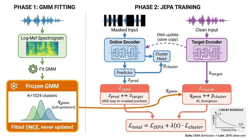
The method separates one-time acoustic clustering from joint encoder training. The decoder-free representation objective remains accompanied by an explicit fixed-target anchor.
3.1 Framework Overview
A fixed Gaussian mixture produces soft assignments from log-mel frames. During encoder training, one branch predicts moving-teacher features and another matches those fixed cluster probabilities. This combines adaptable latent targets with a stationary reference.
3.2 Phase 1: GMM Fitting
Diagonal-covariance mixtures keep fitting tractable and assign probability mass to several clusters for ambiguous frames. Because the input log-mel space does not change with encoder training, the anchor avoids a feedback loop in which both representation and cluster target drift together.
Equation 1
| (1) |
3.3 Phase 2: Joint Training
The objective adds masked feature regression to a cluster-distribution KL loss. The anchor starts strong and decays to a small positive value rather than disappearing. An ablation later shows that removing it entirely degrades this trained system, so the method is not an anchor-free JEPA after warmup.
Equations 2–4
| (2) |
| (3) |
| (4) |
3.4 Denoising Augmentation
The online encoder sees noise and mixed utterances while the teacher sees clean audio. Energy-based mixing defines the perturbation strength. This adds an invariance demand beyond simply predicting a missing interval.
Equations 5–6
| (5) |
| (6) |
3.5 Training Algorithm
The complete algorithm specifies teacher averaging, block masks and the anchor schedule. After training, the representation encoder is retained; the target branch and auxiliary supervision support training rather than ordinary feature extraction.
3.6 Architecture
The main encoder combines strided audio convolutions, density gates and a Conformer stack at 20 ms frames. A transformer variant checks whether the anchor’s benefit depends on that backbone. The controlled WavLM-style baseline uses the same architecture, unlike an unrestricted comparison with published WavLM checkpoints.
4 Experiments
Models are trained on about 50,000 hours of English audio and evaluated using frozen encoders with task-specific heads. The matched WavLM-style comparison isolates objective changes better than comparisons across unrelated pretrained systems. Recognition uses the specified labeled downstream data and greedy decoding; those supervised heads are not part of pretraining.
| Model | WER (%) | CER (%) | WER |
|---|---|---|---|
| Pure JEPA | 100.00 | 93.11 | – |
| WavLM-style | 33.22 | 11.28 | baseline |
| GMM-JEPA | 29.18 | 9.62 | 12.2% |
| GMM-JEPA-T | 28.68 | 9.44 | 13.7% |
| Model | Type F1 | Edit F1 | Type |
|---|---|---|---|
| Pure JEPA | 5.0 | 2.2 | – |
| WavLM-style | 59.1 | 33.7 | baseline |
| GMM-JEPA-T | 59.2 | 32.8 | 0.1 |
| GMM-JEPA | 64.7 | 36.0 | 5.6 |
| Model | F1 | F2 | F3 | F4 | F5 | Avg | |
|---|---|---|---|---|---|---|---|
| Pure JEPA | 48.88 | 46.12 | 49.89 | 48.67 | 46.97 | 48.11 | – |
| WavLM-style | 64.83 | 64.19 | 65.30 | 67.11 | 65.85 | 65.46 | base |
| GMM-JEPA | 66.07 | 67.85 | 66.67 | 68.56 | 67.37 | 67.30 | 1.8 |
| GMM-JEPA-T | 67.19 | 67.52 | 67.58 | 68.11 | 68.41 | 67.76 | 2.3 |
5 Analysis
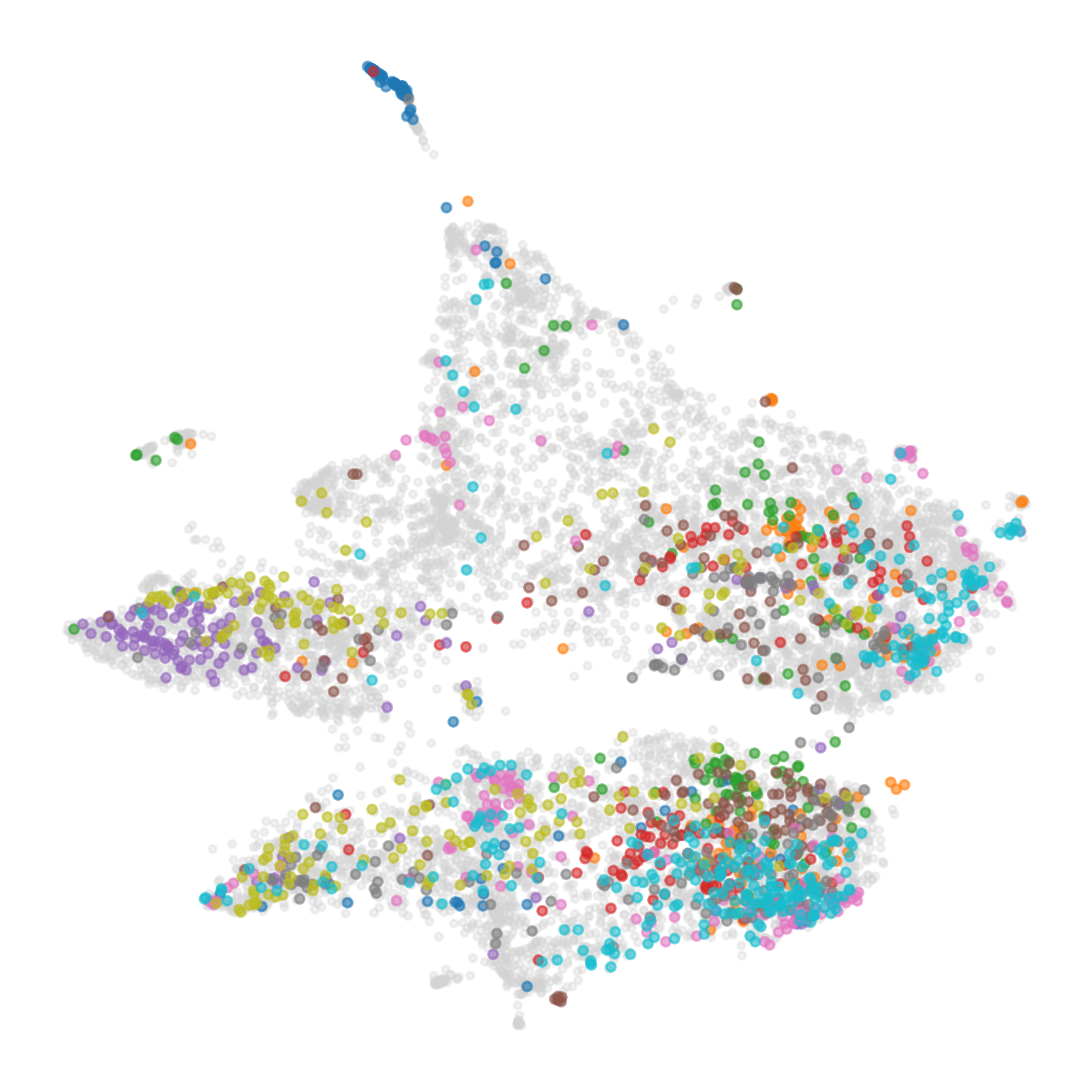
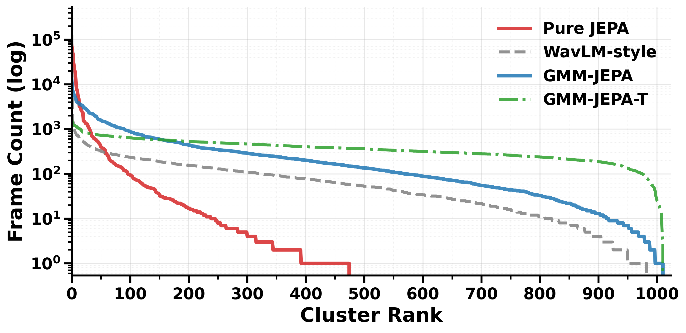
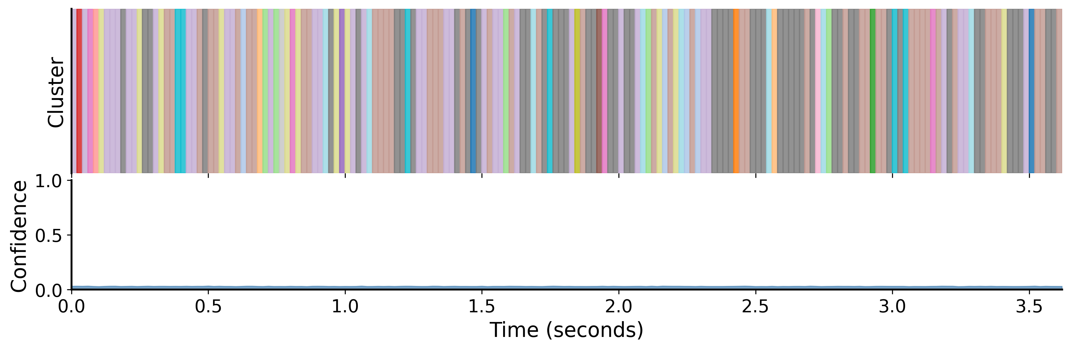
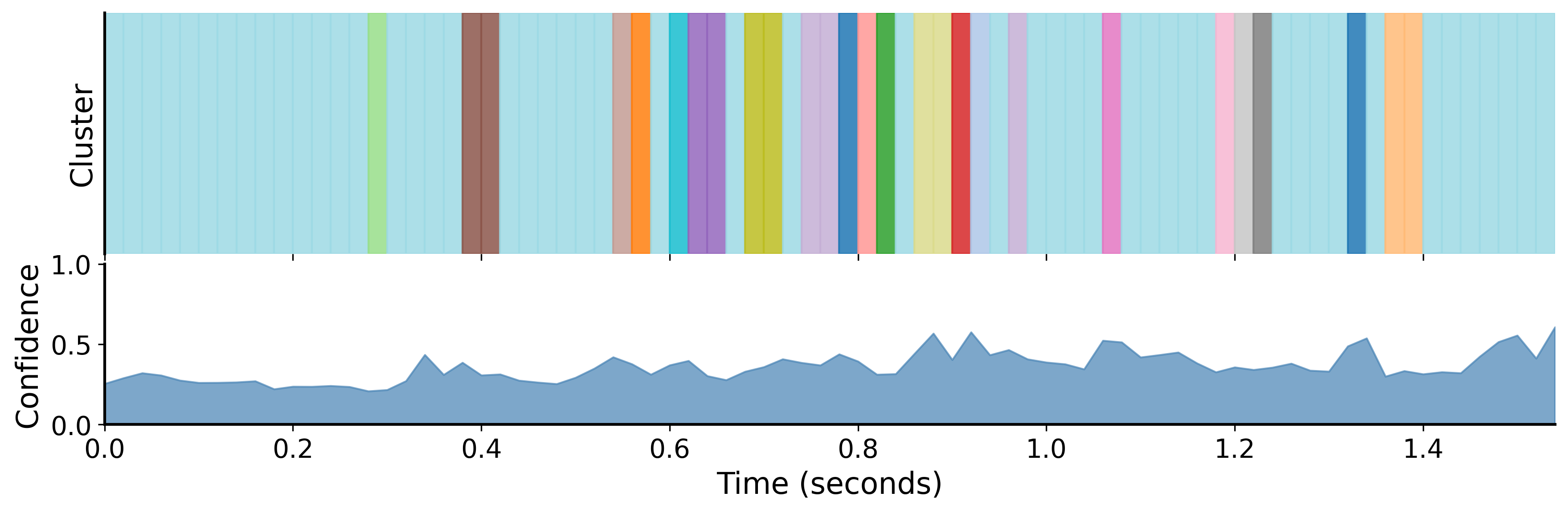
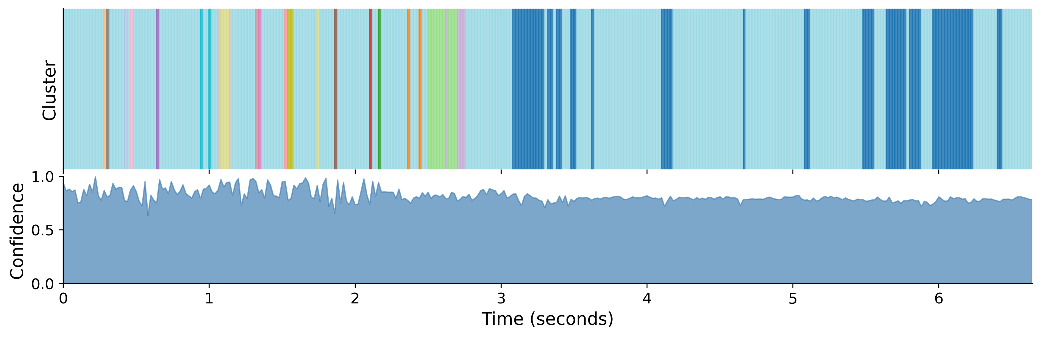
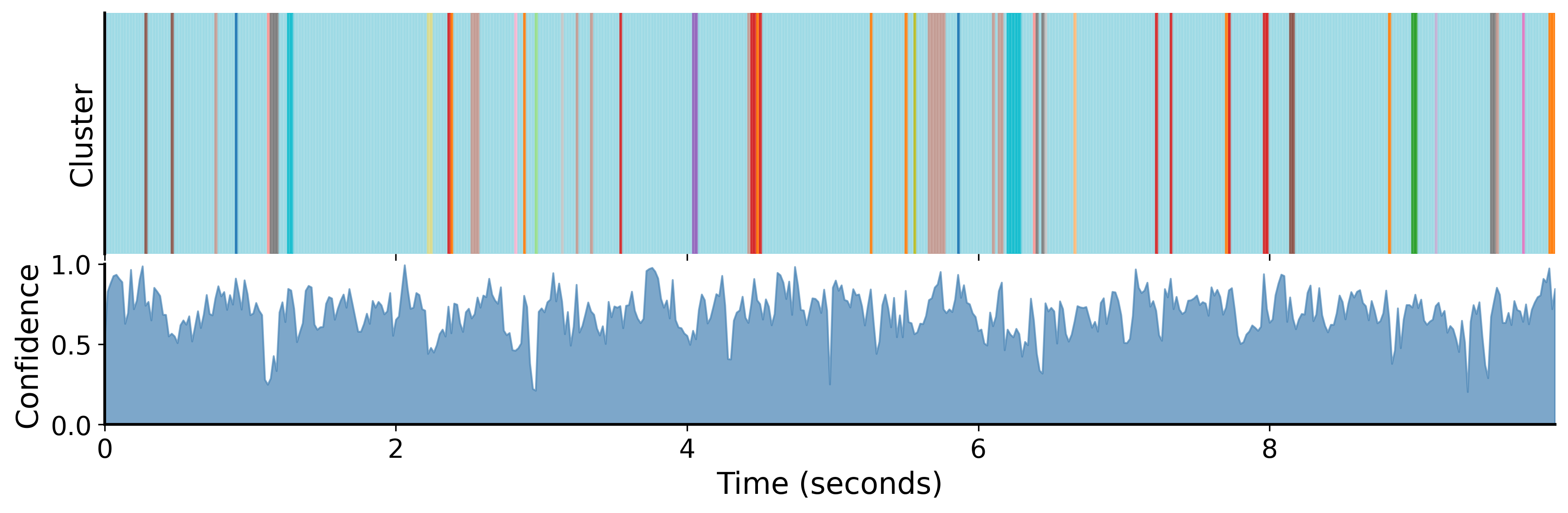
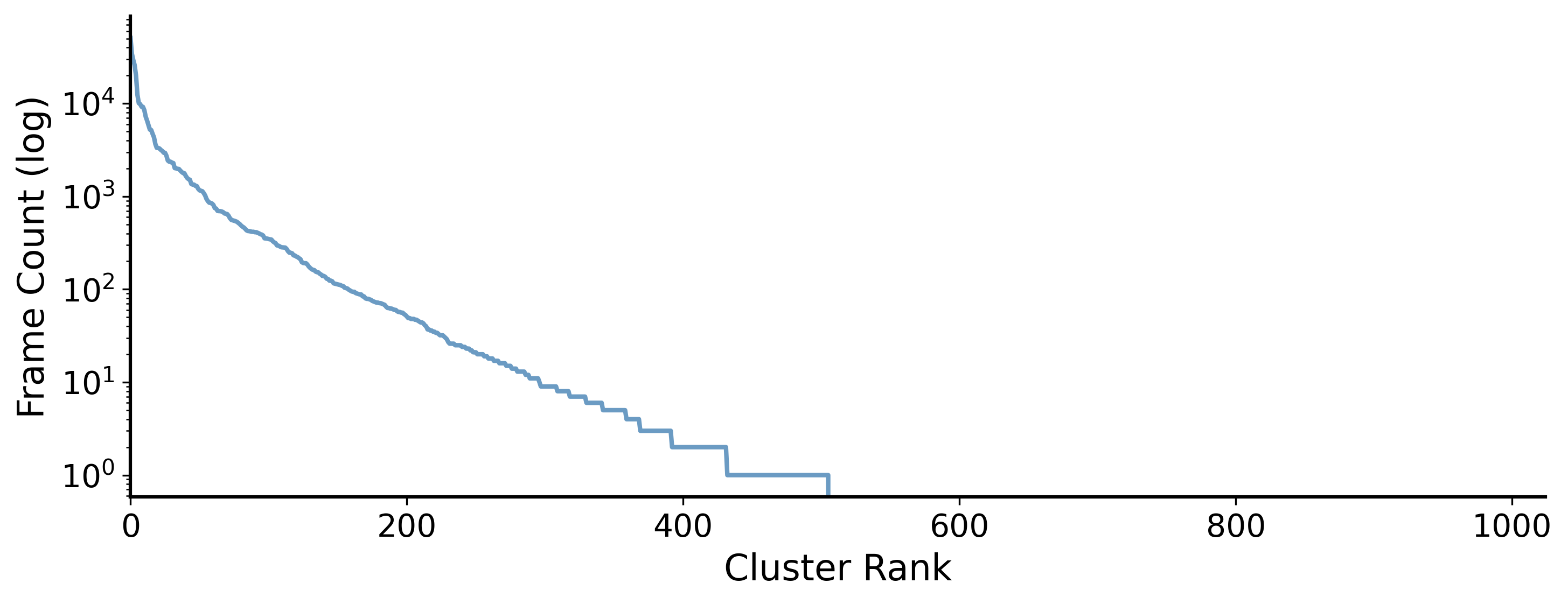
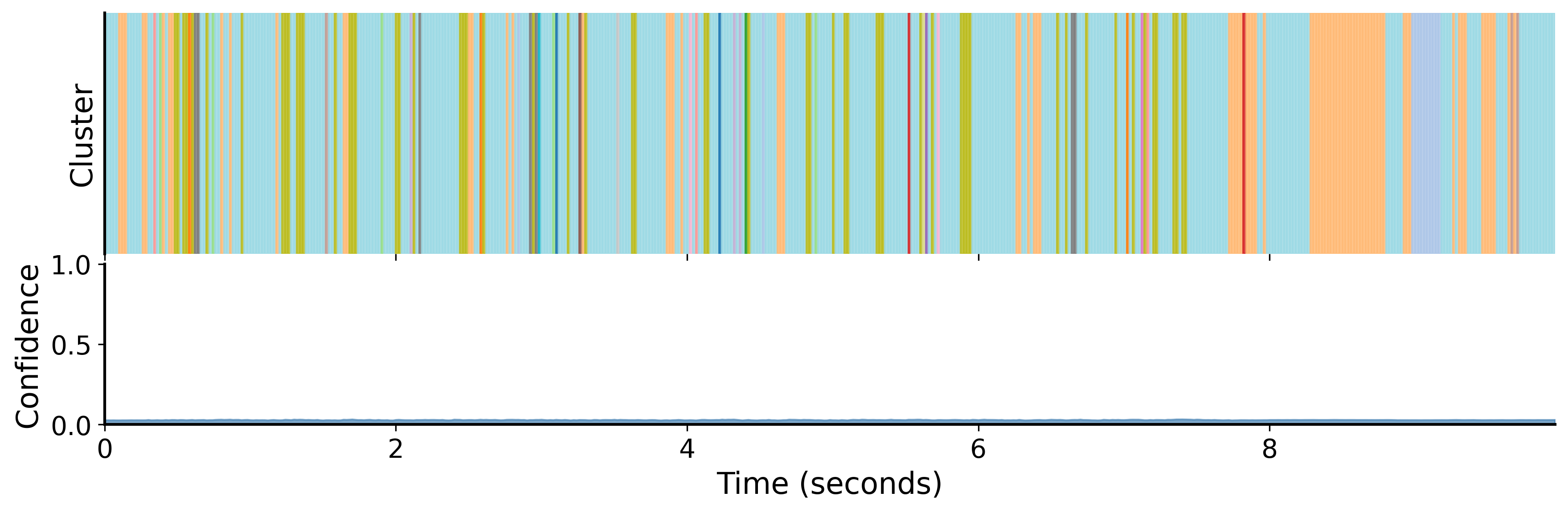
Cluster-use entropy measures whether many categories are used, while adjacent consistency measures temporal smoothness. A high value of either alone is insufficient: uniform random categories can have high entropy, and a constant output can be perfectly smooth. The combination of diagnostics and downstream tasks is therefore more informative than a single visualization.
Equations 7–8
| (7) |
| (8) |
5.1 Embedding Quality Analysis
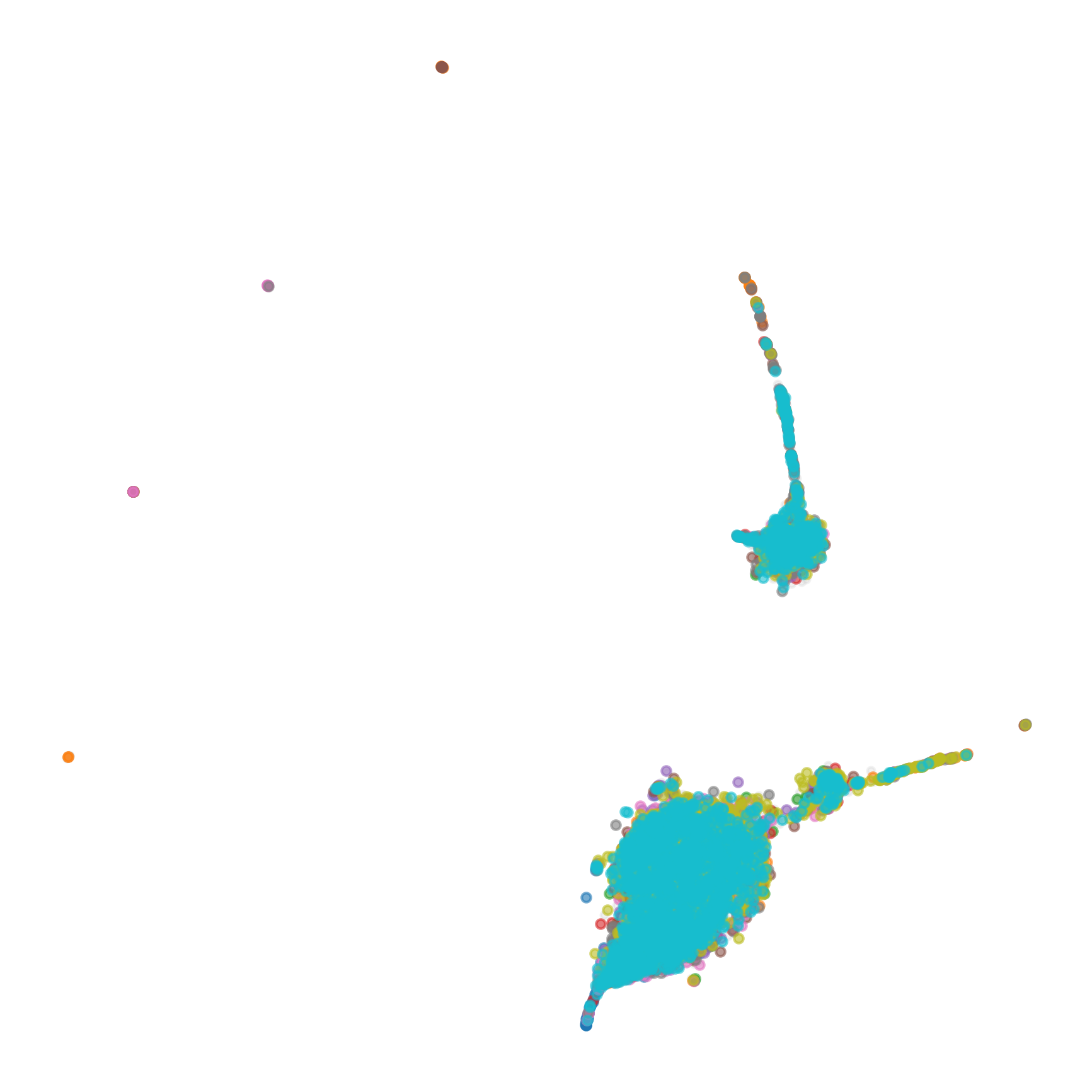
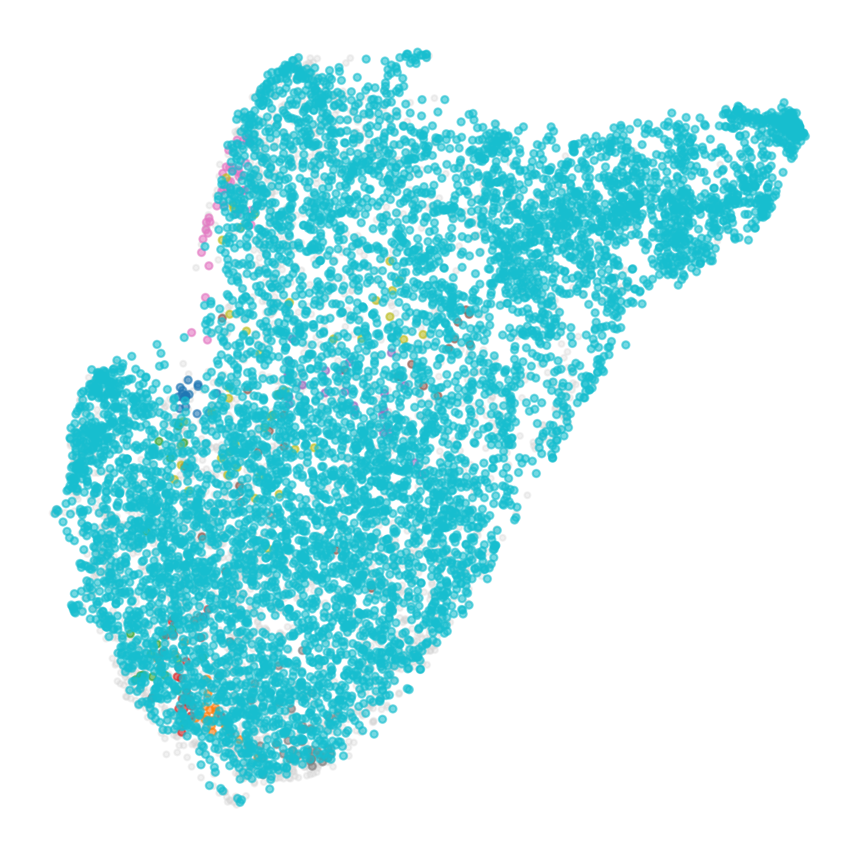
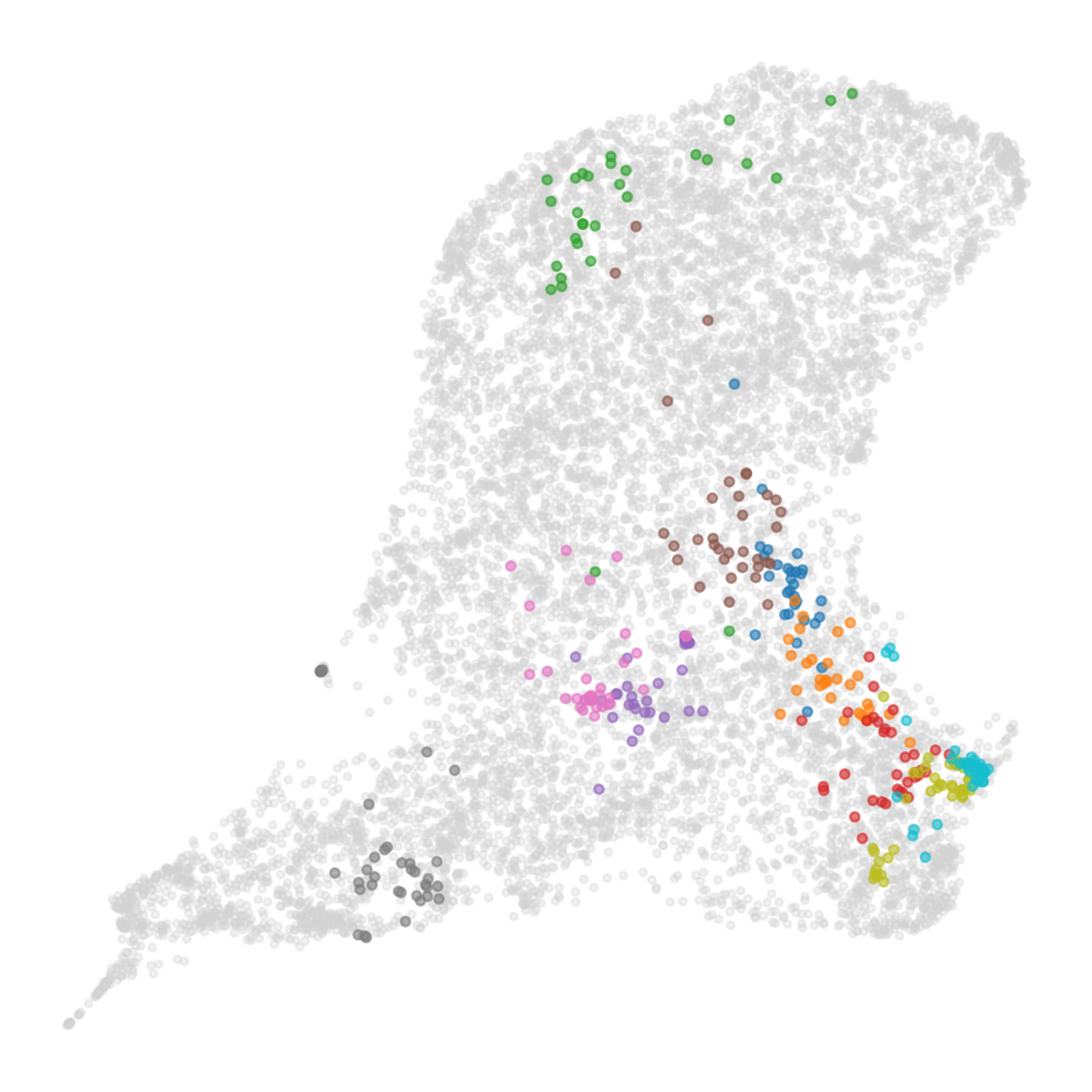
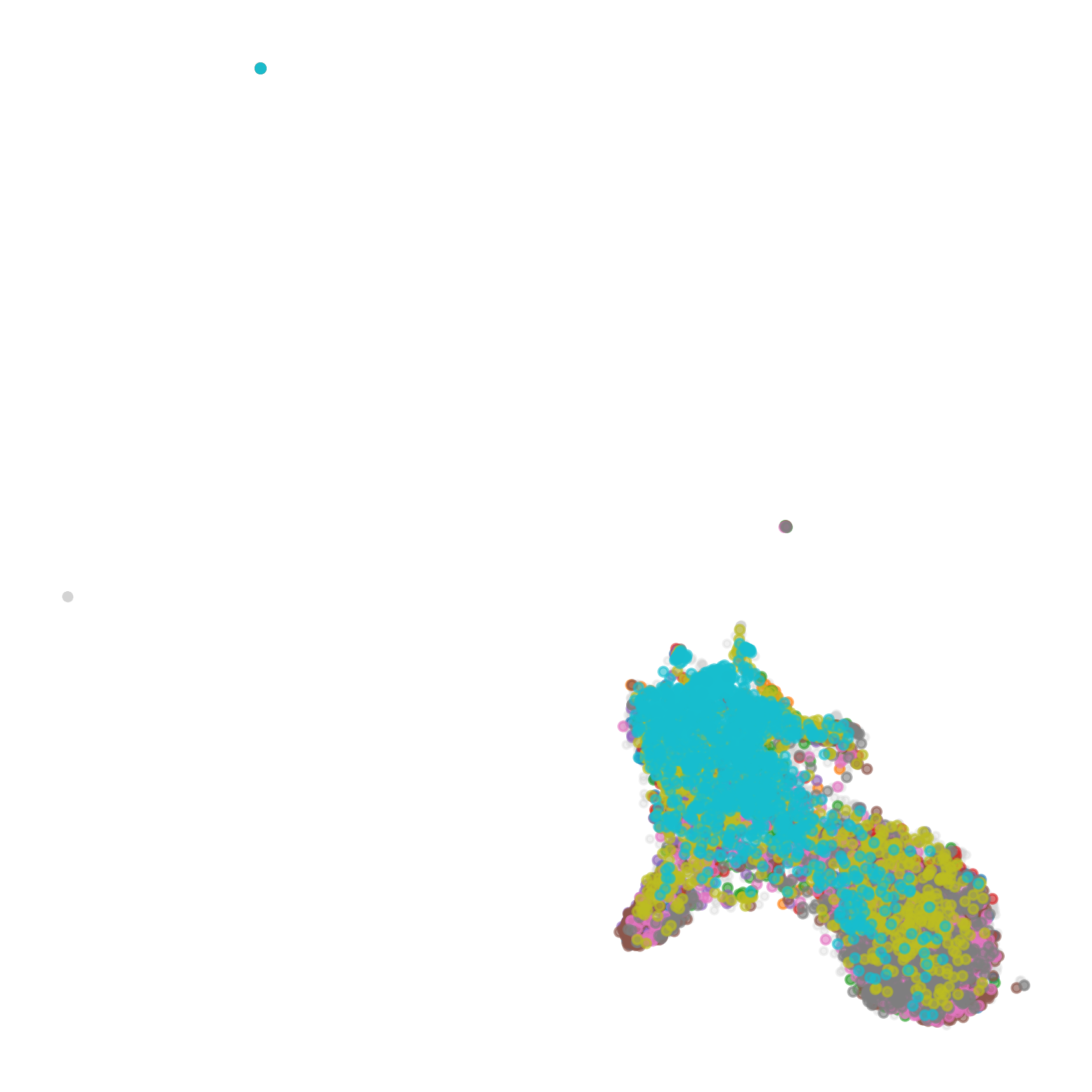
The study combines cluster agreement, linear and nonlinear probes, and label alignment. Some features favor speaker or gender information while others favor phonetic distinctions. Probe success measures recoverability under a trained readout, not a transcript already present in the unsupervised cluster IDs.
Equation 9
| (9) |
| Model | Speaker | Gender |
|---|---|---|
| Pure JEPA | 18.71.8 | 69.21.5 |
| WavLM-style | 99.60.3 | 99.40.2 |
| GMM-JEPA-T | 99.70.2 | 99.70.2 |
| GMM-JEPA | 99.80.2 | 99.60.3 |
| Model | Linear | MLP |
|---|---|---|
| Pure JEPA | 7.40.0 | 9.00.1 |
| WavLM-style | 47.60.2 | 57.50.2 |
| GMM-JEPA-T | 51.40.1 | 59.40.4 |
| GMM-JEPA | 53.00.1 | 64.20.2 |
5.2 Ablation: GMM Anchoring
When the anchor coefficient decays to zero, cluster utilization and downstream results worsen. This supports retaining the residual fixed-target loss in the tested recipe. It does not establish that every JEPA speech architecture requires this particular mixture or schedule.
6 Discussion
The discussion interprets the acoustic anchor as a practical stabilizer. Limits include the fixed feature space, mixture-model assumptions, English data and the need to test larger scales and other acoustic domains. The controlled baseline results should remain separate from claims about absolute state of the art.
7 Conclusion
The method demonstrates that a one-time soft acoustic clustering can support useful latent prediction without repeated offline reclustering. Its gains concern the evaluated backbones and tasks. The later S-JEPA formulation is a continuation of this line, not merely another title for this exact objective.
Impact Statement
The impact statement concerns speech-model research broadly. The reported representation metrics do not themselves assess privacy, demographic fairness or deployment reliability.
Appendix A Architecture Details
The appendix fixes the architecture shared by the main model and its controlled baseline. These details are needed to distinguish an objective comparison from a backbone comparison.
A.1 Encoder Backbone
The encoder uses strided convolutional blocks before the Conformer. This establishes frame resolution and local receptive fields before attention.
Equations 10–14
| (10) |
| (11) | ||||
| (12) | ||||
| (13) | ||||
| (14) |
A.2 Snake-Beta Activation
Snake-Beta supplies a learnable periodic component to the nonlinear activation. Its presence is a shared architectural choice rather than the isolated GMM-anchoring contribution.
Equation 15
| (15) |
A.3 Gated Relative Position Bias
Gated relative-position bias adjusts attention scores according to distance and learned gates. The complete equations preserve how positional information enters the Conformer.
Equations 16–20
| (16) |
| (17) | ||||
| (18) |
| (19) | ||||
| (20) |
A.4 Layer Aggregation
Cross-attention aggregates intermediate layers into a representation. Learned layer combination can preserve information at several depths; it should not be confused with selecting a transcript-aligned acoustic unit.
Equations 21–25
| (21) | ||||
| (22) | ||||
| (23) | ||||
| weights | (24) | |||
| (25) |
A.5 Density Adaptive Attention (DAAM)
The density-adaptive gate normalizes temporal features and combines Gaussian-mixture responses before modulation. This gate is distinct from the frozen acoustic GMM that supplies the auxiliary training target.
Equations 26–29
| (26) |
| (27) | ||||
| (28) |
| (29) |
A.6 Cluster Prediction Head
The cluster head maps encoder features to a distribution over the fixed mixture components. It learns to match soft probabilities rather than force each frame into a single label.
Equations 30–32
| (30) | ||||
| (31) | ||||
| logits | (32) |
A.7 Predictor Architecture
The predictor estimates teacher features at hidden positions from context. It supports the latent-regression part of the objective, separately from cluster-distribution supervision.
A.8 Target Encoder and EMA Update
The averaged target encoder supplies slowly changing latent targets. Its averaging coefficient controls lag and does not by itself supply the stationary acoustic reference.
Equation 33
| (33) |
Appendix B Training Hyperparameters
The full hyperparameter table records masking, schedules, optimization and architecture settings for the reported runs. These values describe the experiment; they are not claimed as universally optimal speech settings.
| Conformer | Transformer | |
| Encoder Architecture | ||
| Parameters | 31.1M | 41.3M |
| CNN layers | 3 | 7 |
| Channels | [32,64,128,256] | [256]7 |
| Strides | [8,8,5] | [5,2,2,2,2,2,2] |
| Latent dim | 512 | 512 |
| Encoder layers | 4 | 10 |
| Attention heads | 32 | 8 |
| FFN mult / dim | 4512 | 2048 |
| Conv kernel | 31 | – |
| GMM Fitting | ||
| Components | 1024 | |
| Mel bins | 80 | |
| Initialization | K-means++ | |
| Optimization | Mini-batch SGD | |
| Learning rate | (cosine) | |
| Training frames | 9.6B | |
| K-Means Fitting (WavLM-style baseline) | ||
| Components | 1024 | |
| Feature type | Log-mel (80 bins) | |
| Initialization | K-means++ | |
| Update method | Lloyd’s algorithm | |
| Lloyd iterations | 20 | |
| Training frames | 9.6B | |
| Training | ||
| Optimizer | AdamW [22] | |
| Learning rate | ||
| LR schedule | linear warmup / decay | |
| Weight decay | ||
| Micro Batch size | 96 (Conformer) | 192 (Transf.) |
| Gradient clipping | 1.0 | |
| GPUs | 8 B200 | |
| EMA | 0.996 | |
| decay | ||
| Mask ratio | ||
| Span length | frames | |
| Augmentation | ||
| Noise SNR | dB | |
| Mix ratio | dB | |
| Noise/mix prob. | 0.25 each | |
Appendix C GMM Details
The mixture appendix specifies how acoustic features become probabilistic cluster targets. It is the fixed anchor’s implementation contract.
C.1 Posterior Computation
Posterior probabilities combine each component’s likelihood with its mixture weight and normalize across components. Diagonal covariance and variance floors constrain the statistical model and numerical behavior.
Equation 34
| (34) |
C.2 Chunked Soft Assignment
Chunking the assignment calculation bounds memory without changing the target probability distribution. The preserved algorithm retains how chunks are accumulated.
Appendix D Augmentation Details
Noise and overlap augmentation are defined by waveform energy so their strength has a consistent acoustic interpretation.
D.1 Energy-Based SNR Mixing
The noise scale is chosen from a target signal-to-noise ratio using clean and noise energies. The exact sampling range remains in the source equations.
Equations 35–37
| (35) | ||||
| (36) | ||||
| (37) |
D.2 Utterance Mixing
A segment from another utterance is scaled and mixed into the primary waveform. This is acoustic augmentation, not an independent semantic label for the mixed speech.
D.3 Augmentor Buffer
The augmentor buffer supplies reusable noise or utterance segments. Its role is practical data mixing; the attached fold-level result table is retained in its original location.
Appendix E Visualization Details
UMAP projection settings document the visual comparison. Such projections illustrate cluster organization but cannot establish high-dimensional separation or downstream quality without the quantitative tests.
| Parameter | Value |
|---|---|
| n_neighbors | 15 |
| min_dist | 0.1 |
| metric | Euclidean |
| n_components | 2 |
| random_state | 42 |
| n_samples | 10,000 |