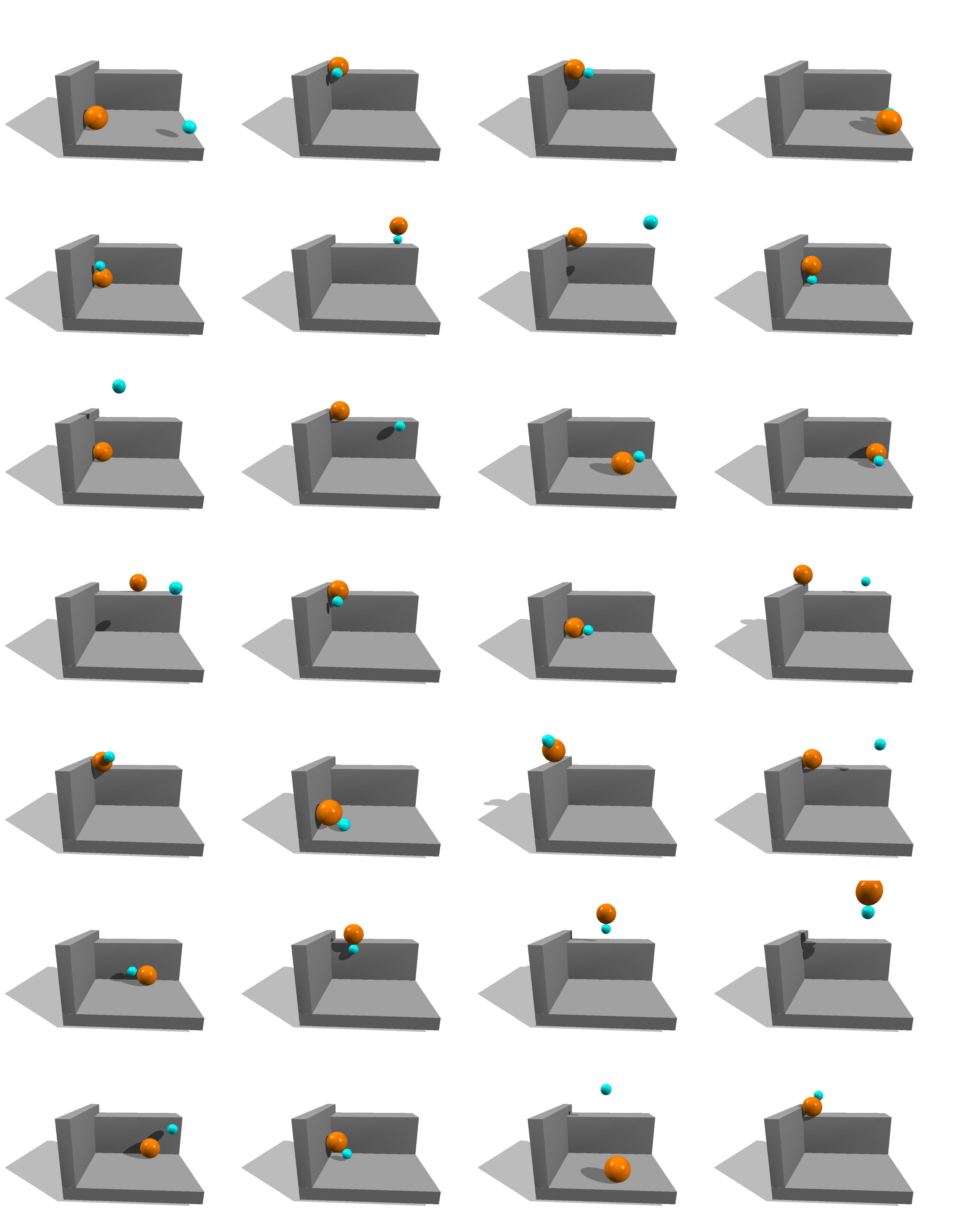
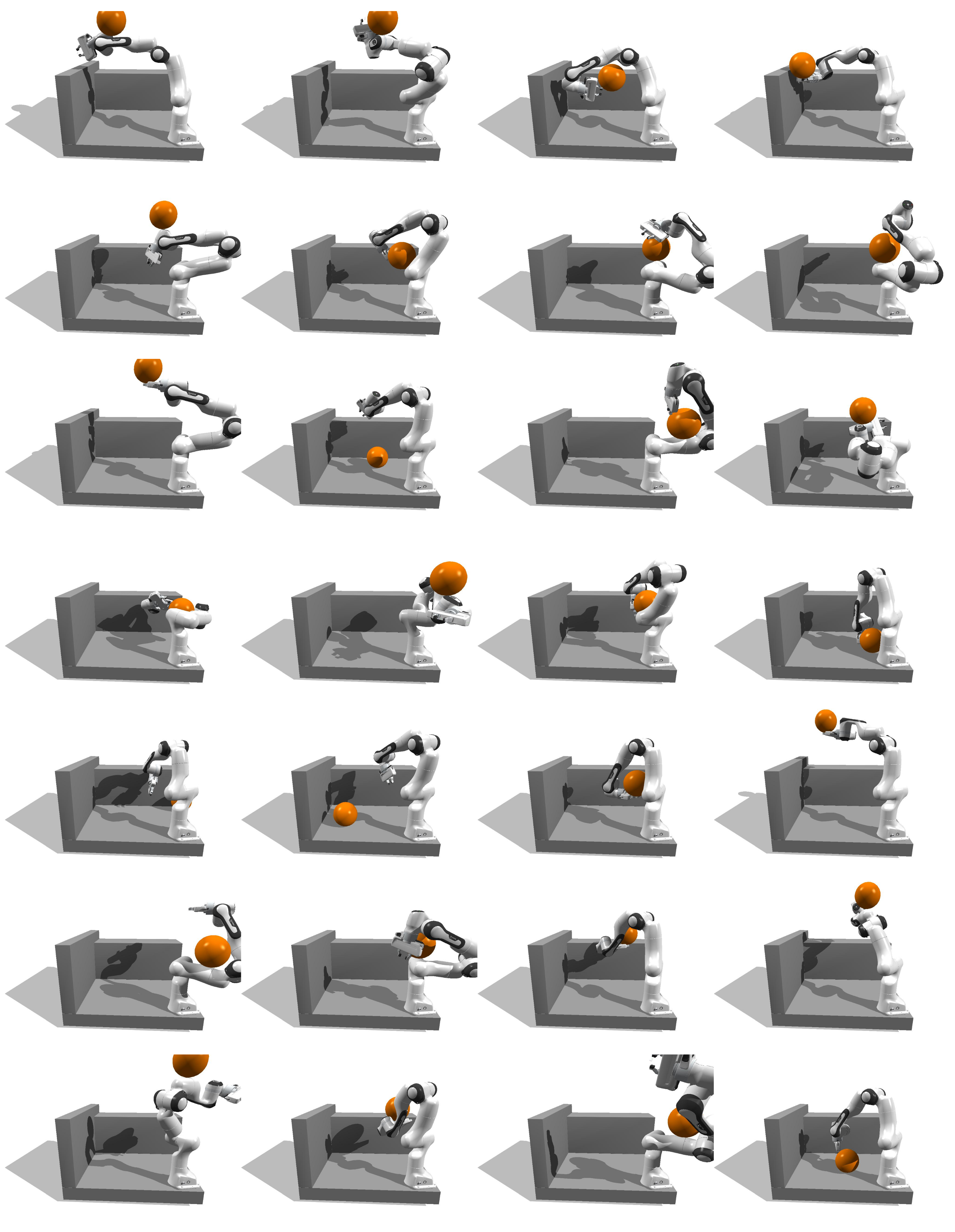
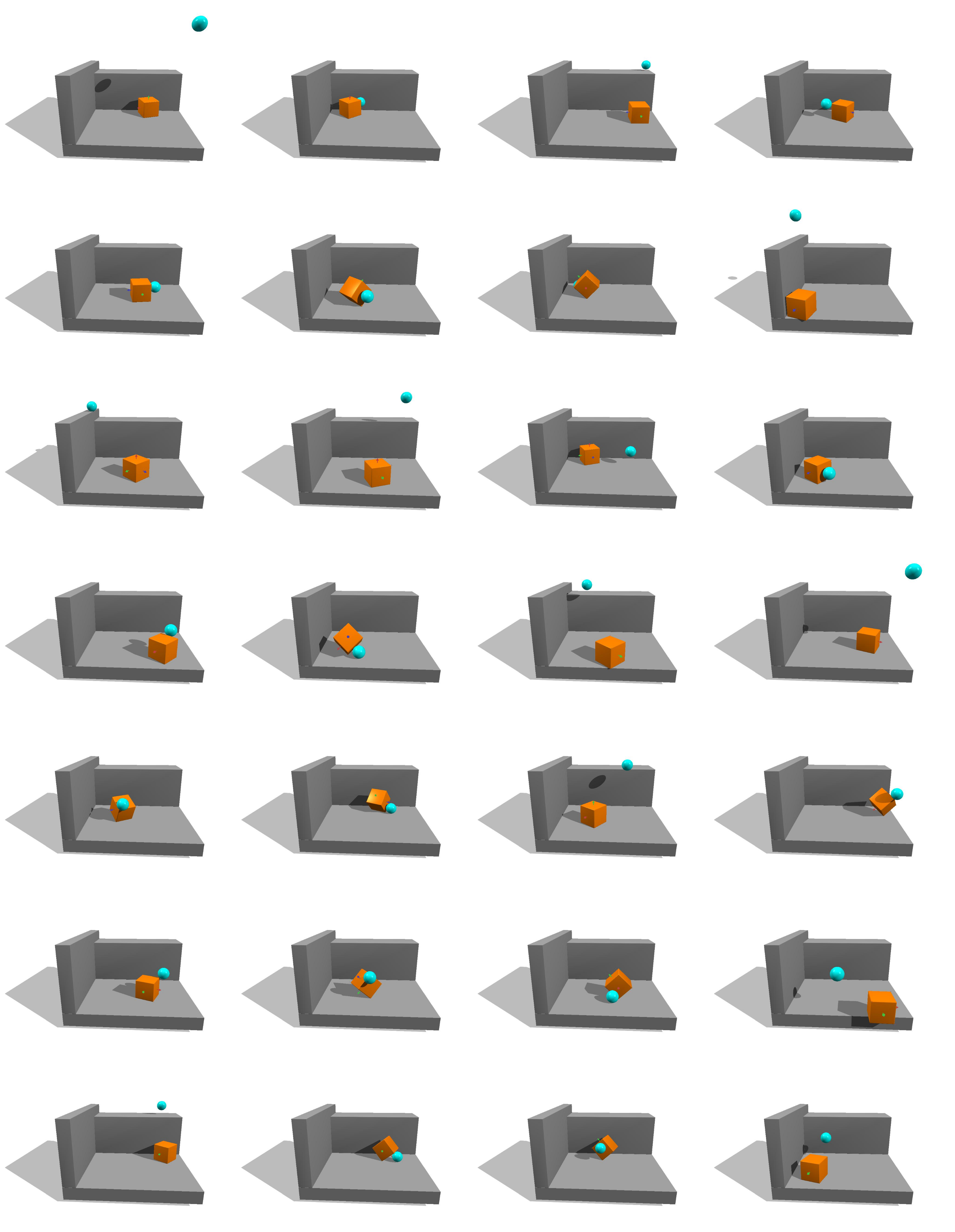
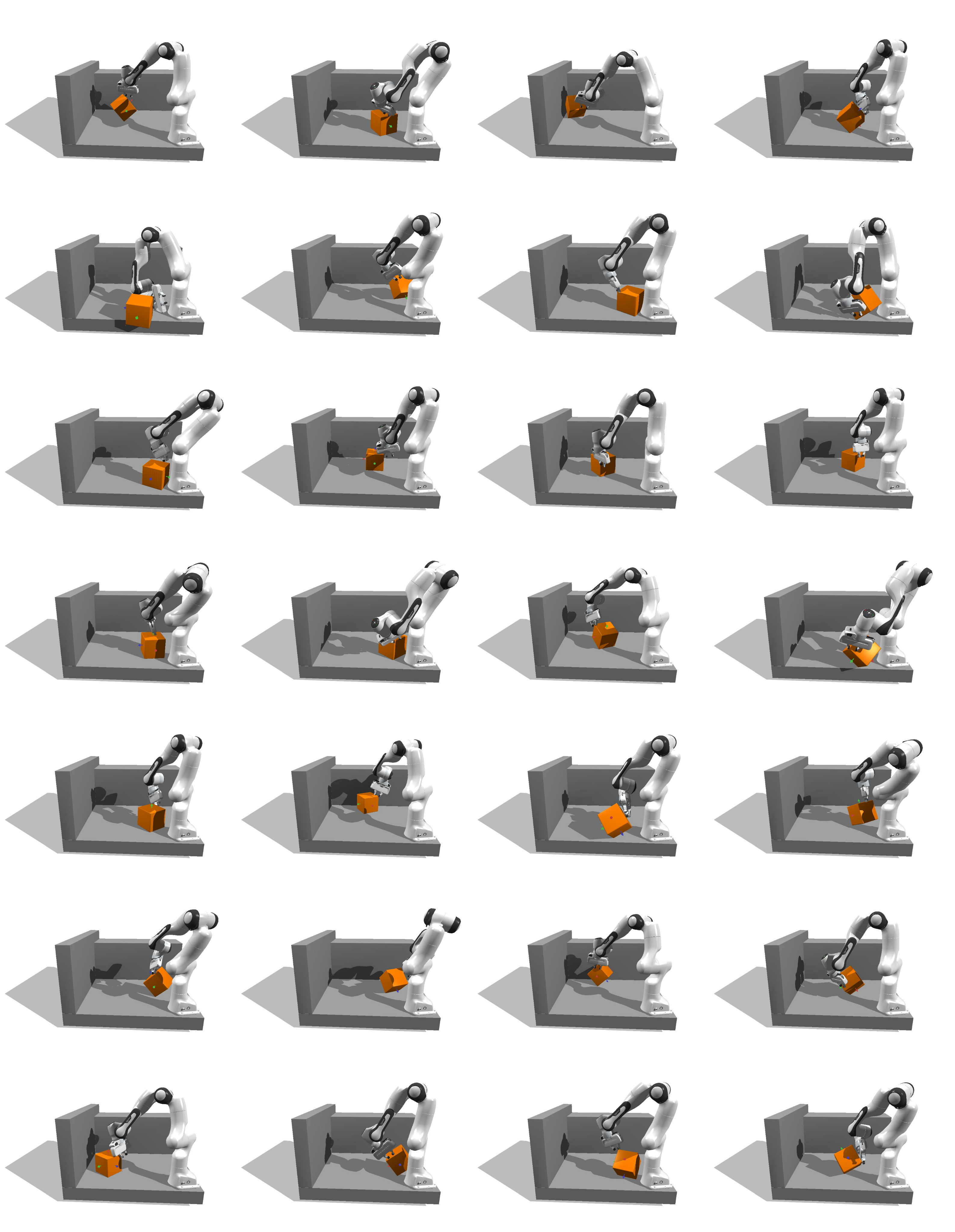
Overview
This edition covers the 25-page CoRL version, arXiv v3 dated 29 October 2026, including all six appendices and every sampled-state panel. The earlier preprint date remains in the publication metadata. Resources are linked from the author project page and code repository.
At a glance
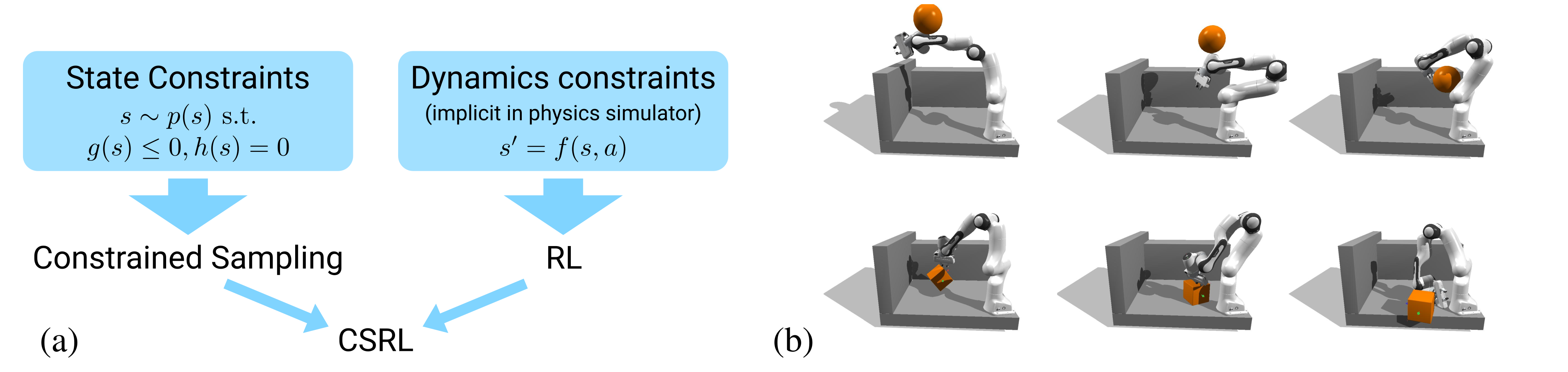
CSRL changes where manipulation training begins and which goals it attempts. A constrained solver samples collision-free, statically supportable contact configurations; a goal-conditioned RL policy then learns dynamic transitions between them. Nearest-sample projection of interpolated states and a short-to-long curriculum make distant goals easier to learn.
Across six simulated domains, constrained resets greatly improve exploration of whole-body and dexterous contacts. Benefits from interpolation, curriculum and HER depend on the domain. Hardware transfer is a qualitative ball-end-effector pushing demonstration with external state tracking, not a sensor-based general manipulation benchmark.
1 Introduction
Learning contact-rich behavior is difficult because random motion rarely reaches useful contacts. Planning complete trajectories through contact switches is also hard. The paper separates these problems: use physical constraints to generate diverse useful states, then let RL learn how to connect them.
“Universal” means goal-conditioned control within each fixed robot/object environment. The work does not demonstrate one policy across arbitrary new objects or robots. Static feasibility supplies a useful prior, but does not prove that every sampled start–goal pair is dynamically reachable.
2 Related Work
The method combines contact models from planning with reset and goal selection for reinforcement learning.
Model-based Manipulation Planning.
Explicit contact-mode planning and contact-implicit optimization exploit rigid-body structure but face nonsmooth, complementary contact dynamics. CSRL uses those constraints for isolated state generation rather than solving a complete trajectory, drawing on force-based manipulation planning.
Goal-conditioned RL & Universal Policies.
Universal value functions, goal relabeling, hierarchies and curricula usually assume useful goals are readily available. Here the difficult part is constructing feasible contact-rich starts and goals; the RL algorithm itself can be exchanged.
RL for Robot Manipulation.
Prior manipulation RL improves exploration, representations or trajectory-based supervision. CSRL instead changes the state distribution, including whole-arm and environmental contacts without reference motions. Experiments include both sparse rewards and a local progress-shaping variant.
Goal and Reset Distributions in RL.
Reverse curricula, Go-Explore and self-play expand reachable experience, while scene-drop and grasp samplers directly construct useful states. CSRL samples contact configurations globally under a model, avoiding commitment to a single grasp or pushing primitive.
3 Methods
The training recipe has three parts: define feasible contact states, generate a finite offline dataset, and use that dataset to schedule start–goal pairs for RL.
3.1 Problem Formulation
A constrained goal-conditioned MDP defines equality and inequality constraints over states, then optimizes expected discounted return over starts and goals. The mathematical objective specifies a uniform distribution on the feasible set.
The implemented sampler projects uniform box samples and rejects failed contact-mode solves. That procedure is not shown to sample the manifold uniformly; solver attraction regions and mode feasibility can bias coverage. Feasible reset states also need not contain every transient state visited during dynamic control.
Equations 1–3
| (1) |
| (2) | ||||
| (3) |
3.2 State Sampler
The constraint model assumes rigid shapes and goals that can be held in quasi-static equilibrium. The learned transitions may still be dynamic.
State Constraints.
Each potential shape pair has a binary contact indicator. All shapes must avoid penetration; active contacts must share a point of attack, apply a compressive normal force and remain inside a Coulomb friction cone. Unactuated objects must satisfy static force/torque balance.
The solver requires geometry, friction and Jacobians of distances/normals. These conditions describe model feasibility rather than guaranteed robustness to uncertain real contacts or actuator limits.
Equations 4–7
| (4) | ||||
| (5) | ||||
| (6) |
| (7) |
Non-linear Constrained Sampling.
For one manipulated free object, first choose one, two or three support contacts, then a support subset. Starting from a uniform configuration inside box bounds, an augmented-Lagrangian solver minimizes distance to that seed while satisfying contact and equilibrium constraints. Failed/local-optimum solves are discarded until the dataset is full.
This is simpler than the authors’ earlier MCMC/NLP sampler. The practical restriction to one object and at most three selected supports limits the claimed contact diversity. It samples endpoints, not paths or a certificate that transitions between them exist.
Equation 8
| (8) |

3.3 Additional Reset Strategies
Projected interpolation chooses a random start candidate and goal, interpolates their embeddings, and finds the nearest feasible dataset sample with a kd-tree. This preserves feasibility approximately through dataset membership; it is not a continuous constraint projection or a trajectory planner.
An optional curriculum increases the interpolation range from near-goal to full-range and proportionally lengthens episode truncation. Start–goal batches refresh every 5,000 training steps. The embedding combines weighted robot coordinates with object goal markers; sphere/cube weights are 0.5/0.2. HER can additionally relabel achieved goals.
Equations 9
| (9) |
4 Experiments
Default learning uses TD7 with a custom HER extension. Ablations change the state sampler, interpolation, curriculum and RL engine. Final tables report means and standard deviations over five runs; learning curves use standard errors.
4.1 Evaluation Domains
Double-Sphere uses a controllable sphere plus floor/walls; Panda-Sphere allows the sphere to rest against arm links. Sphere-Cube adds object orientation, and Panda-Cube uses gripper/finger contacts. Allegro-Cube requires in-hand position and orientation control; AllegroDown-Cube turns the hand over, making drops difficult to recover from.
Observations have 21, 42, 45, 66 and 96 dimensions, with 3-, 7- or 16-dimensional control. These are separate privileged-state environments with fixed objects. The paper does not specify a shared held-out start–goal test set or evaluation episode count in enough detail to establish identical coverage across different goal samplers.
| Double-Sphere | Panda-Sphere | ||||
| goals | starts | sparse | sparse | ||
| R | R | 0.521
0.394 |
0.596
0.325 |
0.051
0.073 |
0.058
0.076 |
| Ri | 0.769
0.032 |
0.772
0.036 |
0.073
0.075 |
0.035
0.069 | |
| Ric | 0.766
0.017 |
0.755
0.044 |
0.112
0.058 |
0.059
0.076 | |
| C | R | 0.867
0.018 |
0.685
0.373 |
0.005
0.004 |
0.007
0.002 |
| Ri | 0.877
0.010 |
0.697
0.386 |
0.154
0.175 |
0.012
0.013 | |
| Ric | 0.892
0.016 |
0.850
0.030 |
0.287
0.230 |
0.021
0.023 | |
| C | C | 0.963
0.011 |
0.953
0.004 |
0.527
0.255 |
0.472
0.450 |
| Ci | 0.972 0.007 | 0.783
0.430 |
0.630
0.415 |
0.701
0.466 | |
| Cic | 0.972 0.007 | 0.969 0.010 | 0.929 0.029 | 0.932 0.007 | |
| Double-Sphere | Panda-Sphere | ||||||
|---|---|---|---|---|---|---|---|
| goals | starts | TD7 | TD7 | TD3 | TD7 | TD7 | TD3 |
| C | C | 0.963
0.011 |
0.923
0.052 |
0.131
0.050 |
0.527
0.255 |
0.324
0.296 |
0.008
0.005 |
| Ci | 0.972
0.007 |
0.982 0.005 | 0.806
0.024 |
0.630
0.415 |
0.837
0.139 |
0.043
0.014 | |
| Cic | 0.972
0.007 |
0.983 0.005 | 0.800
0.006 |
0.929 0.029 | 0.814
0.104 |
0.066
0.009 | |
| goals | starts | Sphere-Cube | Panda-Cube | Allegro-Cube | AllegroDown-Cube |
|---|---|---|---|---|---|
| C | C | 0.878 0.032 | 0.949 0.009 | 0.954 0.011 | 0.903 0.025 |
| Ci | 0.912 0.048 | 0.966 0.005 | 0.957 0.006 | 0.901 0.023 | |
| Cic | 0.928 0.056 | 0.964 0.006 | 0.966 0.010 | 0.891 0.016 |
| goals | starts | Double-Sphere | Panda-Sphere |
|---|---|---|---|
| R | Rrev | 0.846 0.021 | 0.197 0.042 |
| C | Crev | 0.988 0.023 | 0.274 0.018 |
4.2 Comparison of Alternative State Samplers and Reset Strategies
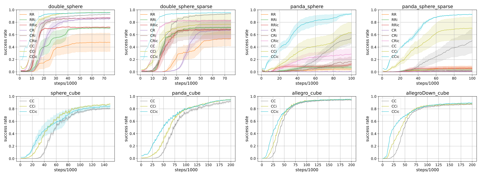
The random baseline drops uniformly initialized configurations in simulation until stable and rejects out-of-bounds states. With constrained goals, replacing those resets with constrained resets raises Panda-Sphere success from 0.005 to 0.527; adding interpolation/curriculum reaches 0.929. The corresponding sparse setting reaches 0.932. Double-Sphere reaches about 0.972.
The add-ons are not uniformly better. HER-free TD7 wins Double-Sphere in Table 2, while HER helps the full Panda curriculum. TD3 uses TD7 hyperparameters, so its weak results are not a fully tuned algorithm comparison. Table 2’s caption mentions TD3 HER although its columns are TD7-HER, TD7 and TD3-sb.
For cubes, full curriculum scores 0.928/0.964/0.966/0.891 across the four domains. Panda-Cube interpolation alone is slightly higher, and AllegroDown does best with plain constrained resets at 0.903. Constrained reverse curriculum scores 0.988 on Double-Sphere, above interpolation/curriculum’s 0.972, contradicting the claim that interpolation wins both sphere domains. Panda-Sphere strongly favors interpolation/curriculum over reverse curriculum’s 0.274.
Figure 3 retains all eight learning plots. Its caption says 80 environment samples per training step, whereas Appendix B specifies 2,000 samples per 20 updates, implying 100; the conversion is unresolved.
4.3 Discussion of Found Behaviors
Qualitative behaviors include balancing the sphere, scooping it onto arm links, rotating a cube onto an edge/corner, gripper squeezing and fingertip balancing. Some agile near-goal cube behavior misses the precision threshold. The inverted-hand domain trains useful behavior despite drop risk; it is not evidence of zero-shot transfer of the upright policy.
4.4 Real-World Transfer
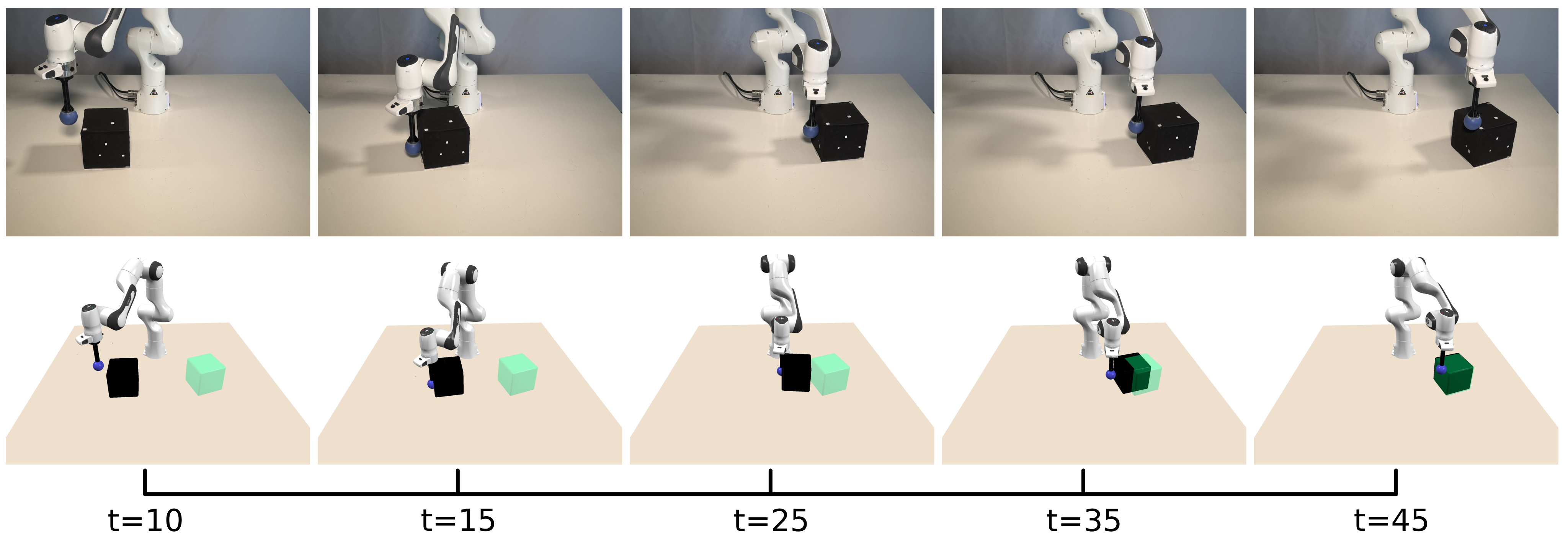
A Sphere-Cube policy controls a ball attached to a Panda arm through inverse kinematics. OptiTrack supplies cube state. Figure 4 pairs real and synchronized simulated views by action index; each blocking IK movement sets wall-clock duration.
This demonstrates basic pushing transfer with privileged tracking. The paper reports no hardware success rate, trial count or fixed real-time action frequency, and does not transfer its dexterous-hand policies to hardware.
5 Conclusion
Constraint-based reset design is the central contribution: useful contact states can improve RL exploration without solving every transition beforehand. Interpolation and a curriculum are inexpensive additions once the state dataset exists, but their gains vary across domains.
The explicit limitations are privileged state access, no sensor-based student policy, potential sim-to-real mismatch in contact/admittance observations, and expensive CPU constraint solving. Dedicated GPU solvers are future work. Single-object sampling, restricted support modes and unproven uniformity/reachability further delimit “universal” coverage.
Acknowledgments
Support includes BMFTR/Robotics Institute Germany, Amazon Fulfillment Technologies and Robotics, France 2030 (PEPR O2R, PR[AI]RIE-PSAI ANR-23-IACL-0008 and RODEO ANR-24-CE23-5886), and EU ARTIFACT 101165695 and AGIMUS 101070165. The authors state that their views do not necessarily represent the funders.
Appendix A Gym Environment Details
MuJoCo advances at 1 ms; actions arrive every 50 ms. PD motors track a quadratic reference overwritten by each action, with λ equal to two action intervals. Equation 10 makes the reference reach its initial position plus half the action after λ, while preserving reference position at the update.
Sphere goals use the object center; cube goals use its center and four corner markers. Success is the Euclidean marker-vector error below the domain threshold, not simply a position error in meters. Sparse reward gives one on success; local shaping rewards progress within ten thresholds. The claimed telescoping shaping bounds concern undiscounted episode sums.
Observations include joint positions/velocities, object velocity, control error, scene points and goal error. The control error exposes the reference state and indirectly contact forces. The prose says five Allegro fingertip points, but its 27 scene coordinates minus 15 object coordinates imply four 3D fingertip points; all original table dimensions remain.
At reset, arm/sphere reference positions match the configuration. Allegro resets instead back-project sampled contact forces to joint torques and offset the reference by torque divided by proportional gain, preloading a supporting grasp. This only approximately balances the cube in simulation. Table 4 preserves all training lengths, truncation times, thresholds, action scales, replay capacities and network widths.
Equations 10–11
| (10) |
| (11) |
| obs. dim | ||||||||||||
|---|---|---|---|---|---|---|---|---|---|---|---|---|
| Double-Sphere | 3 | 3 | 3 | 21 | 50k | 75k | 1. | 0.01 | 2. | 1M | 256 | 256 |
| Panda-Sphere | 7 | 12 | 3 | 42 | 50k | 100k | 2. | 0.01 | 5. | 2M | 512 | 256 |
| Sphere-Cube | 3 | 15 | 15 | 45 | 100k | 150k | 3. | 0.03 | 2. | 4M | 512 | 256 |
| Panda-Cube | 7 | 24 | 15 | 66 | 100k | 200k | 3. | 0.05 | 5. | 4M | 1024 | 512 |
| Allegro*-Cube | 16 | 27 | 15 | 96 | 100k | 200k | 3. | 0.02 | 2. | 5M | 1024 | 512 |
Equation
Appendix B TD7 & HER Extension Details
Following FastTD3-style parallel collection, each iteration adds 2,000 transitions and performs 20 TD7 updates with batch size 10,000. Learning rate is 10⁻³ except for Allegro. Shaped-return targets are clipped nonnegative as a stabilizing heuristic.
The custom HER buffer tracks previous transitions of each parallel episode. After at least three steps, the current next state becomes a relabeled goal for one earlier transition; goal-error observations, rewards and termination flags are all recomputed. This is the paper’s implementation-specific response to the cited wrapper behavior, not a statement about every current HER implementation.
Appendix C Statistics of Constraint Sampling
The offline datasets contain 20,000 states per sphere/Panda-cube domain and 50,000 per Allegro domain. Feasible-solve rates span 5.1%–48.8%; per-sample times span 38.7–576.8 ms, and total times span 0.22–4.80 hours.
Panda-Cube has the lowest feasible rate and most constraint queries; AllegroDown takes longest overall because it generates 50,000 states. Geometry-query cost and failed solves are material preprocessing costs, distinct from the RL training curves. Table 5 preserves all measurements.
| Double- Sphere | Panda- Sphere | Sphere- Cube | Panda- Cube | Allegro- Cube | AllegroDown- Cube | |
|---|---|---|---|---|---|---|
| number of samples | 20k | 20k | 20k | 20k | 50k | 50k |
| feasibility rate | 0.356 | 0.116 | 0.214 | 0.051 | 0.488 | 0.121 |
| queries/sample | 578.3 | 2934.9 | 876.0 | 6681.5 | 394.3 | 2645.7 |
| time/sample [msec] | 38.7 | 221.3 | 44.6 | 576.8 | 77.6 | 345.2 |
| total time [h] | 0.22 | 1.23 | 0.24 | 3.20 | 1.08 | 4.80 |
Appendix D Real World Transfer Setup
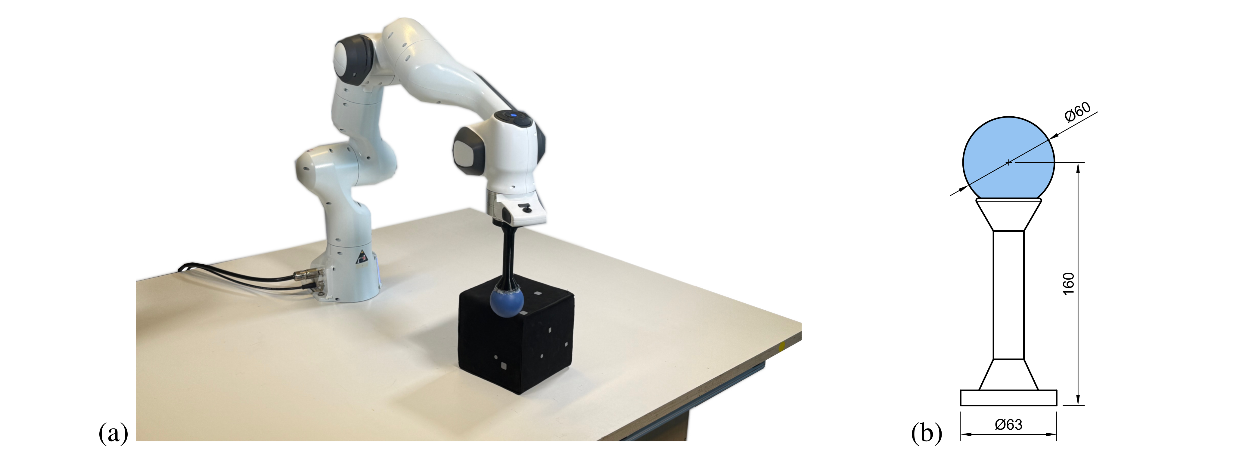
The physical Panda carries a custom ball, positioned 16 cm from the flange. Twelve OptiTrack Flex13 cameras track the cube. Figure 5 retains the setup photograph and exact dimensional drawing. The prose specifies a 3 cm ball radius, but the drawing labels its diameter 80 mm, implying a 4 cm radius; that mismatch is unresolved.
Appendix E Comparison to Behavior Cloning from Diverse Trajectory Data
The appendix preserves a negative result from arXiv v1: generating diverse open-loop trajectories was costly, and adding a BC loss contributed less than using their states as resets. The current version reports the method and qualitative interpretation but refers to v1 for the numerical results; later RL hyperparameter improvements prevent direct score comparison.
E.1 Zero-Order Optimization of Open-Loop Trajectories
For sampled starts/goals, CMA-ES searches a low-dimensional B-spline action sequence under deterministic simulated dynamics. The terminal objective compares weighted object position, robot configuration, their velocities and contact-proximity features. Nearby-support features supply a useful search signal before object motion occurs.
There is no explicit control-effort cost; smoothness comes from the spline parameterization. Only trajectories meeting the terminal threshold enter the dataset. This is a black-box optimizer over a known simulator, not a demonstration that model-based trajectory generation is impossible.
Equations 12–13
| (12) |
| (13) |
E.2 Behavior Cloning from Trajectory Data
The proposed TD7+BC extension follows TD3+BC. Aligned quadratic spline segments are converted into the same 20 Hz action parameterization, producing state–goal–action examples that reproduce the deterministic simulated path.
Equation 14 prints a maximization with a plus sign before λ times squared imitation error. With positive λ that would reward disagreement; the sign convention is not clarified, so the original formula is retained. The experiment also changes reset states to trajectory states, making it essential to separate the BC-loss effect from the reset-distribution effect.
Equations 14–15
| (14) |
| (15) |
E.3 Results: What is the role of BC in effective universal RL?
The authors report that trajectory-derived resets substantially improve learning while the imitation term has little additional impact. Reactive learned rollouts can correct disturbances that the open-loop spline plans do not handle. This is a negative result for the tested data/training regime, not a general rejection of behavior cloning; current-version numerical comparisons are absent.
Appendix F Random Constrained Samples from our Domains
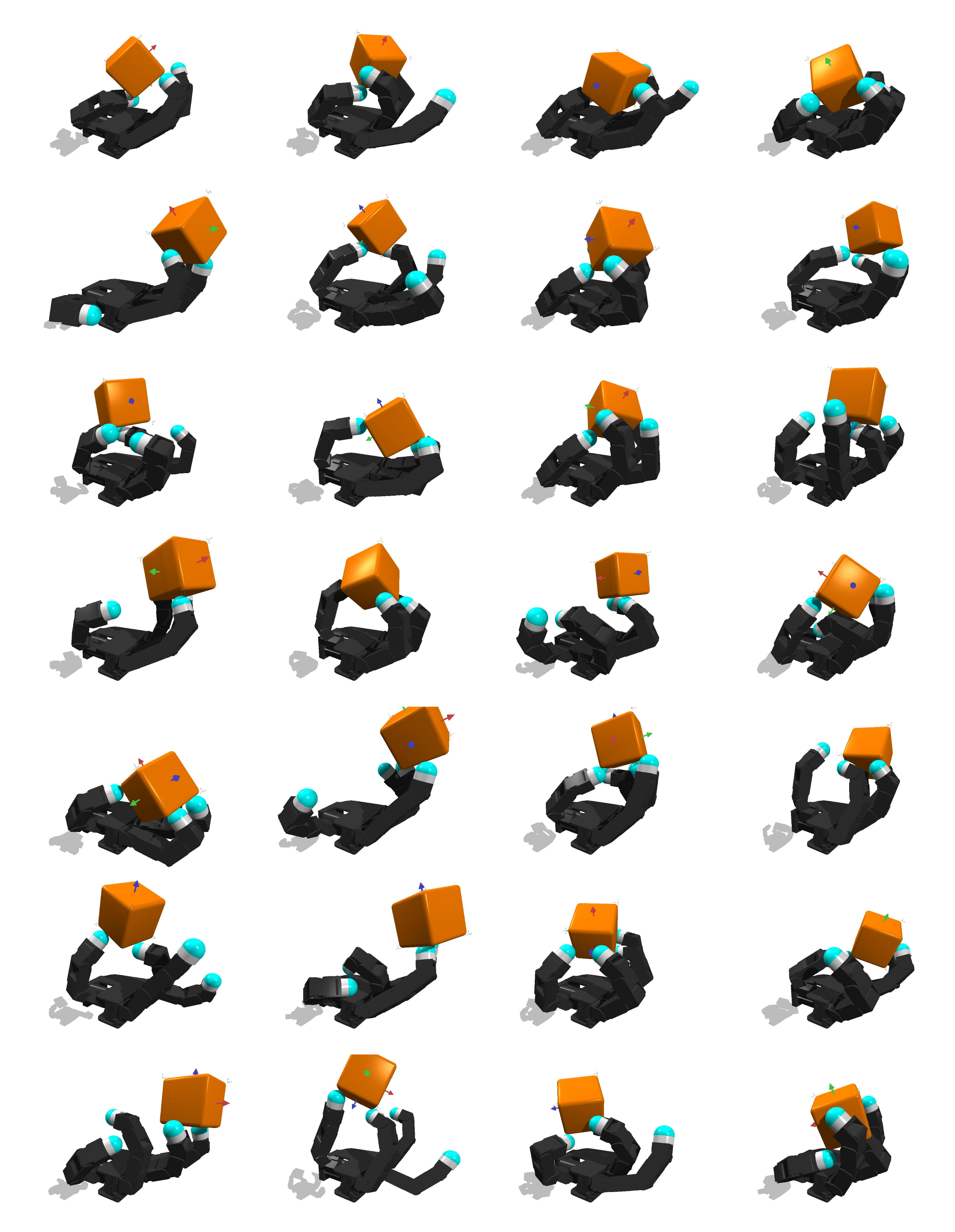
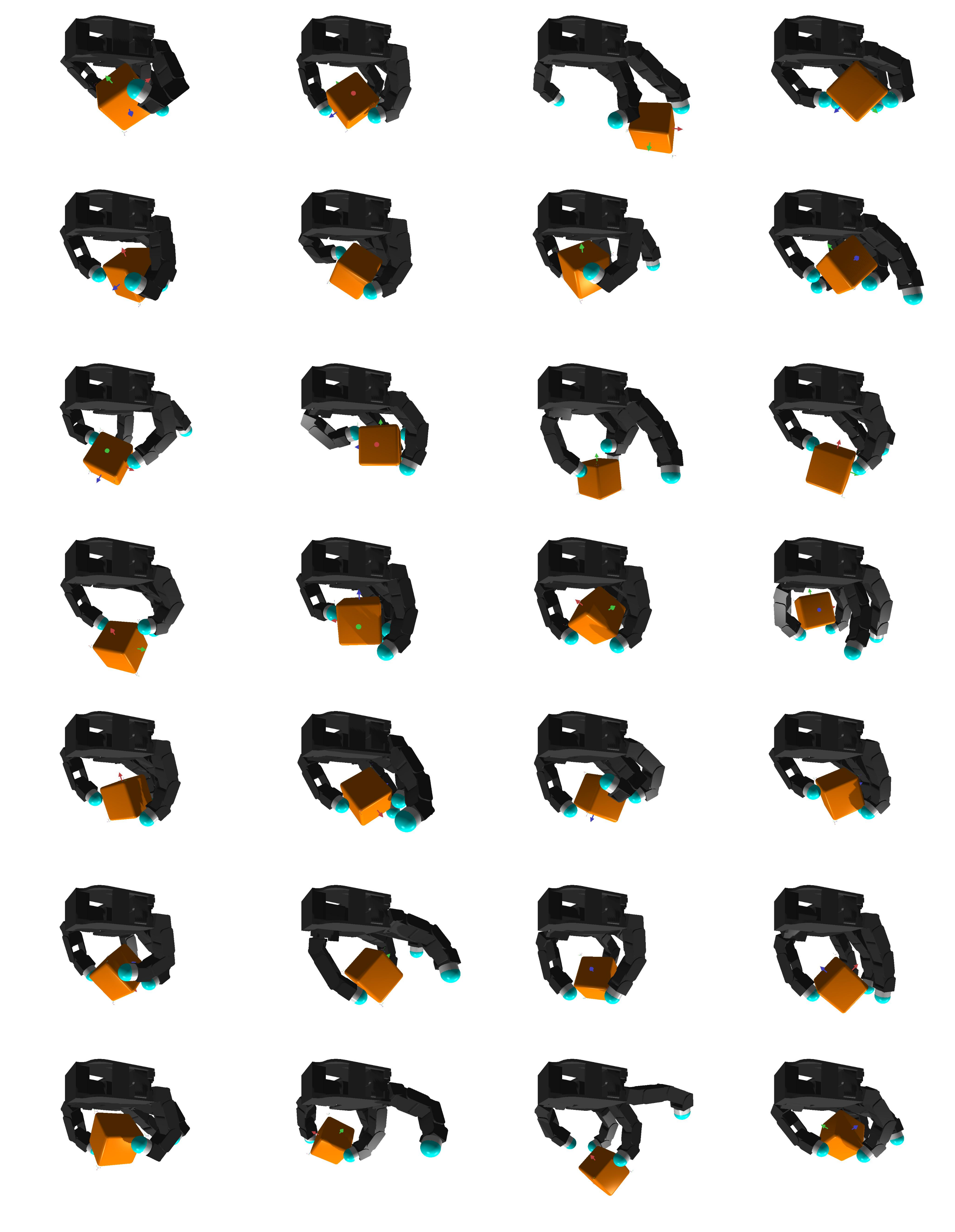
Figures 6–11 preserve all six 28-panel sample grids, totaling 168 configurations. The introduction’s “four domains” is stale wording. Figures 10 and 11 retain the original erroneous “panda cube” captions; their images depict Allegro-Cube and AllegroDown-Cube, respectively. Samples illustrate coverage, not a measured uniform distribution or guaranteed executable transitions.