At a glance
Use a differentiable analytic IK map as the optimizer’s coordinate system. End-effector constraints become linear, while joint limits, collision avoidance and costs are evaluated through the map. This improves feasibility in many tested cases, but does not guarantee faster solves or better objective values.
The framework combines analytic inverse kinematics with general nonlinear optimization. Experiments compare joint-space and analytic-coordinate formulations using interior-point, augmented-Lagrangian and sequential-quadratic solvers, plus sampling and a mixed-integer baseline. All reported robot experiments are simulations; the principal benefit is feasibility under difficult constraints.
I Introduction
Analytic IK is fast for supported kinematic structures but handles general constraints awkwardly. Joint-space optimization handles redundancy, collision avoidance and whole-body goals, yet couples them to a difficult nonlinear end-effector equality. The paper changes coordinates so that the analytic solution enforces that kinematic relationship.
This edition covers all 19 pages of arXiv v1, dated 4 February 2026, with all four authors verified. Thomas Cohn and Lihan Tang contributed equally. Every figure panel, table, displayed equation and appendix is retained.
I-A Our Contributions
Optimize pose and self-motion parameters, then differentiate through analytic IK to recover joint configurations, building on prior constrained bimanual planning. The transformation trades a simple end-effector constraint for more complicated costs, joint-limit constraints and explicit reachability checks.
Additional contributions repair PR2/idealized-Hubo mappings, strengthen the Global-IK baseline with automatic free-space decomposition and a joint-centering proxy, and express static support stability using inequalities. The experiments support a feasibility advantage, rather than a general theorem of easier or globally optimal optimization.
II Related Work
The review spans special-geometry analytic solutions, symbolic/code-generated IK, geometric subproblem decomposition, polynomial elimination, generic nonlinear and convex-relaxation methods, numerical iterative IK, and learned mappings. Existing hybrid methods often specialize to one robot or solver; this framework targets differentiable analytic maps and generic constrained optimizers.
Specialized numerical and learned IK methods are discussed but not directly benchmarked. Their absence limits claims about the strongest available solver for a particular application.
III Background
Joint configurations live on a torus, subject to limits; forward kinematics maps them into rigid poses. The notation distinguishes frame-relative position, orientation and homogeneous transforms. Euler angles are used to avoid adding unit-quaternion or rotation-matrix equality constraints to the new formulation.
III-A The Topology of Robot Kinematics
Redundancy permits motion along an end-effector-preserving manifold. Kinematic singularities lose instantaneous task-space directions; representational singularities can also arise from the chosen coordinates. The argument relies on regular local mappings, not a single globally nonsingular coordinate chart.
III-B A Look Inside Analytic IK Functions
The analytic map takes target pose, continuous redundancy parameters and a discrete branch index, and returns joint angles. Joint limits usually require separate checks, and unreachable inputs trigger domain violations such as an arccos argument outside [−1,1]. Both kinematic and coordinate singularities complicate numerical differentiation.
Equation 1
| (1) |
IV Methodology
Instrument each domain-limited operation with an unclipped probing function. For arccos(f), constraints 1−f≥0 and 1+f≥0 certify its valid input range. Clip the value used by IK to avoid undefined evaluations, while retaining the original probe gradients to guide the optimizer toward reachability.
Equations 2–3b
| (2) |

Original selectable MathML (source has misplaced frame superscripts)
| (3a) | ||||
| (3b) | ||||
IV-A Reformulation of Optimization IK with Analytic IK
The old and new formulations retain the same physical objectives and additional constraints, but expose different decision variables and numerical geometry.
IV-A 1 An Existing Formulation
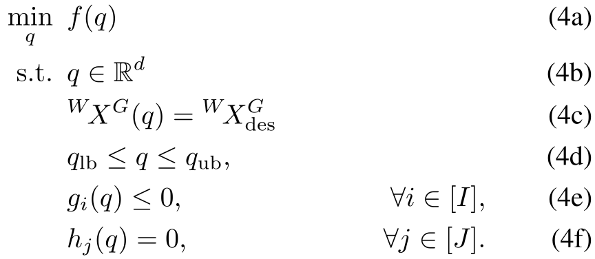
Equation 4 optimizes joint angles with a nonlinear pose equality, box joint limits and arbitrary extra inequality/equality constraints. Joint centering is a typical objective; collisions and stability supply harder constraints.
Equations 4a) (4b) (4c) (4d) (4e) (4f–4f
Original selectable MathML (source has misplaced frame superscripts)
| (4a) | |||||
| (4b) | |||||
| (4c) | |||||
| (4d) | |||||
| (4e) | |||||
| (4f) | |||||
IV-A 2 Reformulation
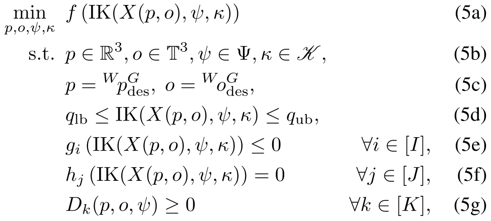
Equation 5 replaces joint variables with end-effector position/orientation, continuous redundancy and an IK branch. Pose matching is now linear; costs and joint constraints are composed with IK, and reachability probes are added. In practice, fix one discrete branch for each solve rather than solve the full mixed-integer problem.
This can make the IK equality extremely accurate, but other nonlinear equalities remain. A fixed branch can exclude every feasible solution or the best objective value. Enumerating branches is possible but not the default comparison.
Equations 5a) (5b) (5c) (5d) (5e) (5f) (5g–5g
Original selectable MathML (source has misplaced frame superscripts)
| (5a) | |||||
| (5b) | |||||
| (5c) | |||||
| (5d) | |||||
| (5e) | |||||
| (5f) | |||||
| (5g) | |||||
IV-A 3 Some Immediate Generalizations
Partial pose targets, bounded pose error and soft target costs follow by freeing appropriate pose variables. Multiple chains use separate analytic maps coupled through shared base/torso variables, as in the PR2 and Hubo examples. These generalizations still require valid differentiable mappings for each chain.
IV-A 4 Handling Domain Limitations of the IK Function
Clipping allows intermediate infeasible iterates, while unclipped probes supply recovery gradients. Inputs are clipped slightly inside their domain to keep derivatives finite. “Nearest valid solution” is informal here, not a proved least-squares projection. Humanoid experiments instead need solver-specific hard-domain handling and logarithmic barriers.
V Experiments
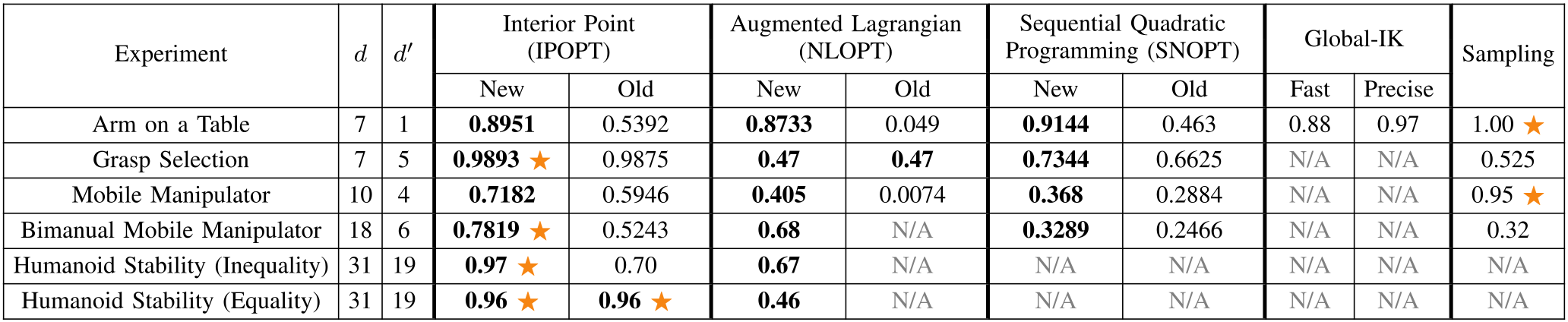
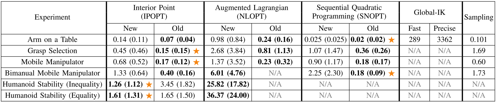
Compare IPOPT, SNOPT and augmented Lagrangian through NLopt. Sampling searches redundancy and branch choices; Global-IK is tractable only for the first task. Tables I–III preserve success, successful-solve cost and runtime separately.
Global-IK success rejects collisions but does not demand exact target pose, because its rotation relaxation introduces pose error. Cost comparisons condition on different successful subsets. Runtime comparisons also mix mostly C++ old-formulation code with substantial Python work in the new formulation.
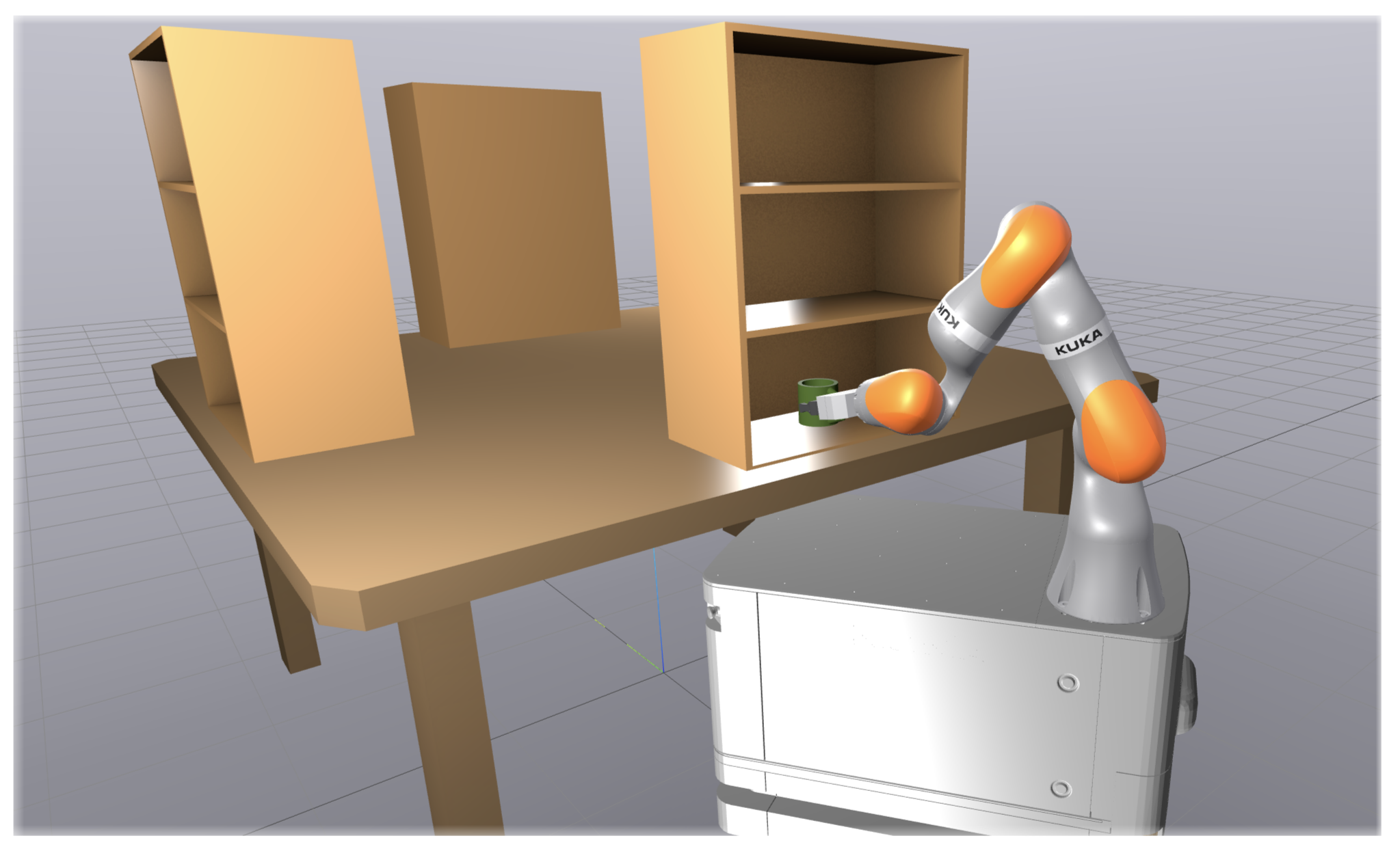
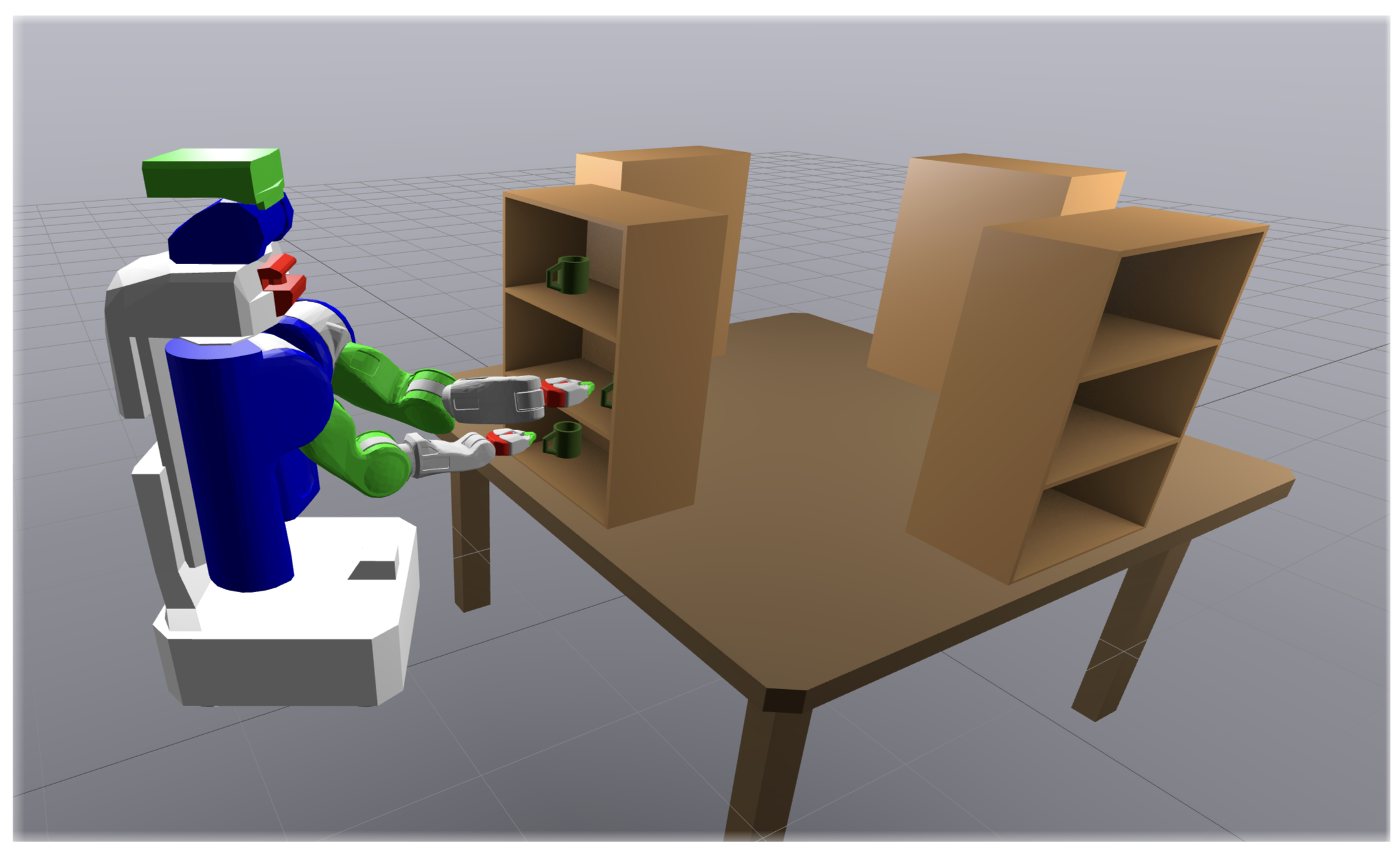
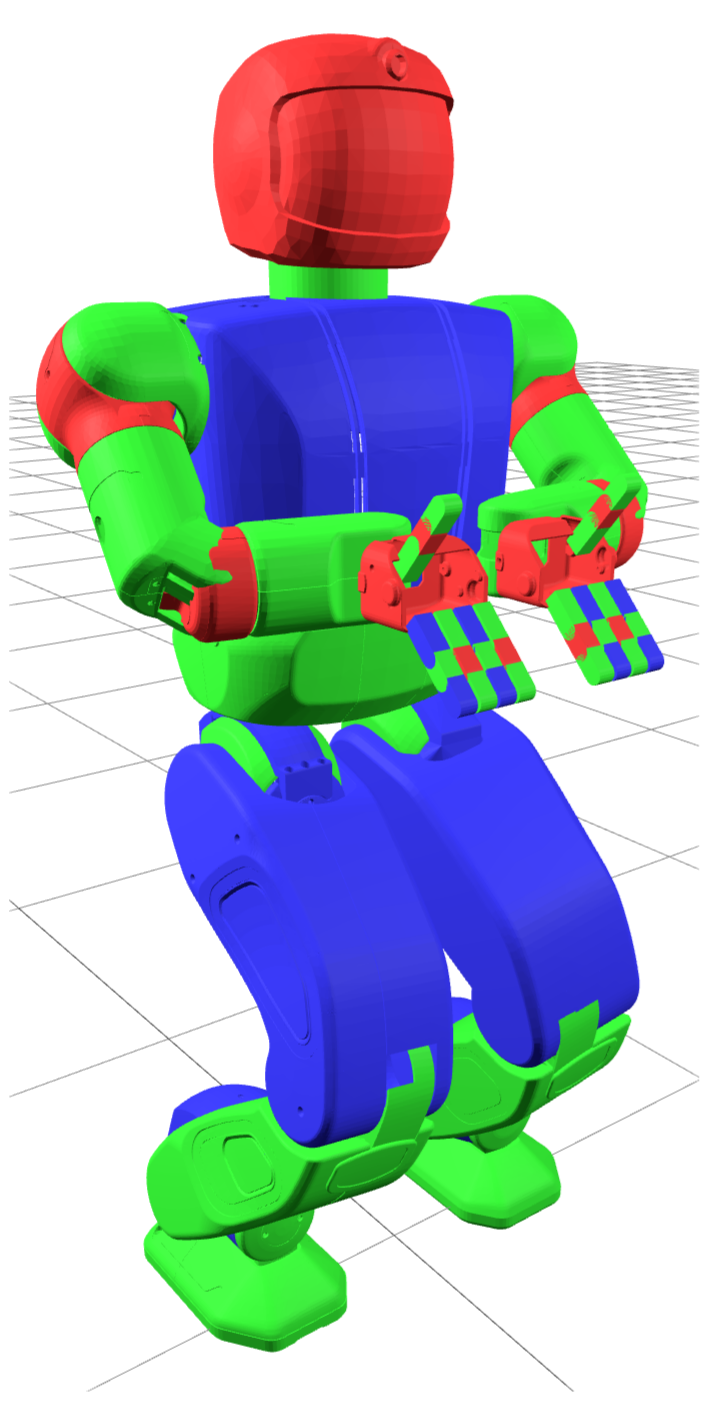
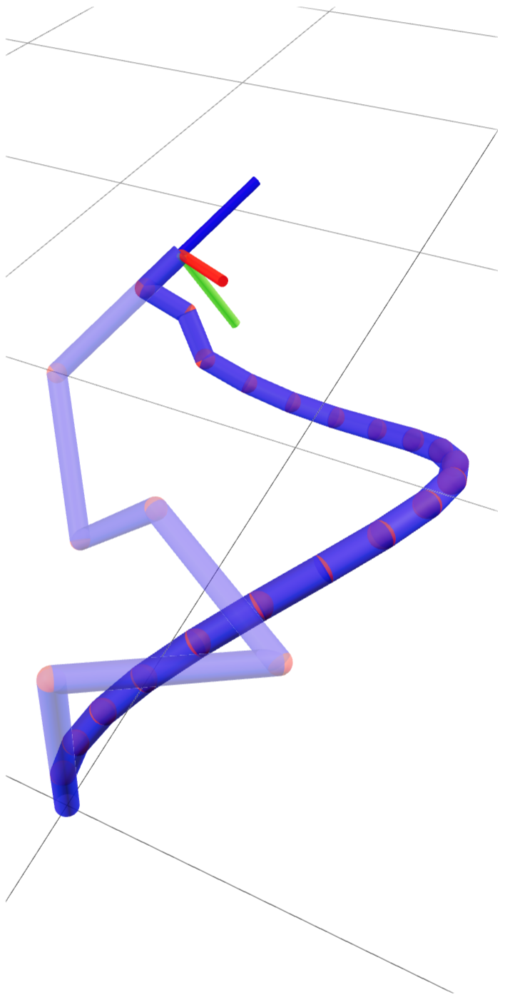
Original selectable source
| Experiment | Interior Point (IPOPT) | Augmented Lagrangian (NLOPT) | Sequential Quadratic Programming (SNOPT) | Global-IK | Sampling | ||||||
|---|---|---|---|---|---|---|---|---|---|---|---|
| New | Old | New | Old | New | Old | Fast | Precise | ||||
| Arm on a Table | 7 | 1 | 0.8951 | 0.5392 | 0.8733 | 0.049 | 0.9144 | 0.463 | 0.88 | 0.97 | 1.00 |
| Grasp Selection | 7 | 5 | 0.9893 | 0.9875 | 0.47 | 0.47 | 0.7344 | 0.6625 | N/A | N/A | 0.525 |
| Mobile Manipulator | 10 | 4 | 0.7182 | 0.5946 | 0.405 | 0.0074 | 0.368 | 0.2884 | N/A | N/A | 0.95 |
| Bimanual Mobile Manipulator | 18 | 6 | 0.7819 | 0.5243 | 0.68 | N/A | 0.3289 | 0.2466 | N/A | N/A | 0.32 |
| Humanoid Stability (Inequality) | 31 | 19 | 0.97 | 0.70 | 0.67 | N/A | N/A | N/A | N/A | N/A | N/A |
| Humanoid Stability (Equality) | 31 | 19 | 0.96 | 0.96 | 0.46 | N/A | N/A | N/A | N/A | N/A | N/A |
V-A Arm on a Table
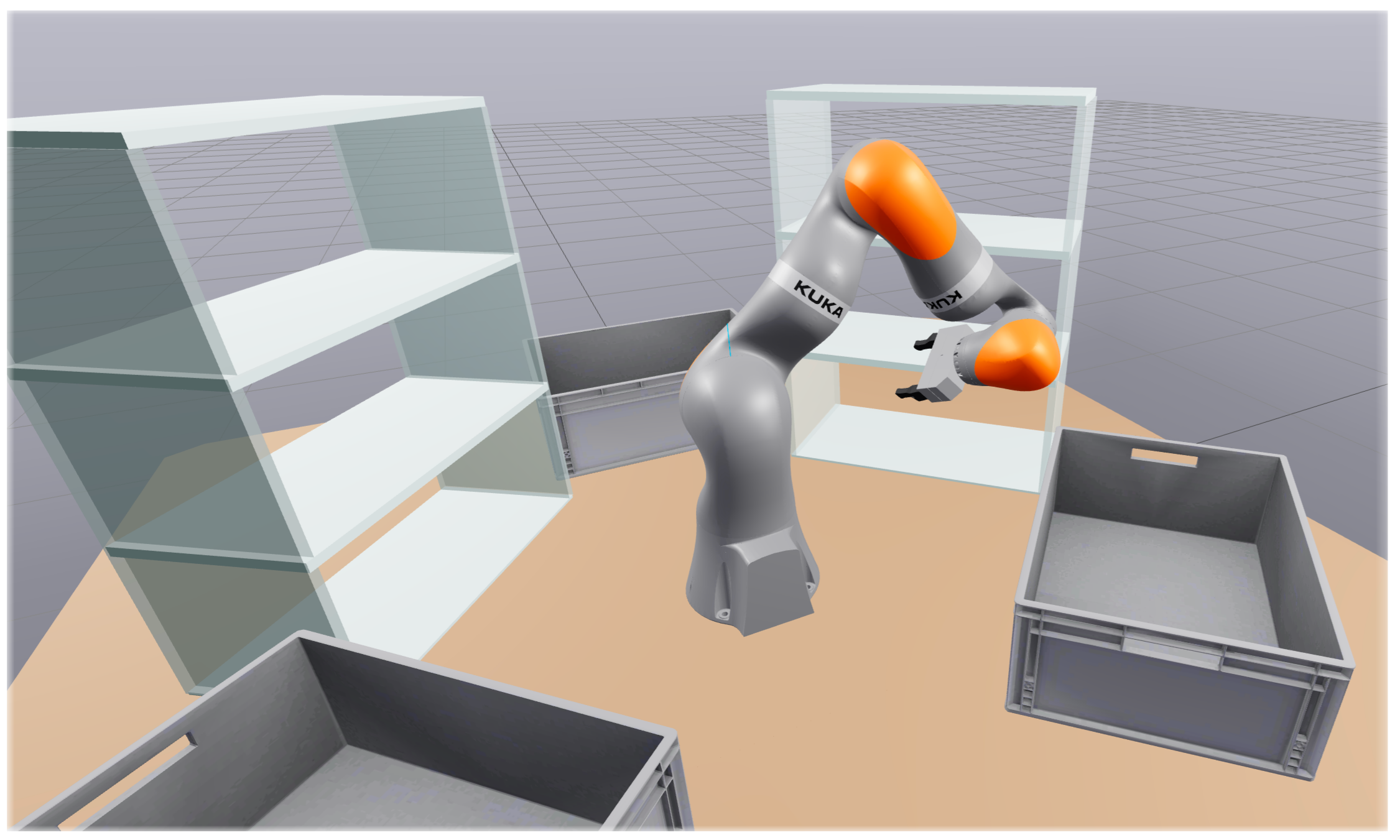
A seven-joint iiwa reaches 100 feasible target poses from 100 matched starts each, with collision avoidance and joint centering. New/old success is 89.51%/53.92% for IPOPT, 87.33%/4.9% for NLopt and 91.44%/46.3% for SNOPT. Sampling all branches reaches 100% in this one-dimensional redundancy space.
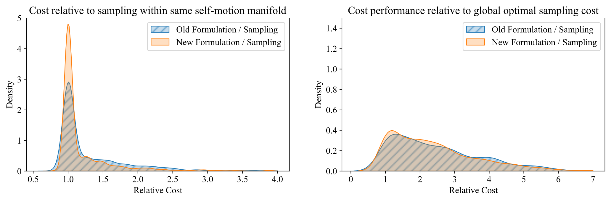
Dense sampling estimates that a random target/branch pair is feasible only 94% of the time, bounding this fixed-branch protocol. Figure 2 shows that much of the cost disadvantage comes from branch restriction; its sampled “global optimum” is a dense-search reference, not a formal global certificate. Global-IK has 88%/97% success for fast/precise settings, but average pose error about 8/1 cm and runtimes 289/3362 seconds.
V-B Grasp Selection IK
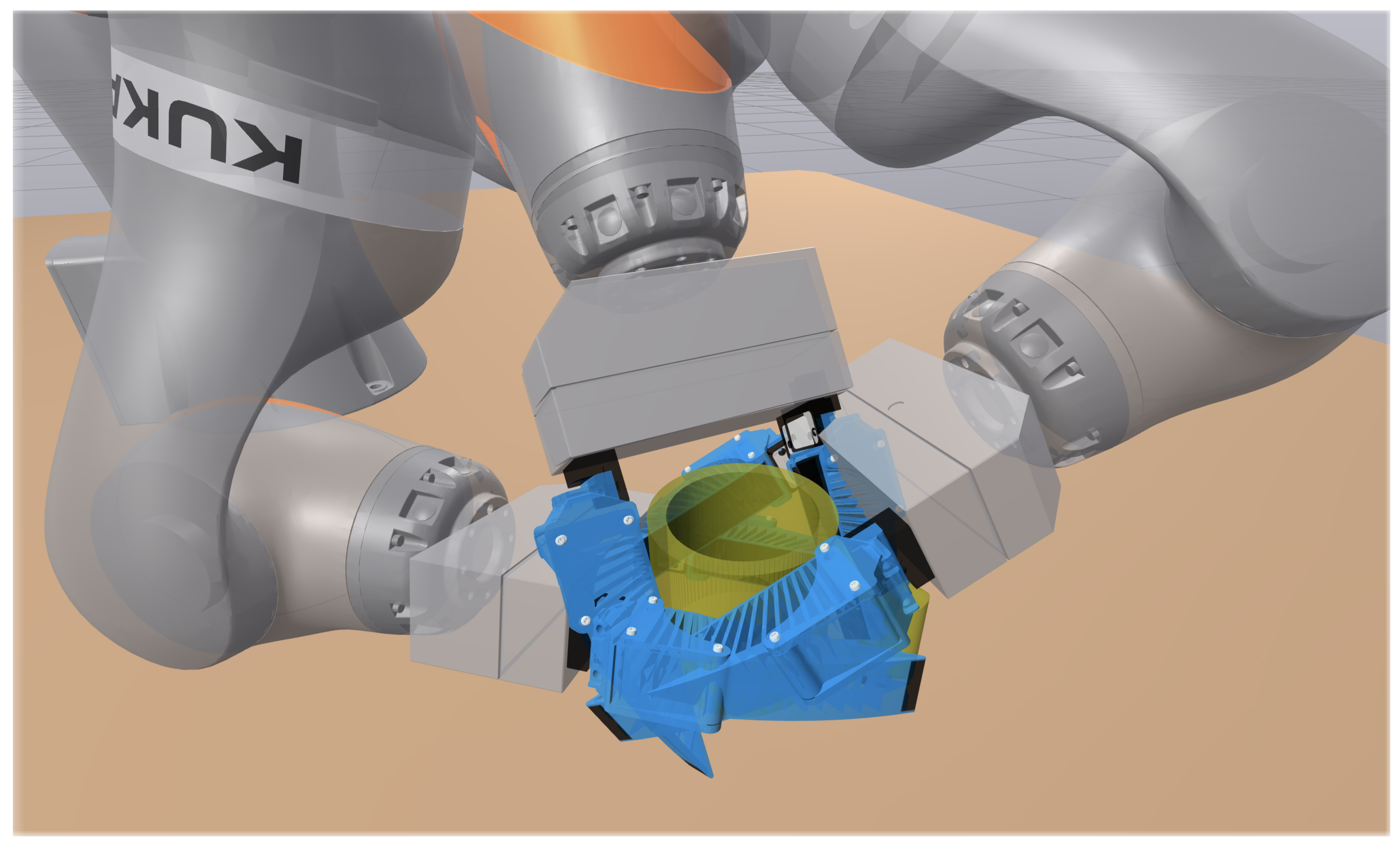
Place a point between the fingers on a mug’s central axis while leaving orientation free; collision constraints select plausible grasps. Forty targets and forty starts yield 1,600 solves. IPOPT new/old success is 98.93%/98.75%, but mean successful cost is 9.22/5.83 and runtime 0.45/0.15 seconds.
Sampling 8,192 points succeeds only 52.5% in five dimensions. Removing the objective yields reported 100% feasibility for both formulations. Similar best costs over forty starts suggest comparable accessible minima, without proving global optimality.

Original selectable source
| Experiment | Interior Point (IPOPT) | Augmented Lagrangian (NLOPT) | Sequential Quadratic Programming (SNOPT) | Global-IK | Sampling | ||||
|---|---|---|---|---|---|---|---|---|---|
| New | Old | New | Old | New | Old | Fast | Precise | ||
| Arm on a Table | 14.1 | 14.6 | 14.3 | 11.3 | 14.2 | 15.0 | 5.5 | 5.8 | 6.1 |
| Grasp Selection | 9.22 | 5.83 | 10.9 | 3.6 | 10.9 | 14.0 | N/A | N/A | 7.44 |
| Mobile Manipulator | 8.46 | 7.28 | 8.62 | 3.44 | 10.8 | 6.81 | N/A | N/A | 14.58 |
| Bimanual Mobile Manipulator | 35.2 | 25.5 | 30.6 | N/A | 37.7 | 29.8 | N/A | N/A | 43.8 |
Original selectable source
| Experiment | Interior Point (IPOPT) | Augmented Lagrangian (NLOPT) | Sequential Quadratic Programming (SNOPT) | Global-IK | Sampling | ||||
|---|---|---|---|---|---|---|---|---|---|
| New | Old | New | Old | New | Old | Fast | Precise | ||
| Arm on a Table | 0.14 (0.11) | 0.07 (0.04) | 0.98 (0.84) | 0.24 (0.16) | 0.025 (0.025) | 0.02 (0.02) | 289 | 3362 | 0.101 |
| Grasp Selection | 0.45 (0.46) | 0.15 (0.15) | 2.68 (3.84) | 0.81 (1.13) | 1.07 (1.47) | 0.36 (0.26) | N/A | N/A | 1.69 |
| Mobile Manipulator | 0.68 (0.52) | 0.17 (0.12) | 1.37 (3.52) | 0.23 (0.32) | 0.90 (1.17) | 0.18 (0.17) | N/A | N/A | 0.60 |
| Bimanual Mobile Manipulator | 1.33 (0.64) | 0.40 (0.16) | 6.01 (4.76) | N/A | 2.25 (2.30) | 0.18 (0.09) | N/A | N/A | 1.73 |
| Humanoid Stability (Inequality) | 1.26 (1.12) | 3.45 (1.82) | 25.82 (17.82) | N/A | N/A | N/A | N/A | N/A | N/A |
| Humanoid Stability (Equality) | 1.61 (1.31) | 1.65 (1.50) | 36.37 (24.00) | N/A | N/A | N/A | N/A | N/A | N/A |
V-C A Basic Mobile Manipulator
A mobile iiwa adds planar base pose, giving four redundancy dimensions. Use 100 targets and 100 collision-free starts each. IPOPT new/old success is 71.82%/59.46%; its new successful cost and runtime are worse. Removing the objective raises reported feasibility to 98%/95%.
Reachability probes help move the base until the arm can reach. Sampling succeeds 95% but has a higher mean cost. This task’s collision-free initialization is more favorable than the fixed-arm protocol, so cross-task differences are not solely caused by redundancy.
V-D A Bimanual Mobile Manipulator
The PR2 has two seven-joint arms coupled by planar base pose and torso lift. Forty targets and forty collision-free starts produce 1,600 trials. IPOPT new/old success rises from 52.43% to 78.19%; the new mean cost is 35.2 versus 25.5 and runtime 1.33 versus 0.40 seconds.
Base orientation can trap both formulations in crossed-arm infeasibility. The old NLopt formulation finds no feasible solutions. Sampling succeeds only 32% despite restricting the base near the targets; the six-dimensional feasible set is narrow.
V-E Humanoid Stability
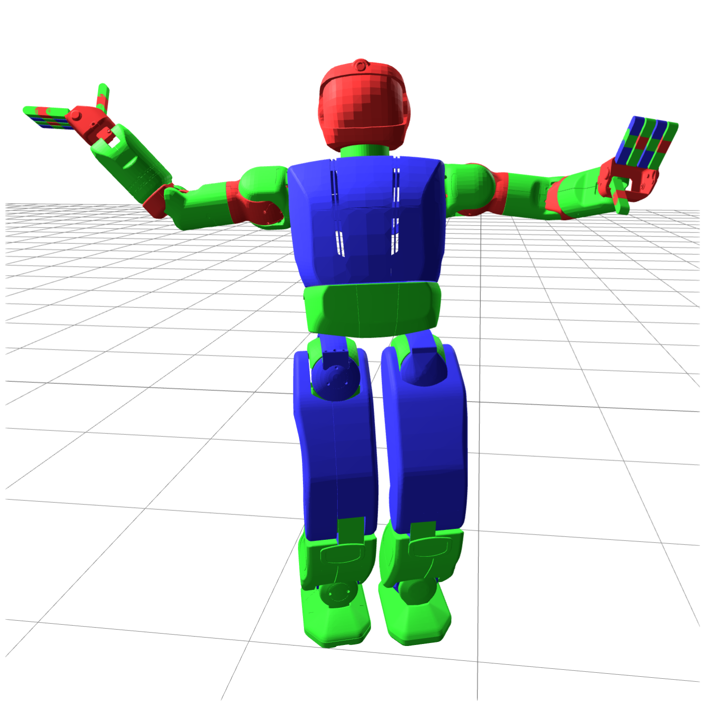
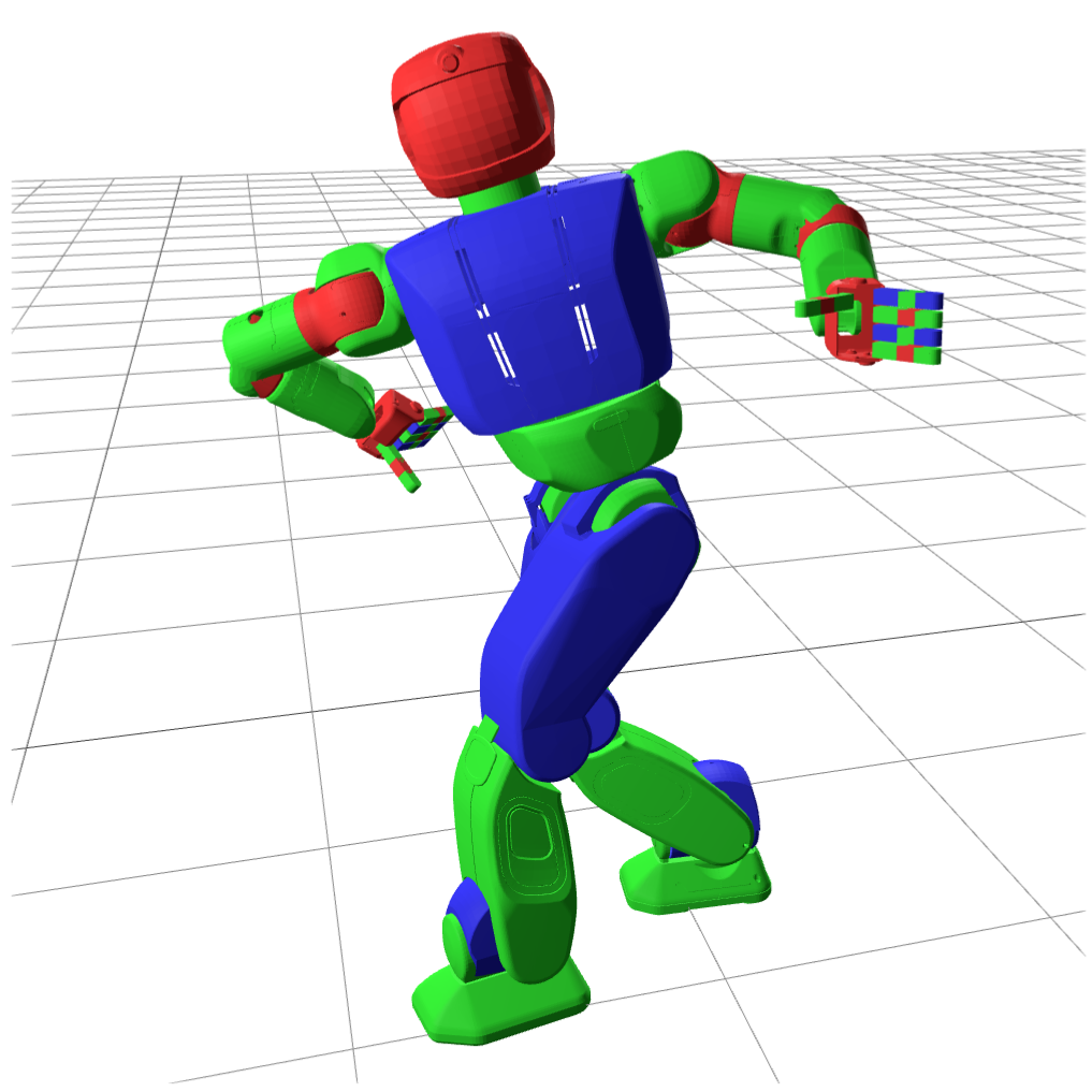
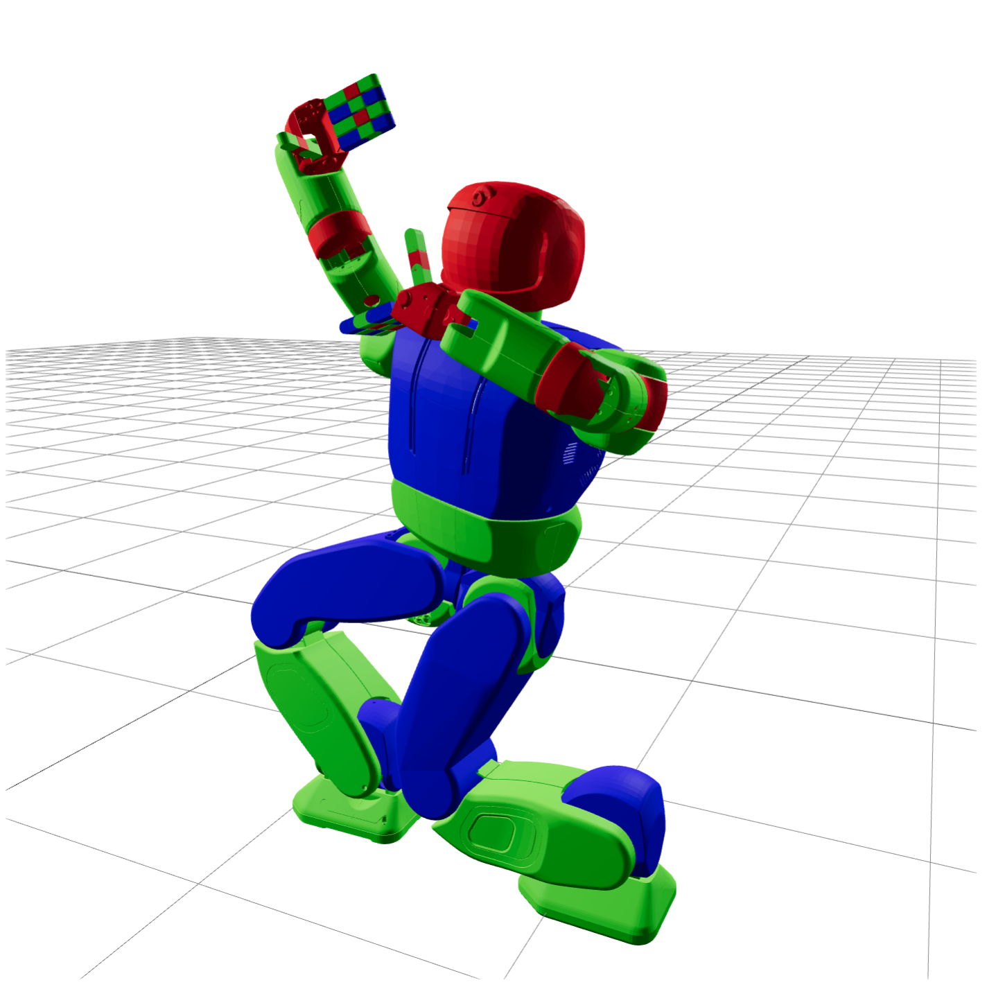
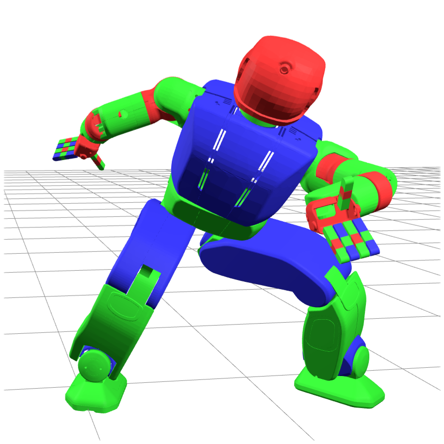
Hubo must reach a right-hand target with feet flat, center of mass above their support hull, joint limits and collision avoidance. Use 100 targets and a nominal stable start, not arbitrary random starts. The simulated arm geometry is modified to match the analytic model; this is not a hardware validation of the original Hubo.
IPOPT inequality-stability success is 97% new versus 70% old, with mean time 1.26 versus 3.45 seconds. With equality stability both achieve 96% and similar times (1.61/1.65 s). SNOPT fails; NLopt is slower and less reliable. The old formulation needs 10⁻⁴ feasibility tolerance. NLopt uses clipping with ε=10⁻⁶; the same clipping harms IPOPT.
The paper counts 34 total and 22 residual degrees of freedom in prose but 31/19 in Table I, a three-DOF difference matching the neck mentioned in the text. It does not explicitly reconcile these counts, so both source statements are retained.
V-F Scaling with the Number of Redundant Degrees of Freedom
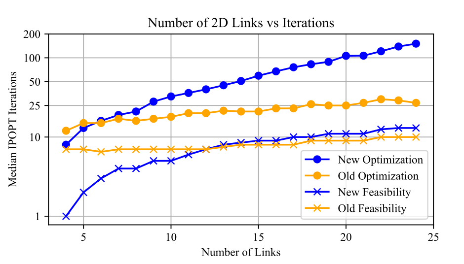
Synthetic planar and spatial chains hold overall scale approximately fixed while adding joints. These tests omit collision avoidance and separate pure feasibility from joint-centering optimization.
V-F 1 2D Setup
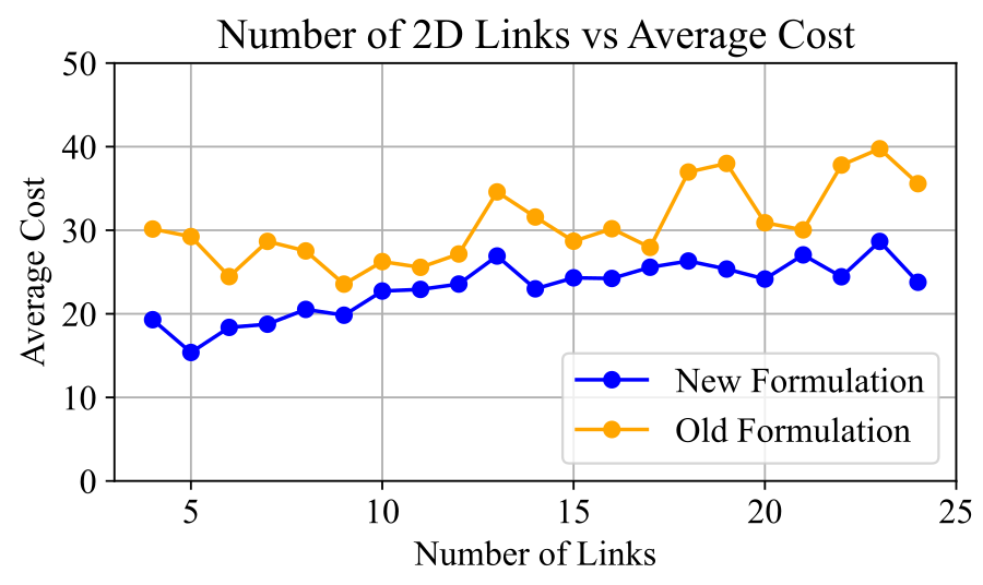
Planar chains have equal-length links and a three-joint analytic tail; earlier joints become redundancy coordinates. Use 300 targets per chain length. The new formulation finds lower costs but its optimization iterations grow faster; the old formulation becomes more iteration-efficient at high redundancy. Both exceed 95% success after broadening angle bounds to ±2π.
V-F 2 3D Setup
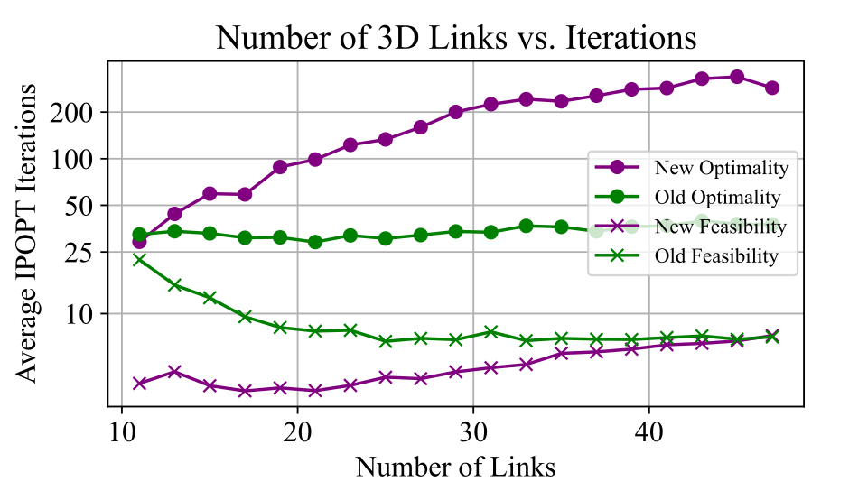
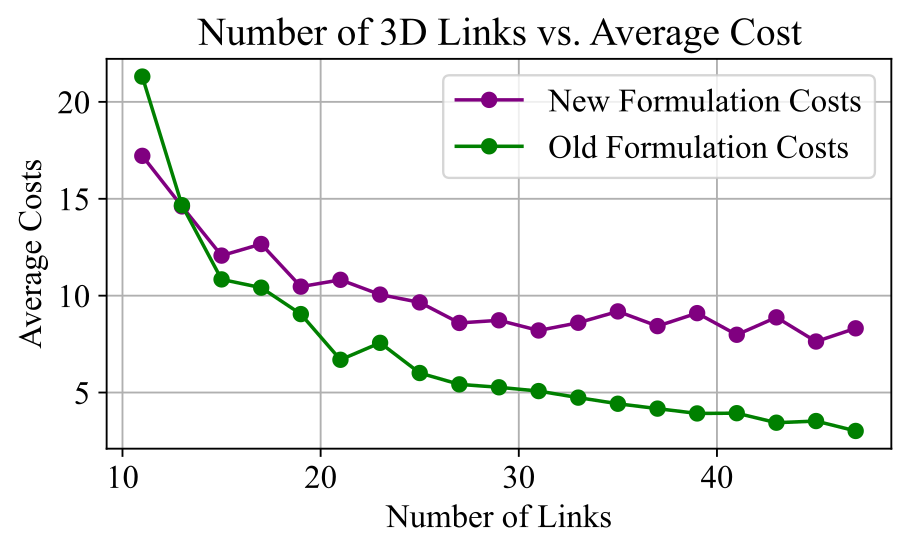
Spatial chains end in an iiwa-like seven-joint tail, with 200 targets per length. Both formulations reach 100% success at fifteen or more joints; below that, the new remains at 100% while the old drops to roughly 90% for eleven joints.
The new cost landscape becomes much harder with added joints, yielding worse costs and many more optimization iterations. Pure feasibility stays inexpensive, and the old catches up beyond about forty joints. Plots exclude failed solves; a 30-second timeout retains the best feasible incumbent, and the reported optimality tolerance is 10⁰. These conditions limit near-optimality claims.
VI Discussion
The framework is useful when a differentiable analytic IK map exists and feasibility dominates. It does not uniformly improve runtime or cost, and fixed branches, singularities and domain management remain consequential. Reported near-10⁻¹⁷ tolerances concern the analytically enforced kinematic equality, not a universal accuracy guarantee for every collision/stability constraint.
Automatically generated IK code needs differentiation and intermediate-domain probes before use here. Replacing analytic IK with numerical, algebraic or learned differentiable maps is proposed future work, not demonstrated.
VII Acknowledgements
The authors acknowledge Hongkai Dai and Seiji Shaw, and support from Amazon, the NSF, an NSF graduate fellowship and the Robotics and AI Foundation.
Appendix A Implementation of the Analytic IK Mappings
Hand-written Python mappings support Drake automatic differentiation and expose intermediate values before domain clipping. The iiwa mapping from Faria et al. mainly needs arccos clipping and unclipped probes; generated IK packages were not directly compatible with both requirements.
A.1 PR2 Analytic IK
The PR2 mapping revises Ramezani and Williams, using the first joint as redundancy. Solving sine and cosine jointly removes extraneous candidates and yields eight branches indexed by three signs. Equations 6–16 retain the full derivation, including the spherical-wrist branch transform.
Equations 6–16
| (6) |
| (7) | |||
| (8) | |||
| (9) | |||
| (10) |
| (11) |
| (12) | |||
| (13) |

Original selectable MathML (source has misplaced frame superscripts)
| (14) |

Original selectable MathML (source has misplaced frame superscripts)
| (15) |
| (16) |
A.2 Hubo Analytic IK
Published Hubo IK assumes an idealized intersecting-axis arm; the real elbow offset can cause centimeter-scale errors. The simulation URDF is changed to that idealized geometry. The implementation also removes conditional angle wrapping through a two-argument arctangent, with zero scale remaining singular.
The displayed definitions x=a sinθ, y=a cosθ and the prose arctan2(ay,ax) require care about argument convention; under the usual arctan2(y,x) convention, this is not the direct inversion of those definitions. The source is preserved rather than silently correcting its formula.
Equations 17–18
| (17) | |||
| (18) |
Appendix B Implementation of the Global MICP IK Baseline
Global-IK relaxes rotation bilinearities with mixed-integer convex constraints. Collision avoidance requires robot spheres to fit inside a union of convex free-space polytopes. Clique-cover region generation automates that decomposition using a dummy point robot in task space.
More sampled scene coverage creates many additional binary variables and does not translate directly into full robot coverage: narrow polytopes may not contain collision spheres. Fast/precise settings request 70%/85% scene coverage and different rotation-relaxation resolutions. The main text reports about 1 cm average precise pose error, while this appendix describes millimeter-scale accuracy; the edition keeps those distinct descriptions.
Table V compares four convex posture/link proxies over 100 targets. Squared link deviation reduces true joint-centering cost to 5.53 but takes 289 seconds versus 123 for posture cost. This is an approximation under relaxed kinematics, not exact equivalence to optimizing the original joint-space objective.
Equations 19) (20–20

Original selectable MathML (source has misplaced frame superscripts)
| (19) | |||
| (20) |
| Iris | Coverage | Polytopes | Total Planes | C-space Covered |
|---|---|---|---|---|
| IrisNP | 0.70 | 16.3 | 208 | 0.755 |
| 0.85 | 27.9 | 356 | 0.827 | |
| 0.95 | 47.9 | 615 | 0.881 | |
| IrisNP2 | 0.70 | 18.2 | 239 | 0.713 |
| 0.85 | 33.5 | 443 | 0.810 | |
| 0.95 | 54.7 | 771 | 0.884 | |
| IrisZO | 0.70 | 19.1 | 364 | 0.831 |
| 0.85 | 32.2 | 853 | 0.880 | |
| 0.95 | 73.1 | 1935 | 0.942 |
| Cost | Runtime (sec) | True Cost | Success Rate |
|---|---|---|---|
| e Posture Cost | 123 | 8.61 | 0.84 |
| Link Cost () | 131 | 6.06 | 0.88 |
| Link Cost () | 227 | 6.12 | |
| Link Cost () | 289 | 5.53 |
Appendix C Further Details on Setup of Experiments
The appendix specifies objectives, target/start distributions and sampling baselines. These protocol choices are essential to interpreting the headline rates.
C.1 Common Costs and Constraints
Quadratic joint costs penalize bounded joints or deviation from a nominal configuration. Drake’s minimum-distance constraint uses pairwise convex-geometry distances through FCL/libccd, with gradients. Both formulations use Euler-angle end-effector orientation constraints to reduce representation confounding.
C.2 Arm on a Table
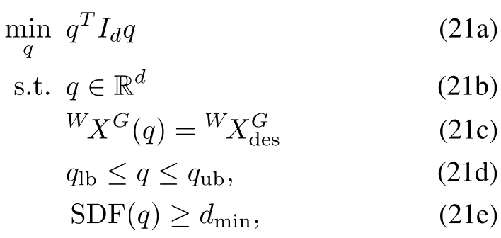
Use a 1 mm collision clearance. Target poses come from collision-free, joint-limit-respecting configurations, guaranteeing task feasibility. Initial guesses may collide or exceed limits, but correspond to the same physical configuration in both formulations. The 100×100 design reuses targets; it is not 10,000 independent target scenes. Sampling uses 500 redundancy/branch candidates with eight iiwa branches.
Equations 21a) (21b) (21c) (21d) (21e–21e
Original selectable MathML (source has misplaced frame superscripts)
| (21a) | ||||
| (21b) | ||||
| (21c) | ||||
| (21d) | ||||
| (21e) | ||||
C.3 Grasp Selection
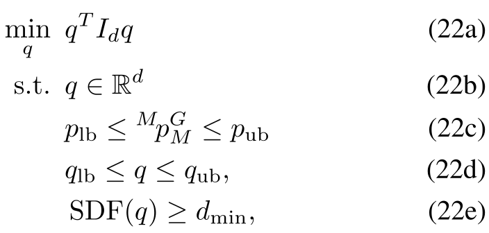
Allow the gripper center to move ±0.035 m along the mug axis while its transverse coordinates are fixed. Mug targets are generated from valid robot configurations. Starts obey joint limits but may collide. Sampling grids orientation, axial displacement, redundancy and branch index; it is not uniform sampling of joint-space volume.
Equations 22a) (22b) (22c) (22d) (22e–22e
Original selectable MathML (source has misplaced frame superscripts)
| (22a) | ||||
| (22b) | ||||
| (22c) | ||||
| (22d) | ||||
| (22e) | ||||
C.4 A Basic Mobile Manipulator
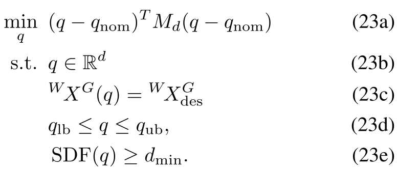
Only arm joints are penalized, relative to a nominal configuration that avoids straight-arm singularity; base variables carry zero cost. Both targets and starts are collision-free, with targets near the table. Base x/y/yaw plus one arm parameter define the four-dimensional sampling space.
Equations 23a) (23b) (23c) (23d) (23e–23e
Original selectable MathML (source has misplaced frame superscripts)
| (23a) | ||||
| (23b) | ||||
| (23c) | ||||
| (23d) | ||||
| (23e) | ||||
C.5 A Bimanual Mobile Manipulator
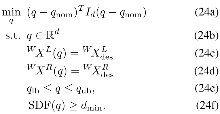
PR2 arm limits occupy less than 2% of each seven-angle torus, versus roughly 25% for iiwa; together they leave under 0.05% before collision checks. The first-joint redundancy coordinate is itself tightly bounded. Sampling restricts base x/y to ±0.5 m around the hand-target midpoint and samples lift and both shoulder parameters.
Equation 24 prints an identity-matrix cost, while its explanatory text specifies a matrix with zero weights outside arm joints. That notation inconsistency is retained; the prose describes the intended arm-only weighting.
Equations 24a) (24b) (24c) (24d) (24e) (24f–24f
Original selectable MathML (source has misplaced frame superscripts)
| (24a) | ||||
| (24b) | ||||
| (24c) | ||||
| (24d) | ||||
| (24e) | ||||
| (24f) | ||||
C.6 Humanoid Stability
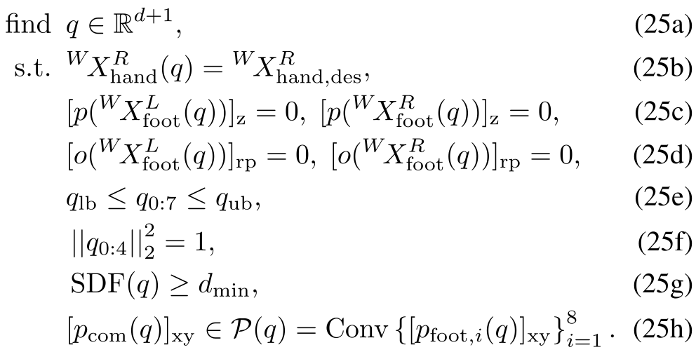
Static stability requires the horizontal center of mass inside the convex hull of eight foot corners. Convex weights give one linear and one nonlinear equality. An alternative checks all 56 three-corner triangles, both windings, and takes a maximum of edge-slack minima; Equations 26–29 preserve the exact inequality construction. This addresses static support on flat ground, not dynamic balance.
The old torso orientation uses a unit quaternion; the new uses Euler angles. Feasible-domain initialization and −μ log barrier terms protect reachability and avoid recurring singular arm configurations. Targets vary torso position/yaw and arm joints before collision rejection. Domain protection is necessary in this experiment and cannot be replaced indiscriminately by clipping.
Equations 25a) (25b) (25c) (25d) (25e) (25f) (25g) (25h–29
Original selectable MathML (source has misplaced frame superscripts)
| (25a) | ||||
| (25b) | ||||
| (25c) | ||||
| (25d) | ||||
| (25e) | ||||
| (25f) | ||||
| (25g) | ||||
| (25h) | ||||
| (26a) | ||||
| (26b) | ||||
| (27) |
| (28) |
| (29) |
C.7 2D Scaling
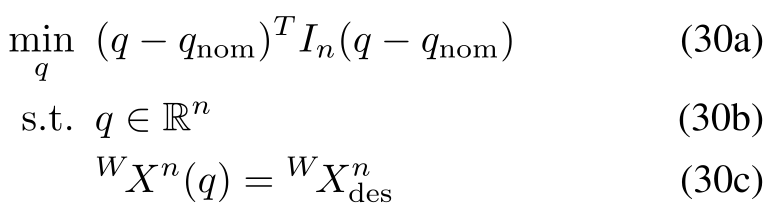
The last three planar joints are solved analytically from the target; Equation 32 expresses tail reachability. Targets lie within radius 1−2/n, with independent random starts and nominal configurations. Bounds of ±π created boundary traps, so both methods use ±2π. These artificial bounds and the collision-free model delimit the scaling result.
Equations 30a) (30b) (30c–32
Original selectable MathML (source has misplaced frame superscripts)
| (30a) | ||||
| (30b) | ||||
| (30c) | ||||

Original selectable MathML (source has misplaced frame superscripts)
| (31) |

Original selectable MathML (source has misplaced frame superscripts)
| (32) |
C.8 3D Scaling
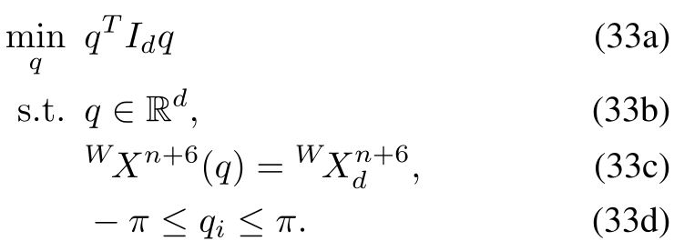
Table VI preserves the spatial chain’s DH parameters and constant total-length construction. The last seven joints are replaced by iiwa analytic IK with a randomly fixed branch. Two hundred feasible targets per length use positions in [−0.3,0.3]³ and random orientations, with independently sampled joint starts.
| link | |||
| 0 | 0 | ||
| 1 | 0 | 0 | |
| 2 | 0 | ||
| 3 | 0 | 0 | |
| 4 | 0 | ||
| 5 | 0 | 0 | |
| . . . | |||
| 0 | |||
| 0 | 0 | ||
| 0 | |||
| 0 | 0 | ||
| 0 | |||
| 0 | 0 | ||
| 0 | |||
Equations 33a) (33b) (33c) (33d–33d
Original selectable MathML (source has misplaced frame superscripts)
| (33a) | ||||
| (33b) | ||||
| (33c) | ||||
| (33d) | ||||