Overview
This edition covers all 14 pages of arXiv v4, dated 28 May 2026, including the appendix. Xunlan Zhou and Hongrui Zhao contributed equally. The RSS 2026 proceedings verify the title and authors; the author project page links code and demonstrations.
At a glance
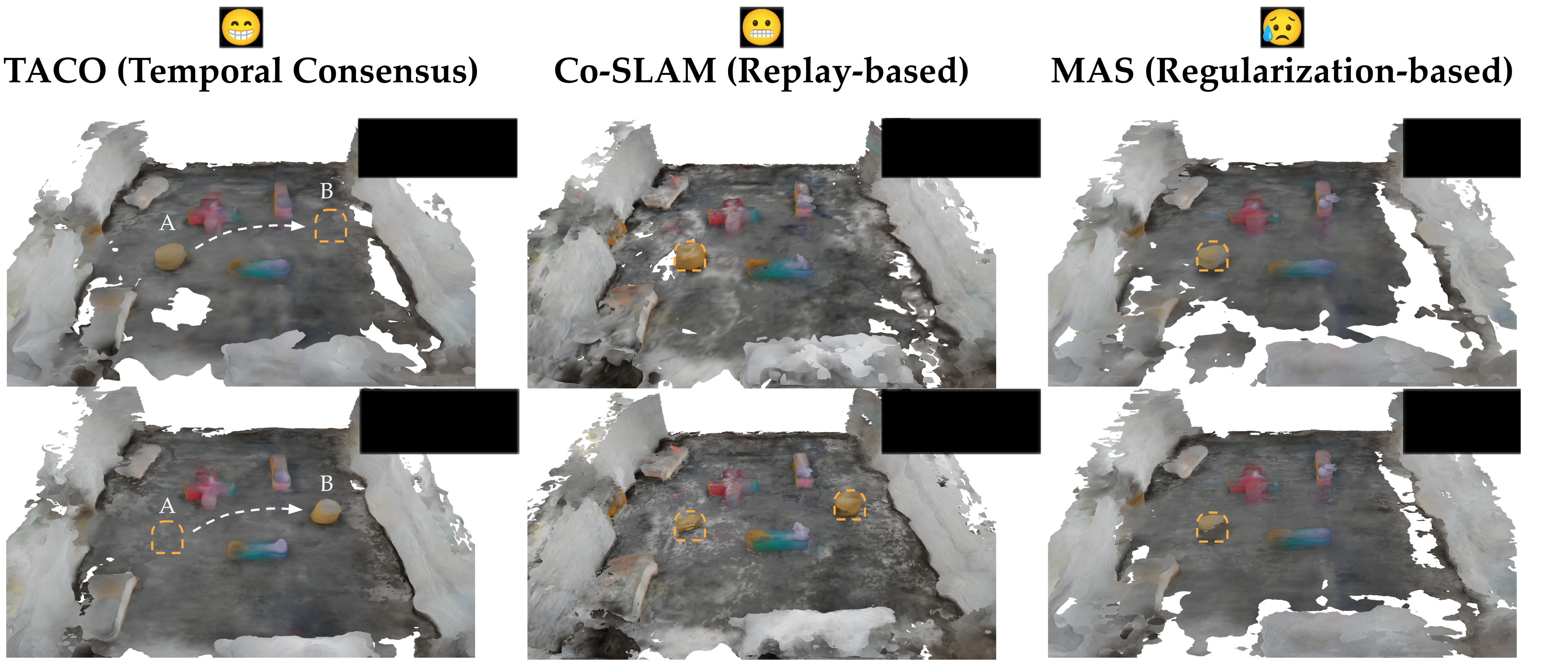
TACO updates a neural scene map from current RGB-D observations while retaining a frozen past model rather than replaying old frames. An importance-weighted consensus target protects influential historical parameters, while weakly supported ones can change. This addresses both forgetting of unchanged geometry and stale geometry after objects move.
The method matches strong static-scene baselines and improves a staged dynamic simulation over MAS: F1 at 5 cm rises from 73.43% to 78.05%. Hardware results are qualitative. CPU resident memory is 1,864.5 MB versus 4,165.1 MB for full-replay Co-SLAM; runtime and GPU memory are not reported.
I Introduction
Neural implicit maps encode color and geometry compactly, but online training often needs stored keyframes to avoid forgetting. In changing rooms, replay also forces the map to explain obsolete observations, creating duplicate objects or “ghosts.” Strong regularization can prevent those outdated surfaces from being revised.
TACO treats a previous map snapshot as a temporal neighbor. Current and historical parameter importance determine their agreement target, with a threshold removing weak historical constraints. The goal is selective retention, not exact preservation of every old reconstruction.
II Related Works
Replay, parameter regularization, isolation and distillation address different forms of forgetting. Continual Neural Mapping and UNIKD bring these ideas to implicit scenes, but preserving earlier reconstructions can conflict with genuine object motion.
Distributed neural mapping already uses consensus to reconcile separate robots. TACO transfers that idea to successive states of one model. Unlike frequency-based importance in RAMEN, it adopts Memory Aware Synapses-style output sensitivity. This is a parameter-importance proxy, not a calibrated estimate that a particular surface is unchanged.
III Preliminaries
The implementation builds on Co-SLAM and an approximate method-of-multipliers optimizer. The following equations retain the source’s full mapping and optimization definitions.
III-A Neural Implicit Mapping with Co-SLAM
Co-SLAM combines a multiresolution hash grid with geometry and color decoders. The geometry network takes interpolated features and one-blob coordinate encoding, predicting a signed distance and a latent feature; the color network uses that feature and the coordinate encoding to predict RGB.
Camera rays are sampled in 3D. Color and depth are weighted averages of predictions, with sigmoid weights concentrated near the zero level of the signed-distance field. Training combines photometric, depth, SDF, free-space and smoothness losses. Detailed loss definitions and weighting are inherited from Co-SLAM rather than restated here.
Equations 1–5
| (1) |
| (2) |
| (3a) | ||||
| (3b) | ||||
| (4) |
| (5) |
III-B Constrained Optimization with the Method of Multipliers
For a linear equality constraint, the augmented Lagrangian adds a dual disagreement term and a quadratic penalty to the reconstruction loss. Each iteration approximately minimizes this objective in the map parameters, then accumulates the remaining constraint error in the dual variable.
The primal step uses a few stochastic-gradient steps rather than an exact minimizer. The method-of-multipliers reference motivates the procedure; the paper supplies no convergence theorem for the later nonconvex, changing-target neural-map problem.
Equations 6–8b
| (6) |
| (7) |
| (8a) | ||||
| (8b) | ||||
IV Temporal Consensus Optimization for Continual Neural Mapping
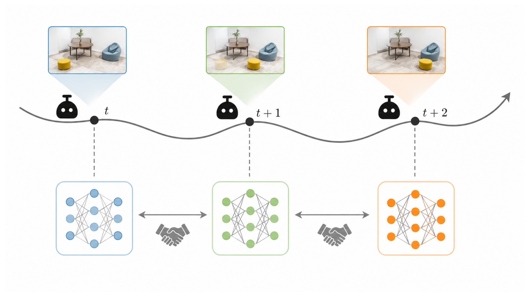
Temporal consensus replaces coordination among several robots with agreement between the current neural map and frozen earlier maps. Historical model parameters and their importance values are retained; old RGB-D frames are not.
IV-A Problem Formulation
Only the current observation stream trains the map. Two goals compete: revise geometry contradicted by new evidence, and preserve useful reconstruction outside the current view. Uniform agreement with an old model can obstruct the first; unconstrained streaming updates can destroy the second.
IV-B Importance-Weighted Temporal Consensus
The principal formulation uses one predecessor. Its consensus target is a coordinate-wise weighted mean of current and historical parameters. Before each primal update, weights and the target are recomputed from the previous iterate; the target is held fixed during that update, followed by dual ascent. After a finite number of iterations, the result becomes the new map.
The penalty ρ controls consensus strength. Adaptation relies on the weighting, mask and finite approximate updates: exact equality with the self-dependent target would force a parameter back to its old value wherever historical weight remains positive. The paper does not establish convergence or a guarantee against forgetting.
Equations 9–14
| (9) |
| (10) |
| (11) |
| (12) |
| (13) |
| (14) |
IV-C Importance Estimation for Temporal Consensus
Importance accumulates absolute gradients of a proxy equal to the mean squared magnitude of rendered color and depth. It needs no ground-truth labels, but it measures sensitivity of those outputs, not their correctness. Shared network parameters can affect multiple regions, so parameter masking is not explicit object-level change detection.
The current and saved importance vectors are jointly scaled so their average sum matches ρ, then used as diagonal weights. A threshold β zeros small historical weights. The common scaling cancels from the unmasked weighted-average target, but affects which weights survive the threshold; ρ also enters the augmented penalty.
The formulas leave the all-zero importance denominator and zero-weight inverse unspecified. Initialization, snapshot cadence, optimizer budgets and numerical safeguards are not fully documented in the paper. The appendix calls the masking threshold τ, while the main derivation uses β.
Equations 15–18
| (15) |
| (16) |
| (17) |
| (18) |
Equations 19
| (19) |
V Experiments and Results
All comparisons are implemented within Co-SLAM. Static tests use eight Replica scenes, two ScanNet scenes and a larger Gibson example. Dynamic tests stage object relocations in Habitat synthetic scenes and in a TurtleBot room.
Baselines include EWC/MAS regularization, CNM replay, a ten-keyframe replay buffer (KR), and UNIKD distillation, plus Co-SLAM with and without replay. These last two are useful reference conditions rather than mathematical performance bounds; replay can fail when past observations become stale. Dynamic evaluation narrows the comparison to MAS and replay Co-SLAM.
V-A Results on Static Simulated Scenes
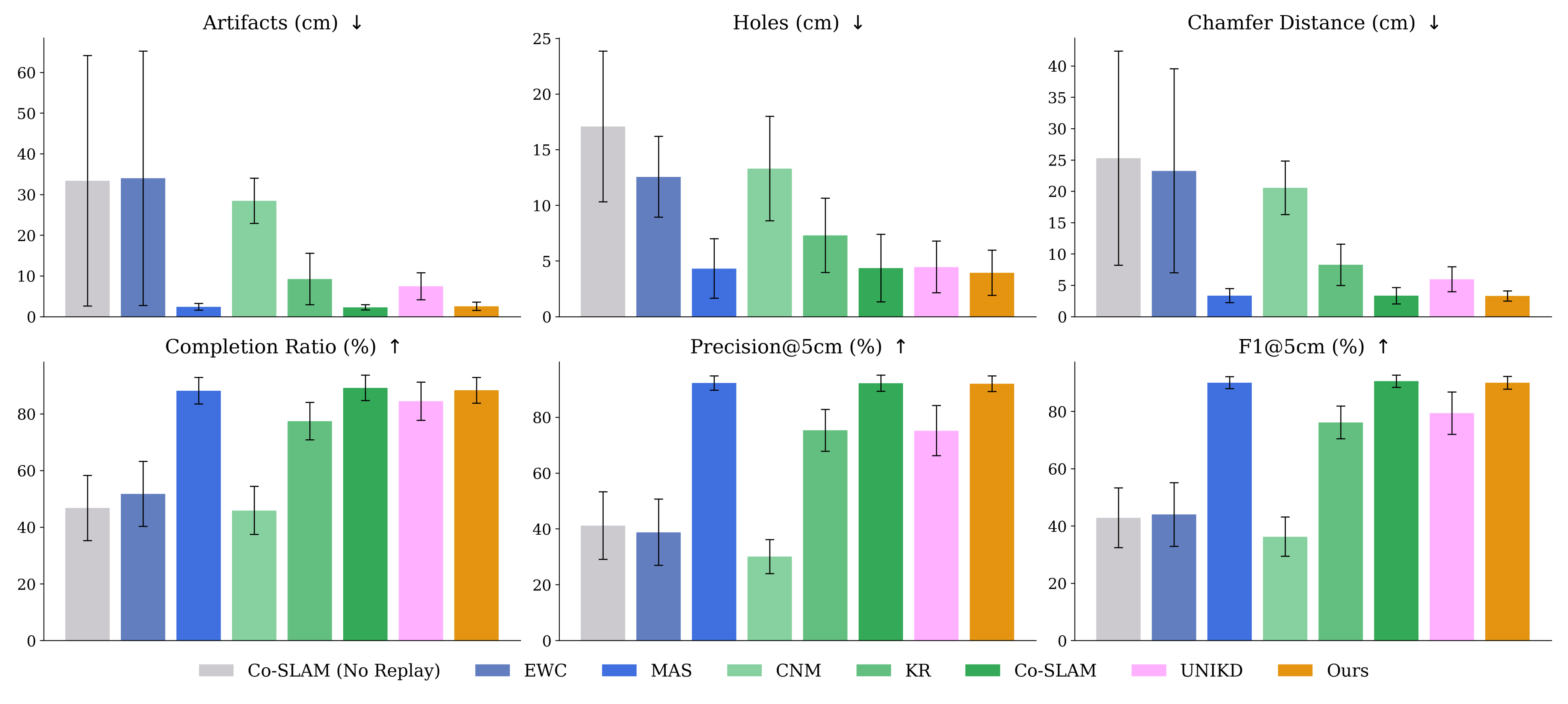
Across six aggregate Replica metrics, TACO lies near replay Co-SLAM and MAS, while EWC and no-replay Co-SLAM suffer substantial reconstruction errors. Figure 3 shows aggregate bars and error bars; scene-level values and the error-bar definition are not tabulated.
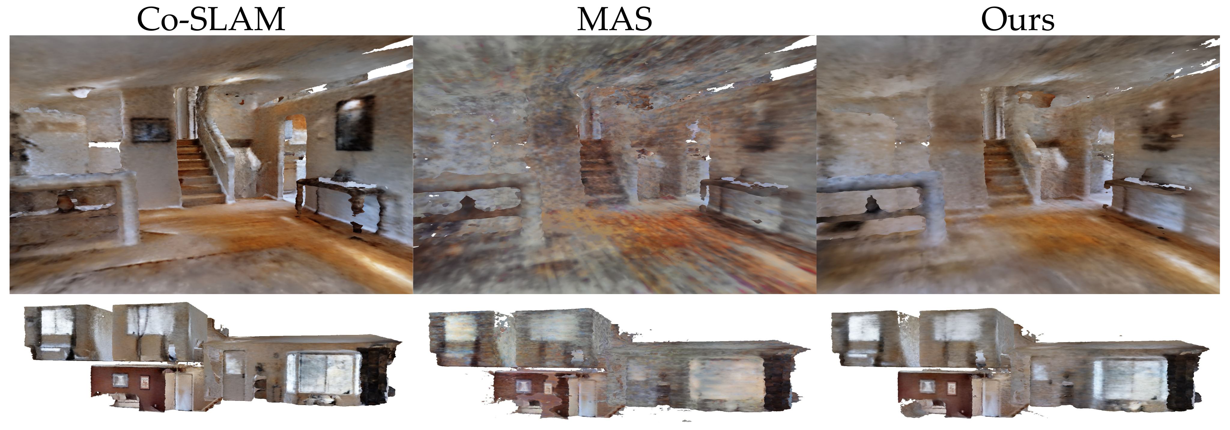
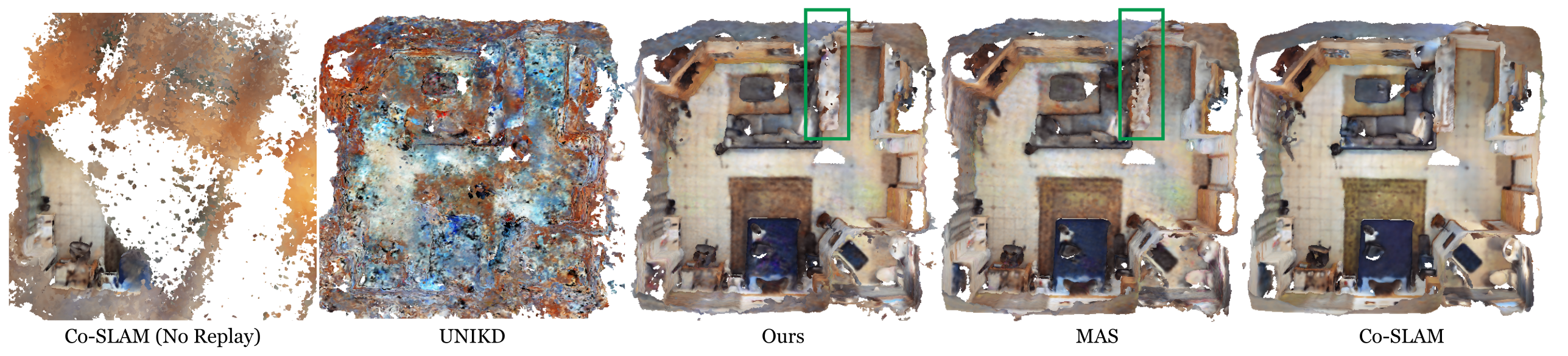
In the larger Gibson scene, TACO has more coherent geometry than MAS, but both show appearance inconsistency relative to replay Co-SLAM. This is a qualitative scalability example; no scene-size, speed or scaling curve is supplied.
V-B Results on Dynamic Simulated Scenes
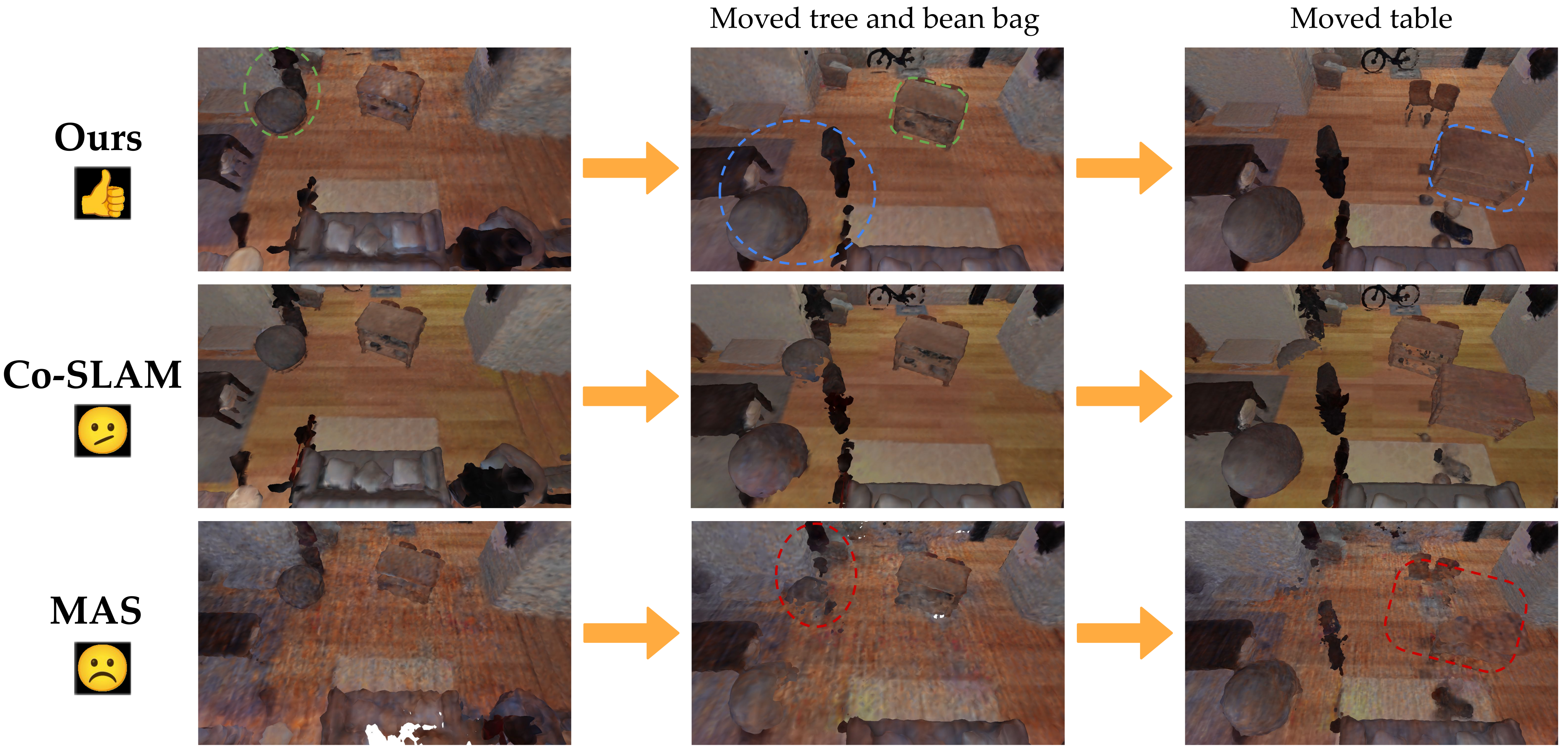
The simulated sequence first moves a beanbag and potted tree, then moves a table and scatters tableware. Most of the room stays fixed. TACO revises the moved objects while preserving the surrounding mesh; replay Co-SLAM produces old/new copies, and MAS shows tearing and fragmentation.
Against MAS, artifacts fall from 8.53 to 6.38 cm, completion rises from 71.41% to 74.37%, and F1 at 5 cm rises from 73.43% to 78.05%. Co-SLAM is shown visually but has no row in Table I. Dataset size, repeated-run uncertainty and stage-wise numerical scores are not reported.
V-C Continual Mapping in Dynamic Real-World Environments
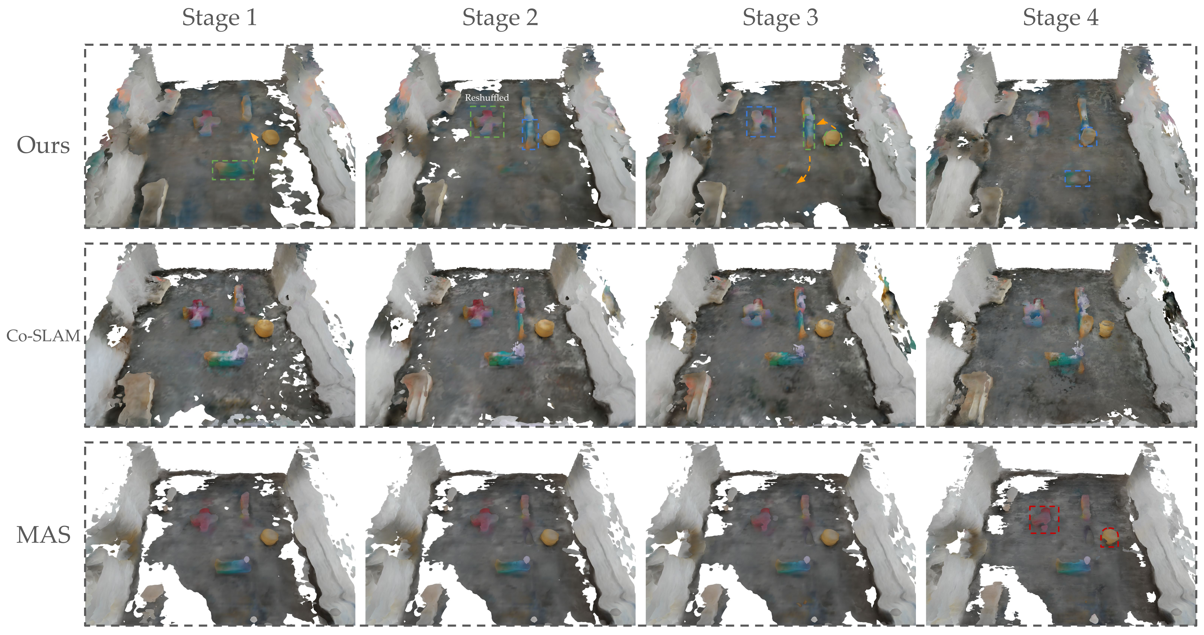
The opening experiment moves a yellow stool between two locations. A second experiment shows four scene configurations: cubes are moved, reshuffled, and partly returned while the stool occupies their former position. TACO’s meshes track these changes more cleanly than the two selected baselines.
These are controlled relocations followed by reconstruction, rather than a benchmark of continuously moving people or objects. The hardware evidence is visual: no geometric ground-truth scores, localization-error evaluation, update latency or repeated-trial statistics are supplied.
V-D Analysis of Memory Usage
Measured CPU resident set size is 1,864.5 MB for TACO, 4,165.1 MB for full replay, 1,912.4 MB for KR, 1,945.1 MB for UNIKD and 1,800.6 MB for online MAS. TACO uses about 55.2% less than full replay, but slightly more than MAS.
Replay-free does not mean state-free: a map snapshot, importance vectors and dual state remain. The table gives process-level CPU memory, without a component breakdown, GPU-memory measurement, latency benchmark or long-horizon growth curve.
VI Conclusion
The contribution is a practical temporal-consensus alternative to frame replay, with encouraging preservation of static geometry and adaptation after staged scene changes. The strongest numerical dynamic result is the comparison with MAS; hardware behavior and larger-scene scaling are demonstrated qualitatively.
Important limits are incomplete optimizer/runtime details, sensitivity rather than calibrated reliability, limited dynamic baselines, and no formal stability or convergence guarantee. The appendix also contains inconsistent ablation claims and one unmatched default Chamfer value, explained below with the original values retained.
Acknowledgments
Support: NSF ECCS-2438314 (CAREER) and CNS-2529645, the UC Berkeley Center for Digital Assets, and GPU resources from the NVIDIA Academic Grant.
Appendix A. Quantitative Metrics for Geometry Evaluation
Artifacts measure mean reconstructed-to-ground-truth surface distance; holes reverse that direction. Both are reported in centimeters, and their symmetric average is Chamfer distance. Lower is better.
Completion is the percentage of ground-truth points with reconstructed neighbors within 5 cm; precision reverses the sets. F1 is the harmonic mean of these 5 cm recall/precision values. These metrics complement one another: reducing spurious geometry alone can leave missing surfaces. Point sampling, alignment and aggregation details are not fully specified.
Appendix B. Results on Static Simulated Scenes
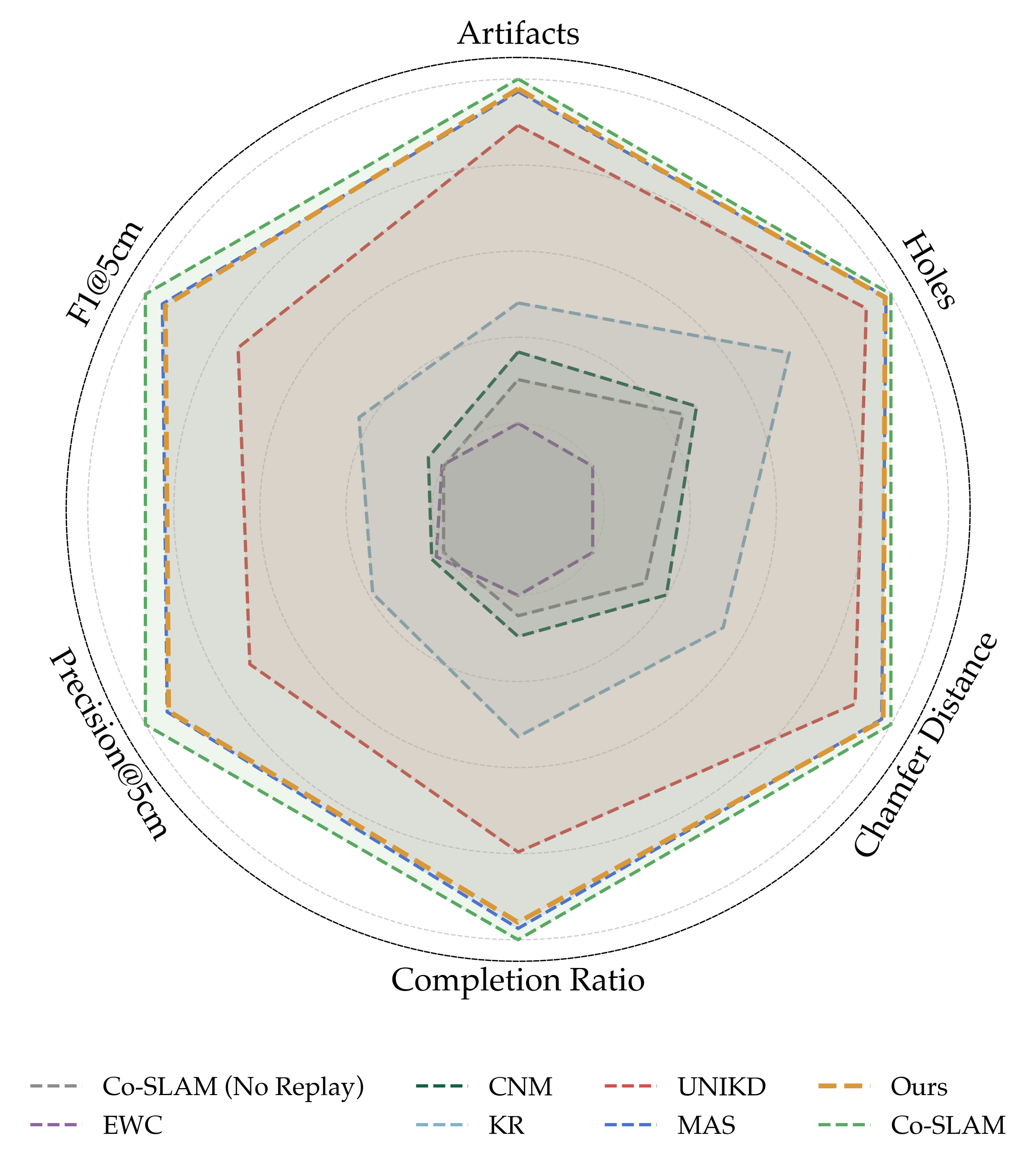
Replica results place replay Co-SLAM, MAS and TACO near the top, with KR ahead of CNM and UNIKD between weaker baselines and the leaders. These aggregate plots support competitive accuracy and coverage rather than a statistically established win on every individual scene.
The ScanNet radar plot summarizes scene0000_00 and scene0673_05 without numerical radial ticks or a stated normalization. Figure 8 shows coherent geometry and a more complete table for TACO, strong color inconsistency for UNIKD, and fragmentation without replay. The text’s broad claim that parameter regularizers all degrade should be read alongside MAS’s near-leading radar trace.
Appendix C. Ablation on Mask Mechanism
On Replica room1, threshold 10⁻⁴ gives the best listed Chamfer/F1 pair, 2.05 cm/93.65%, compared with 2.17/93.06 for threshold zero. The larger thresholds 10⁻² and 10⁻³ perform worse than no masking, contrary to the prose’s claim that adding the mask consistently improves performance.
The threshold and consensus penalty are coupled through weight scaling, but their joint sweep is not reported. Setting the threshold to zero disables threshold-based suppression; setting historical weights themselves to zero would instead remove historical influence. The source’s wording conflates these cases.
Appendix D. Ablation on the Number of Temporal Snapshots
With one to four snapshots on static Replica room1, Chamfer rises 2.50→3.51 cm and F1 falls 93.65→87.60%. One predecessor is best in this ablation. The explanation invoking obsolete dynamic geometry is plausible for changing scenes, but this table itself uses a static benchmark.
The one-snapshot row reports Chamfer 2.50, while the best threshold row in Table III reports 2.05 with the same F1 of 93.65. The paper does not reconcile their settings or values; both tables are preserved. Here K counts snapshots, whereas K in the main optimization section counts iterations.