Overview
At a glance
Intuition. Encode an image, predict how its representation changes, then try candidate actions inside that learned model. EB-JEPA packages these steps into small examples that can be trained on one accelerator, so individual design choices are easier to inspect than in a billion-parameter training system.
The library progresses from image views to video dynamics and goal-conditioned navigation. Its headline results are approximately 90–91% linear-probe accuracy on CIFAR-10 and 97% planning success in a particular Two Rooms setup. These demonstrate the included examples, not a general-purpose robot world model.
1 Introduction
The contribution is an accessible implementation and controlled experiments. Image, video and action-conditioned variants share modular encoders, predictors, regularizers and planners. Small examples make it possible to change one component and inspect the result before attempting a larger system. The paper’s representation-learning motivation does not make pixel reconstruction categorically useless; the experiments test particular objectives and tasks.
2 Related Work
Joint-Embedding methods.
The library focuses on JEPAs that prevent collapse through explicit regularization, rather than representing every JEPA design. VICReg and SIGReg are implemented examples. Teacher/stop-gradient approaches and pixel-prediction methods form related alternatives, not interchangeable implementations of the same loss.
World models for planning.
Related latent world models learn dynamics for planning or reinforcement learning. EB-JEPA aims at readable, self-contained experiments rather than state-of-the-art results on complicated benchmarks.
3 Preliminaries: A Unified JEPA Framework
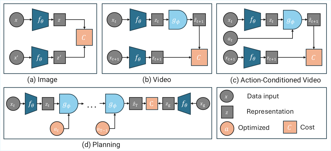
An energy is a compatibility score: an observed context and a plausible target should receive a low value. Here it is computed from error between a predicted embedding and an encoded target. A regularizer stops the encoder from making every target the same easy-to-predict vector. For image views, the predictor can be identity. Video introduces temporal prediction. Action-conditioned video additionally encodes the control input, allowing different actions from the same state to lead to different predicted states.
Equations 1–4
| (1) |
| (2) |
| (3) |
| (4) |
A unified energy formulation.
A common expression combines an encoder, a predictor and an optional conditioning encoder. Removing action conditioning gives a video predictor; removing temporal prediction gives an image-view example. The shared equation is a software and conceptual interface, while the data and regularization needs differ.
Equation 5
| (5) |
Regularization: Preventing Collapse.
VICReg encourages variation across examples and reduces covariance between coordinates. SIGReg instead tests whether randomly projected embeddings resemble an isotropic Gaussian distribution. Image and video examples may apply these losses after a learned projection head. A spread-out embedding avoids a constant-vector shortcut, but useful dynamics can still require additional constraints; Gaussianity alone does not guarantee a suitable representation for every task.
Equations 6–8
| (6) |
| (7) |
| (8) |

4 Training and Planning with World Models
Multistep Rollout Training.
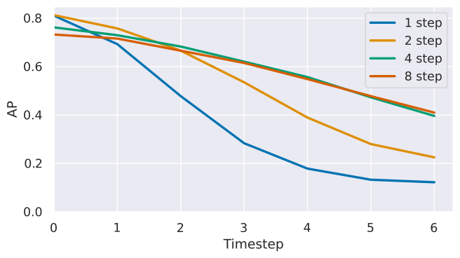
A one-step predictor trained only on freshly encoded true states can fail when repeatedly fed its own predictions. Multistep training includes recursively predicted states in the loss, bringing training closer to rollout-time use. The horizon and treatment of gradients through successive steps are important implementation choices.
Equations 9–11
| (9) |
| (10) |
| (11) |
Additional Regularizers for World Models.
The action-conditioned example adds temporal smoothness and inverse dynamics, which predicts an action from consecutive states. The latter discourages encoding only a static background that is predictable but unrelated to the controls. These constraints address a different shortcut from total representation collapse.
Equations 12–13
| (12) |
| (13) |
Goal-Conditioned Planning.
To reach a goal image, the planner samples action sequences, rolls them through the latent predictor and scores their distances from the goal representation. Model Predictive Path Integral planning refines the proposals by favoring lower-cost sequences. This implementation sums costs across the horizon rather than checking only the final predicted state, and replans as new observations arrive.
Equation 14
| (14) |
5 Experiments
Experimental Setup.
The three examples are CIFAR-10 image representation learning, MovingMNIST video prediction and Two Rooms goal-conditioned navigation. The code includes alternative encoders, predictors, regularizers and sampling-based planners. Appendix tables fix the actual training and planning settings for each comparison.
Image Representation Learning.
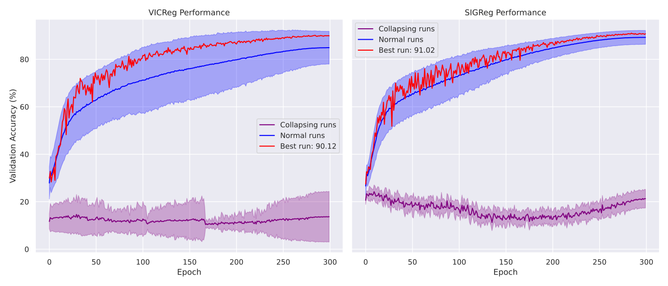
Linear probes reach roughly 90–91% on CIFAR-10. A learned projection head improves the tested regularizers by about three percentage points, and its preferred dimensions differ between VICReg and SIGReg. The comparison uses a simple hyperparameter search; it illustrates tuning behavior rather than proving one regularizer universally superior.
| Best acc. | Average acc. | w/o Projector | Hyperparams | Best projector | |
|---|---|---|---|---|---|
| SIGReg | 91.02% | 89.22% | -3.3 points | 1 | 2048128 |
| VICReg | 90.12% | 84.90% | -2.9 points | 2 | 20481024 |
| SIGReg | VICReg | |||
|---|---|---|---|---|
| Rank | Hyperparameters | Accuracy | Hyperparameters | Accuracy |
| 1 | 90.88% | std = 1, cov = 100 | 90.12% | |
| 2 | 86.94% | std = 1, cov = 10 | 89.93% | |
| 3 | 80.86% | std = 10, cov = 10 | 89.20% | |
| -1 | 27.20% | std = 100, cov = 100 | 10.00% | |
| SIGReg | VICReg | |||
|---|---|---|---|---|
| Rank | Dimensions | Accuracy | Dimensions | Accuracy |
| 1 | 2048128 | 91.02% | 20481024 | 90.12% |
| 2 | 40961024 | 91.00% | 4096512 | 90.10% |
| 3 | 204864 | 90.99% | 10241024 | 90.05% |
| 4 | 512256 | 90.99% | 2048512 | 90.03% |
| 5 | 409664 | 90.96% | 40961024 | 90.02% |
| N/A | None | 87.75% | None | 87.27% |
Video Prediction.
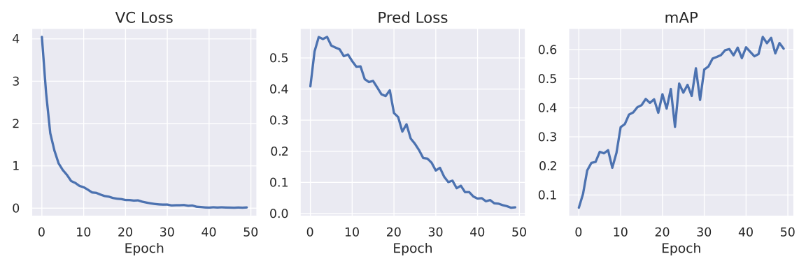
MovingMNIST results favor training on longer recursive prediction horizons over a one-step-only setup. Predicted embeddings are evaluated through a downstream detection probe, with reconstructed clips providing a visual check. The measured improvement is specific to the included dataset and setup.



Action-Conditioned Video-JEPA.
In random-wall Two Rooms navigation, the best configuration reaches 97% success. Removing inverse dynamics reduces success to 1%, consistent with the static-shortcut issue. Other regularization ablations also reduce success. Cumulative goal distance beats final-state-only distance in this setup, even though a successful path may initially need to move away from the goal to pass through a doorway.
6 Future Directions
The small-scale examples are intended as a testbed. Scaling an observed improvement to natural videos or robots requires additional evaluation; the library does not establish that transfer automatically.
Advancing Regularization Theory.
Regularization combinations remain an open research question. Controlled ablations can help determine when coordinate diversity, temporal smoothness and inverse dynamics contribute distinct information, and when their weights need retuning.
Hierarchical World Models.
Hierarchical prediction could connect short control steps to longer-term abstractions. This is a proposed future extension here, not an evaluated hierarchy already supplied by these experiments.
Learned Cost and Value Functions.
Distances between learned states may be a poor proxy for useful progress in complicated tasks. Learned costs or values are suggested extensions for directing the planner toward task-specific outcomes.
Complementary to Large-Scale Codebases.
The intended workflow is to test a mechanism in a compact example and then investigate it in infrastructure supporting larger datasets and distributed training. EB-JEPA complements those systems rather than replacing their scaling and evaluation machinery.
7 Conclusion
EB-JEPA connects explicit regularization, latent prediction and planning in one small codebase. Its ablations show why a usable world model needs more than a low prediction loss. Its strongest contribution is an inspectable experimental starting point with stated datasets and settings.
Ethics statement
Experiments use public image/video benchmarks and procedurally generated navigation scenes. The ethics statement identifies no newly collected personal data or human-subject experiments.
Reproducibility statement
Self-contained training scripts, model implementations, evaluation code and hyperparameter tables support reproducing the examples. Two Rooms generation also records seeds; these details matter when comparing the reported success rates.
Acknowledgments
The authors acknowledge discussions and conceptual contributions from Adrien Bardes and Gaoyue Zhou.
Appendix A Hyperparameters
The preserved tables state training hyperparameters, rollout horizons, sequence lengths and planning configurations. Consult these before interpreting an ablation as changing only one factor.
| Group | Hyperparameter | VICReg | ViT Image-JEPA | SIGReg |
|---|---|---|---|---|
| Optimization | Optimizer | LARS | AdamW | LARS |
| LR schedule | 10-epoch warmup (from ) + cosine to 0 | |||
| Learning rate | 0.3 | 0.001 | 0.3 | |
| Epochs | 300 | 300 | 300 | |
| Batch size | 256 | 512 | 256 | |
| Weight decay | ||||
| Data | Dataset | CIFAR-10 | CIFAR-10 | CIFAR-10 |
| Image size | ||||
| Architecture | Encoder | ResNet-18 | ViT-S | ResNet-18 |
| Predictor | Identity | Identity | Identity | |
| Encoder output dim | 512 | 384 | 512 | |
| Projector hidden dim | 2048 | 2048 | 2048 | |
| Projector output dim | 2048 | 2048 | 128 | |
| Projector layers | 3 | 3 | 3 | |
| Loss | Loss type | VICReg | VICReg | SIGReg |
| Variance coeff. | 1 | 1 | – | |
| Covariance coeff. | 80 | 80 | – | |
| SIGReg coeff. | – | – | 10 | |
| Group | Hyperparameter | Video-JEPA | AC-Video-JEPA |
| Optimization | Learning rate | 0.001 | 0.001 |
| Epochs | 50 | 12 | |
| Batch size | 64 | 384 | |
| Weight decay | – | ||
| Data | Dataset | Moving MNIST | Two Rooms |
| Trajectory length | 10 | 17 | |
| Image size | |||
| Architecture | Encoder | ResNet-5 | IMPALA |
| Predictor | ResUNet | GRU | |
| Latent dimension | 16 | 32 | |
| Hidden dimension | 32 | 32 | |
| Encoder receptive field | 1 | 1 | |
| Predictor receptive field | 2 | 1 | |
| Loss | Rollout steps | 4 | 8 |
| Variance coeff. | 10 | 16 | |
| Covariance coeff. | 100 | 8 | |
| Time similarity coeff. | – | 12 | |
| IDM coeff. | – | 1 |
| Hyperparameter | Symbol | Value |
|---|---|---|
| Planning horizon | 90 | |
| Number of parallel samples | 200 | |
| Number of iterations | 20 | |
| Number of elites | 20 | |
| Noise scale | 2 | |
| Temperature | 0.005 | |
| Actions stepped per plan | 1 | |
| Max steps per episode | 200 |
Appendix B Planning Algorithm
The planner is a practical hybrid: it first selects a subset of low-cost trajectories, then applies exponential cost weights within that subset. Temperature controls concentration. This differs from both weighting every sampled trajectory in a pure MPPI description and uniformly fitting only elites in a basic cross-entropy method. The original algorithm is retained below.
Appendix C Extended Related Work
Diffusion-Based Planning.
Diffusion-based planners learn to generate trajectories by iterative denoising; JEPA world models instead support evaluating candidate actions through latent dynamics. The methods can be combined, but their objectives and online computations differ.