Overview
FPO++ adapts flow-matching policy gradients to robot control, with independently clipped noise-sample ratios and a reward-dependent choice of trust-region objective.
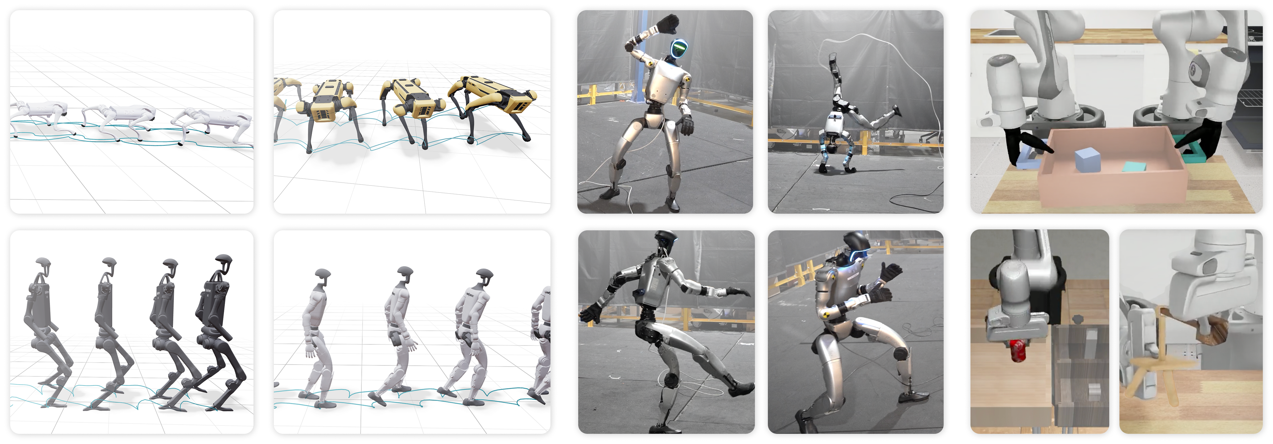
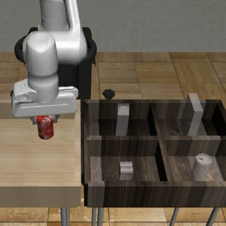
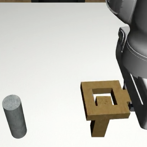
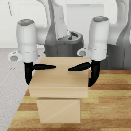
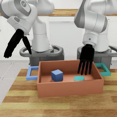
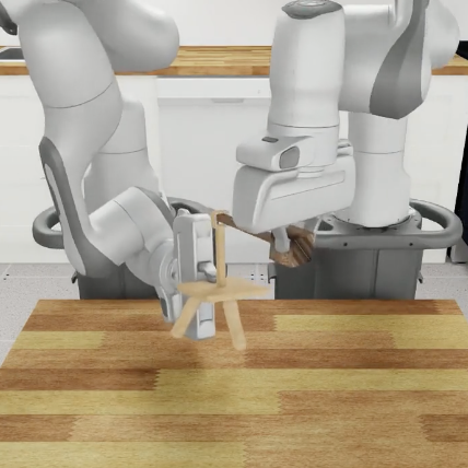
RoboMimic DexMimicGen
At a glance
FPO++ trains expressive flow policies from rewards without computing action likelihoods. Per-noise-sample ratios improve stability; an asymmetric trust region further helps dense-reward locomotion and motion tracking. Experiments include four simulated legged platforms, physical deployment on two humanoids, and simulated manipulation finetuning. The asymmetric variant is detrimental in the tested manipulation regimes, tuned Gaussian policies remain stronger on some tracking comparisons, and flow training costs more wall-clock time.
1 Introduction
Flow policies can express correlated or multimodal action distributions but make direct likelihood evaluation expensive. This work builds on flow-matching policy gradients to support locomotion, motion tracking, and reward finetuning of demonstration-trained manipulators. Its contribution is an empirically more reliable surrogate update, accompanied by physical transfer and analysis of exploration. It is not a general proof that the surrogate equals an exact action-likelihood policy gradient.
2 Background and Related Work
PPO [2] weights advantages by new/old action-likelihood ratios and clips updates. Flow and diffusion policies are useful in imitation learning but require extra work to compute such likelihoods. DPPO [7] and ReinFlow [8] instead optimize stochastic denoising-trajectory likelihoods.
Flow policy optimization uses changes in conditional flow-matching error as a surrogate ratio. It does not differentiate through environment transitions or unroll the entire sampling process during the policy update. This changes the training objective and its approximations; it does not supply an exact marginalized action density.
Equations 1–2
| (1) |
| (2) |
3 FPO++
FPO++ modifies FPO [13] in two ways: it computes and clips a separate surrogate ratio for each sampled noise/time pair, and it can penalize excessive changes on negative-advantage samples with an asymmetric objective. The latter is selected by task/reward regime.
3.1 Preliminaries
FPO estimates conditional flow-matching loss from Gaussian noise and interpolation times for each observed action. The velocity target is action minus noise along the linear interpolation. Exponentiating the old-minus-new loss approximates a likelihood ratio, and an advantage-weighted clipped objective encourages better actions. The Monte Carlo loss samples used for updates are distinct from Euler integration steps used to generate actions.
Equations 3–7
| (3) |
| (4) |
| (5) |
| (6) | ||||
| (7) |
3.2 FPO++
Original FPO exponentiates the average loss difference, creating one ratio per action and clipping all its noise/time samples together. FPO++ exponentiates each sample’s loss difference separately, sharing the action’s advantage but allowing independent clipping. At the unchanged policy, both ratios are one and their gradients agree; repeated optimization steps produce different updates.
For nonnegative advantages, ASPO uses PPO clipping. For negative advantages, it uses the quadratic penalty from Simple Policy Optimization [33], which pulls ratios back rather than merely zeroing their gradients beyond a boundary. This discourages aggressive increases in flow-matching loss. The trust-region interpretation is based on a surrogate and variational-gap argument, not a measured exact policy KL constraint.
Equations 8–10
| (8) |
| (9) |
| (10) |
3.3 FPO++ Objective
Each action receives several independently sampled noise/time pairs and a common estimated advantage. The full objective sums the per-sample ASPO contributions, then averages over on-policy observations and actions. All original formulas are retained. Manipulation experiments replace ASPO with ordinary PPO clipping while keeping the per-sample ratios, so their reported FPO++ is a task-specific configuration.
Equations 11–12
| (11) |
| (12) |
4 Experiments
The experiments cover learning from scratch, transfer of trained controllers to hardware, finetuning image-conditioned policies, and ablations against flow and Gaussian baselines. Return, task success, and wall-clock cost are separate outcomes, and the appendix documents cases where they disagree.
4.1 Locomotion Benchmarks
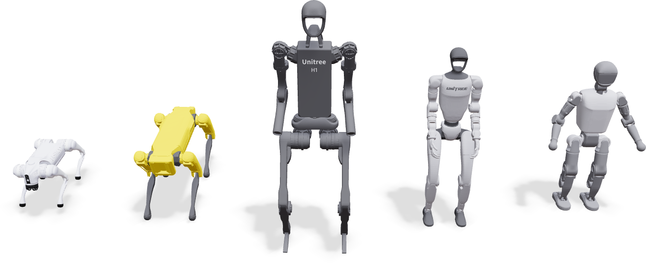
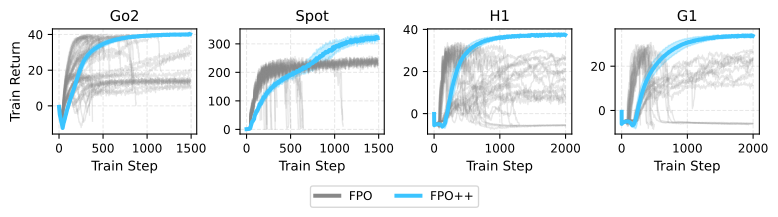
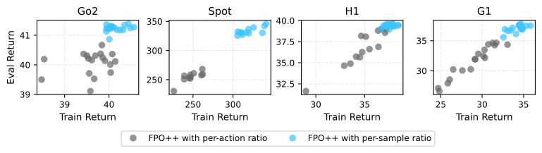
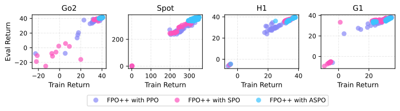
IsaacLab velocity-tracking tasks use Go2 and Spot quadrupeds plus H1 and G1 humanoids, with proprioception and commanded linear/angular velocities. Vanilla FPO often collapses or stalls despite sweeps over learning rate, clipping, and Monte Carlo count. FPO++ learns and maintains stronger returns across five seeds. This supports stability in these environments rather than a guarantee across arbitrary high-dimensional control tasks.
4.2 Humanoid Sim-to-real
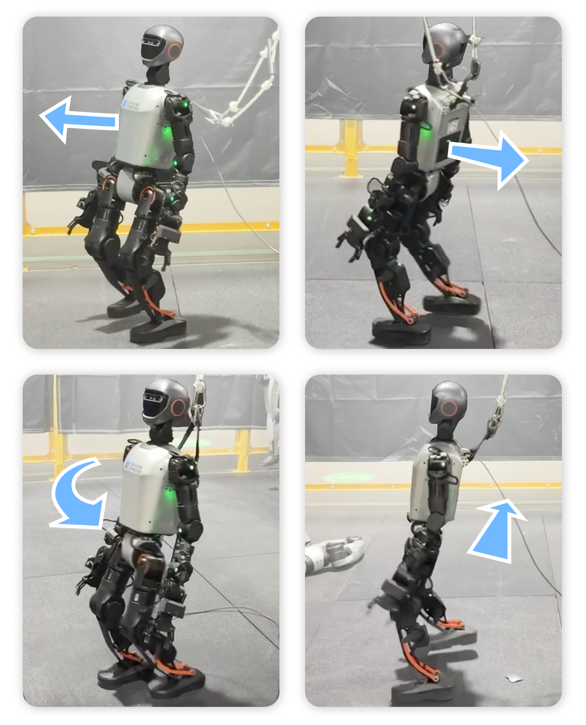
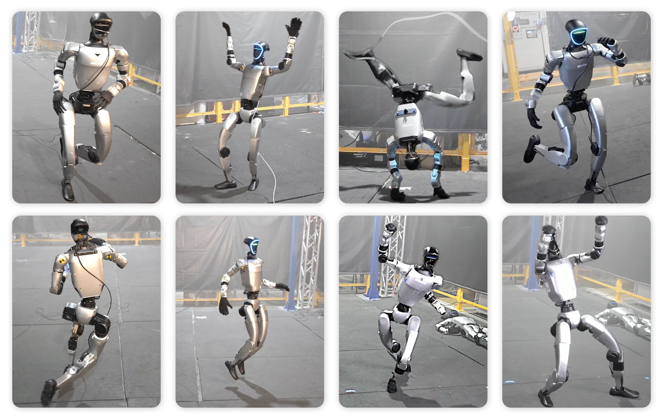
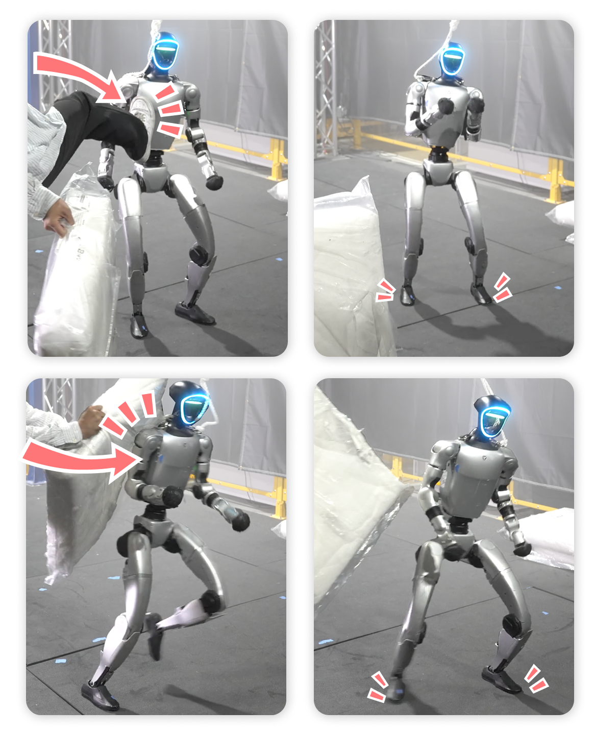
Booster T1 executes a learned locomotion controller, and Unitree G1 executes motion-tracking policies trained with the BeyondMimic protocol [4]. Six reference sequences cover dancing, walking, running, fighting motions, and jumping, with one policy per sequence and roughly two-and-a-half-minute average duration. Hardware sequences and perturbation examples demonstrate transfer using reduced integration steps. The paper does not report a large repeated hardware-trial success-rate study.
4.3 Manipulation Finetuning
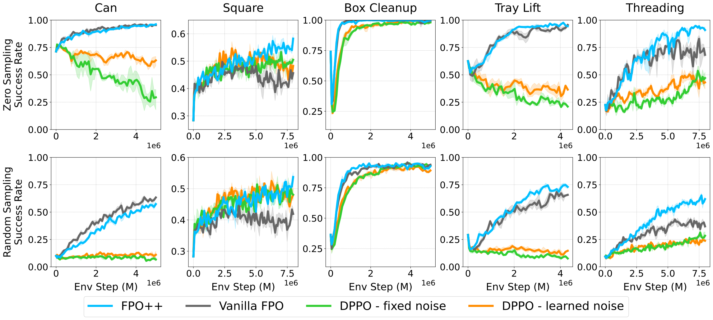
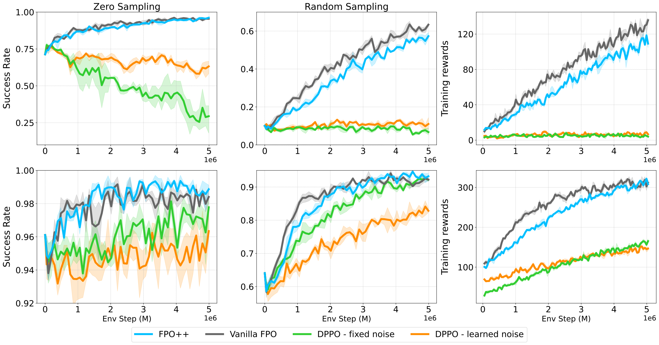
Five RoboMimic/DexMimicGen tasks use image-based demonstration pretraining followed by reward finetuning. Main comparisons initialize methods from the same base flow policy and include fixed-noise and learned-noise DPPO adaptations. Per-sample FPO++ with PPO clipping reaches strong success and generally learns faster. Vanilla FPO can also work well from a pretrained policy. Failures of the adapted DPPO variants depend strongly on exploratory base-policy quality and should be read alongside the original-code comparisons in the appendix.
4.4 Training Ablations
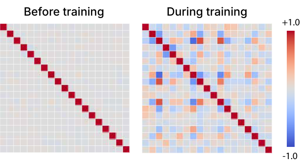
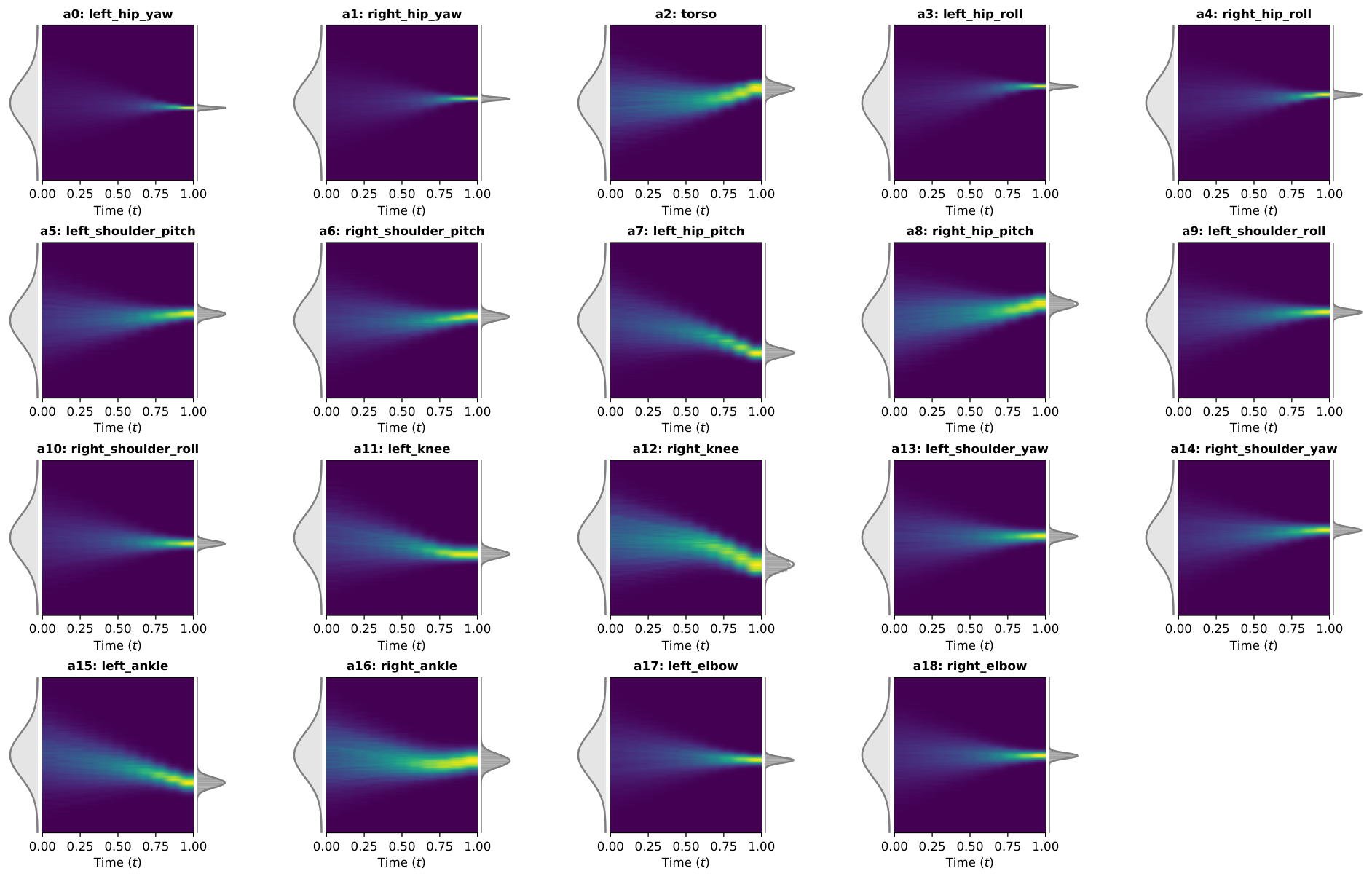
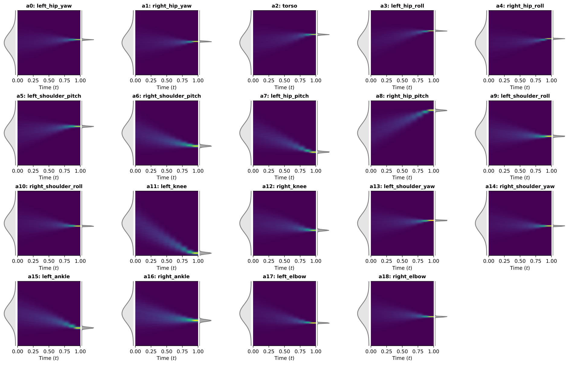
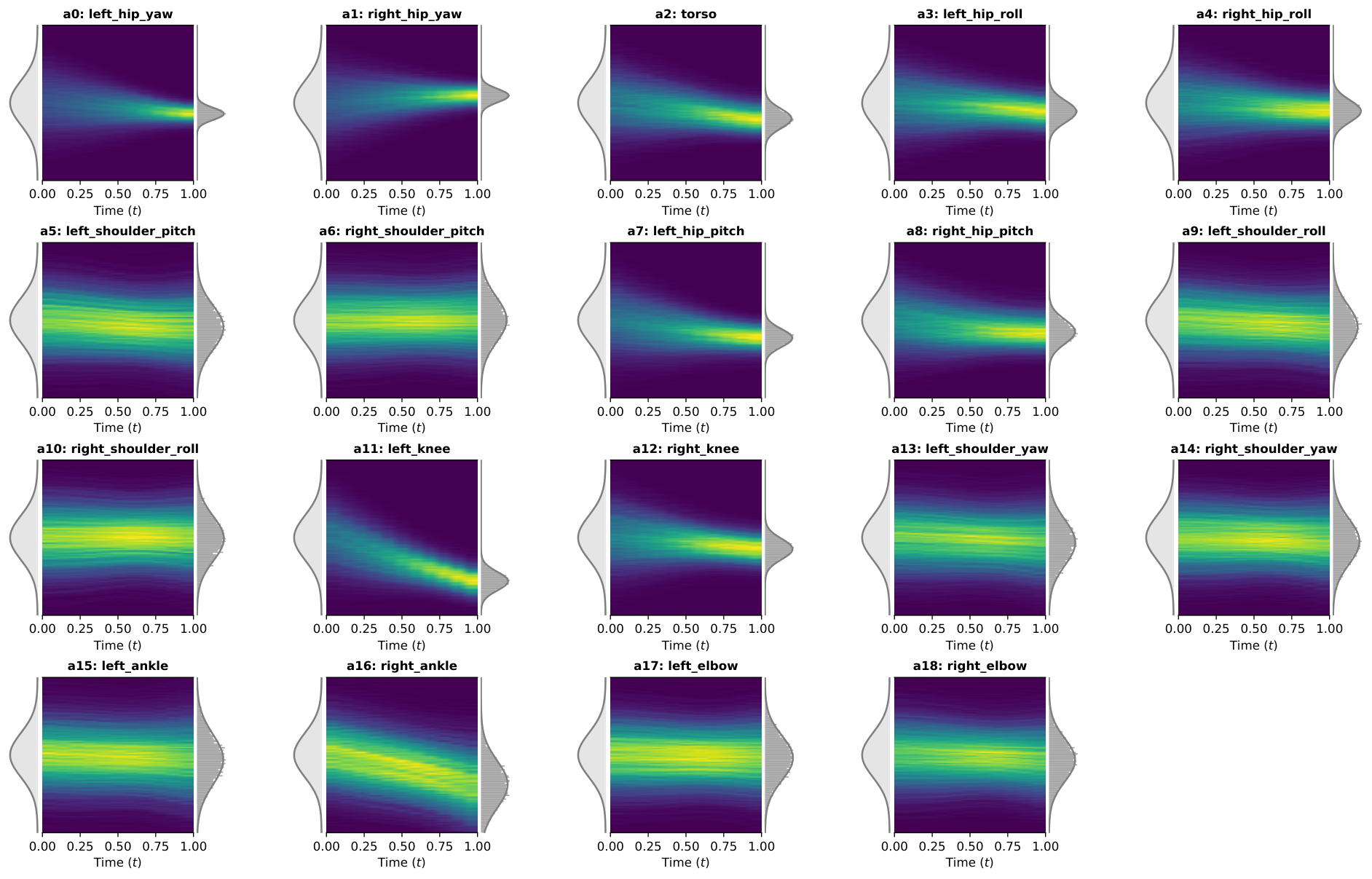
Locomotion ablations combine five seeds with several clip values. Removing per-sample ratios or replacing ASPO reduces average returns and increases variability. Gradient-alignment statistics and flow-field visualizations are consistent with more stable updates and broader action distributions.
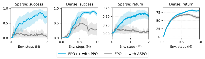
ASPO is not uniformly beneficial. With randomly initialized Lift action networks and a frozen pretrained visual encoder, sparse-reward final success is 0.07 for ASPO versus 0.73 for PPO; dense-reward success is 0.28 versus 0.81. Dense ASPO learns to grasp and hover for shaping reward without completing the task. These ten-seed tests implicate reward structure, not simply whether the action policy was pretrained. The paper recommends ASPO for well-aligned dense rewards and PPO clipping for sparse or exploitable shaping regimes.
4.5 Comparison with Gaussian PPO
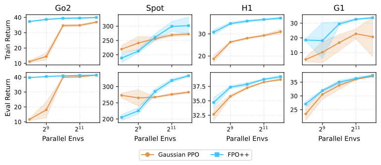
Across varied parallel-environment counts, FPO++ usually reaches stronger locomotion returns than the tested Gaussian PPO configurations. At a fixed observation, ten thousand sampled actions reveal learned cross-joint correlations, which a diagonal Gaussian cannot represent. Different algorithms also produce different gaits under the same task rewards; Spot’s rewards already include gait-coordination terms, so these are not wholly unshaped gait discoveries.
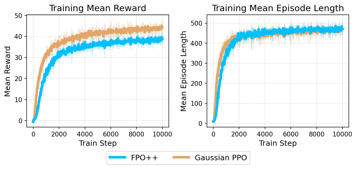
Tuned Gaussian PPO achieves higher motion-tracking returns when entropy regularization and adaptive learning rates are enabled. On an L40S, G1 locomotion reaches return twenty-five in nineteen minutes for Gaussian PPO versus twenty-three for FPO++; motion tracking can take up to twice as long. Expressiveness and sample efficiency therefore do not imply wall-clock superiority or a universally preferable controller.
5 Conclusion
The work demonstrates practical likelihood-free surrogate updates for flow policies, including humanoid transfer and manipulation finetuning. Per-sample ratios are broadly useful in the tested settings; ASPO requires reward-aware configuration. Future work must reduce computational cost and improve flow-policy regularization/adaptation, especially where a tuned Gaussian baseline already suffices.
Acknowledgments
The acknowledgments thank David McAllister, Arthur Allshire, and Chungmin Kim for discussions.
Appendix A Further related work
Related offline methods use advantage-weighted regression, value-based objectives regularized by generative losses, entropy bonuses, one-step flow policies, score matching, or adjoint matching. These differ from the paper’s online on-policy setting and address distinct challenges in propagating value gradients through generative policies.
Appendix B Experiment Details
Implementation details specify robot embodiments, reward structures, networks, sampling, domain randomization, and manipulation controls. All robot/task figures and hyperparameter tables are retained.
B.1 Locomotion Benchmarking
The locomotion benchmark follows IsaacLab velocity-command tasks, with common training settings and robot-specific rewards. Baselines receive explicit clipping sweeps.
B.1.1 Hyperparameters
Locomotion actor and critic networks have three layers of 256 and 768 hidden units, respectively. Default training uses 4,096 environments and twenty-four steps between updates. Flow actions use sixty-four Euler steps and updates use sixteen Monte Carlo samples per action. Quadrupeds train for 1,500 updates and humanoids for 2,000. Reducing integration steps to eight or sixteen harms training stability; rollout inference is not the dominant training cost in these small-network settings.
B.1.2 Environments and Rewards
Shared rewards track planar velocity and yaw while rewarding foot air time and penalizing excessive motion changes. Robot-specific penalties cover torques, contacts, body motion, and posture. Spot explicitly rewards diagonal-foot coordination and clearance; humanoids include fall penalties and biped air-time terms. Differences in learned gaits therefore arise within specified reward shaping rather than an absence of gait incentives.
B.2 Motion Tracking
The G1 tracking controller has twenty-nine degrees of freedom and runs at fifty hertz, using a five-millisecond simulator timestep with four-step decimation. Rewards, observations, and termination follow the referenced tracking protocol.
| Hyperparameter category | Used value | Sweep range and notes |
|---|---|---|
| FPO++ | ||
| Flow integration steps | ||
| Network output | , denotes data | |
| Samples per action | ||
| Training | ||
| Learning rate | , , | |
| Weight decay / Adam betas | / | AdamW parameters |
| Clip parameter | ||
| Discount factor () | ||
| GAE lambda () | ||
| Learning epochs | for Go2, others | |
| Minibatches per update | ||
| Running observation normalization | Yes | |
| Hyperparameter category | Used value | Sweep range and notes |
|---|---|---|
| FPO++ | ||
| Flow integration steps | ||
| Network output | , denotes data | |
| Samples per action | ||
| Training | ||
| Learning rate | ||
| Weight decay / Adam betas | / | AdamW parameters |
| Clip parameter | ||
| Discount factor () | ||
| GAE lambda () | ||
| Learning epochs | ||
| Minibatches per update | ||
| Running observation normalization | Yes | |
B.2.1 Domain Randomization
Randomization varies friction, restitution, joint defaults, torso center of mass, initial pose, and command delay. Perturbations every two to three seconds vary translational and angular velocities. Command delay spans zero to two simulation steps, or zero to ten milliseconds. These specified perturbations support transfer, without establishing robustness to all contacts or hardware variation.
B.2.2 Training Hyperparameters
Tracking training uses 4,096 environments, ninety-six rollout steps per update, and three-layer actor/critic networks with 1,024/512/256 widths. Policies train with fifty flow steps but deploy using five steps and deterministic zero-noise initialization. T1 locomotion uses the locomotion benchmark settings rather than this larger tracking configuration.
B.2.3 CFM loss implementation details
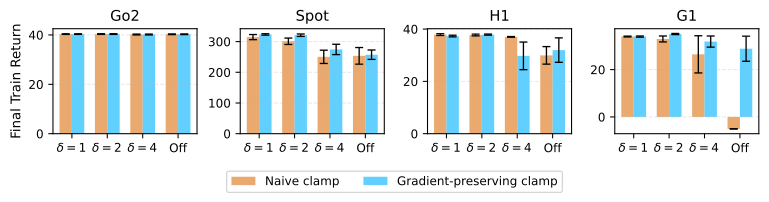
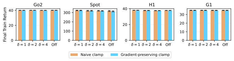
Exponentiating squared-loss differences can be unstable for large noise samples. The final implementation first clamps old and new conditional flow-matching losses, then clamps their difference before exponentiation. Experiments also test Huber losses and gradient-preserving clamping. These numerical safeguards are implementation details needed alongside the mathematical objective.
B.3 Manipulation finetuning
Manipulation uses actor/critic learning rates of 10⁻⁵/10⁻⁴ and advantage-estimation lambda 0.99. Discounts vary from 0.99 to 0.999 by task. Policies use ten flow steps, eight Monte Carlo samples per action chunk, and sixteen-step chunks, summing conditional-flow losses over chunk timesteps. Main DPPO variants adopt velocity prediction to share base policies and are tuned over clipping and exploration settings; they are adaptations, not identical copies of the original implementations.
Appendix C More experiments
Additional experiments examine environment scaling, emergent gaits, tracking baselines, original-code manipulation comparisons, base-policy sampling, and reward-dependent trust-region behavior.
C.1 Sample efficiency and emergent gaits versus Gaussian PPO
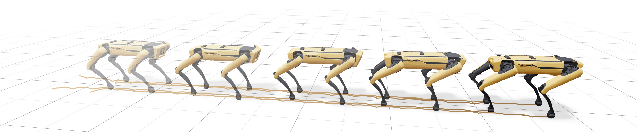
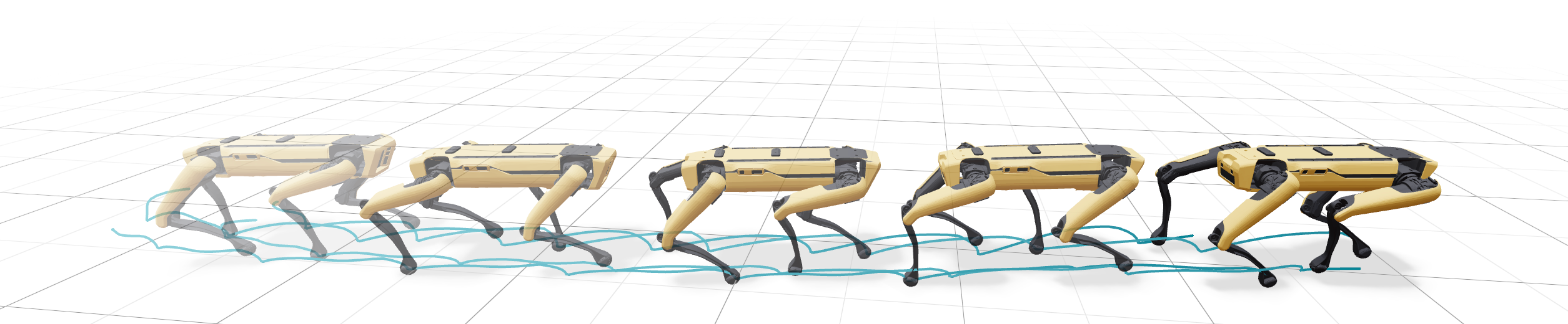
Locomotion comparisons sweep 256 through 4,096 parallel environments at fixed update counts, changing both minibatch size and total environment experience. Curves include five-seed dispersion. Gait examples compare controllers at the same one-meter-per-second command and reward definition.
C.2 Comparison with vanilla FPO for motion tracking
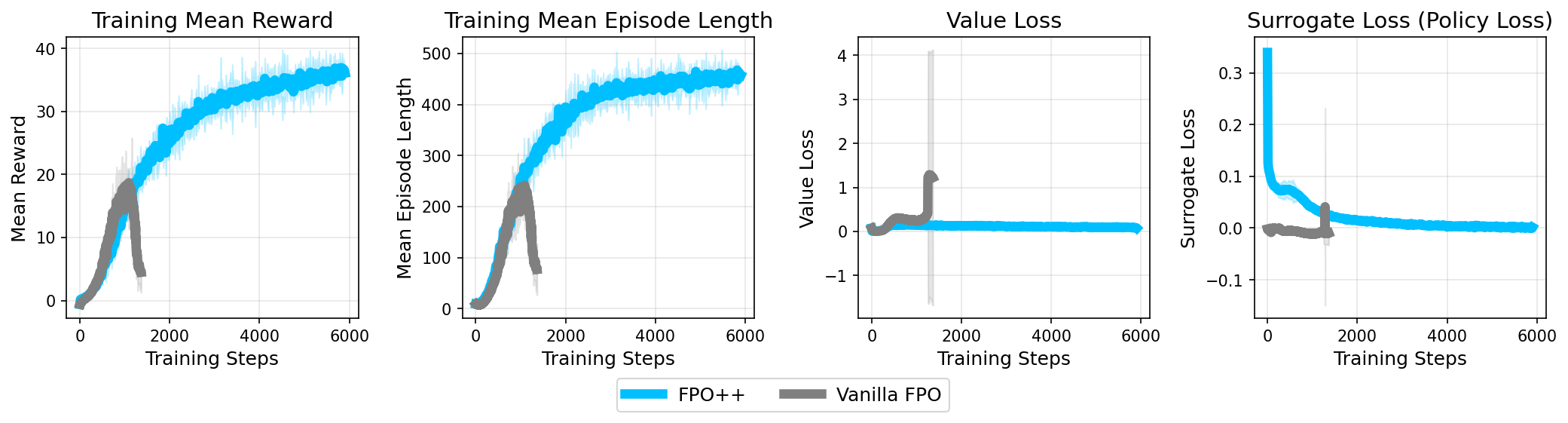
A motion-tracking comparison shows vanilla FPO improving initially, then collapsing with spikes in value and surrogate losses. FPO++ remains stable in the displayed training run and produces the deployed policy. This is a concrete instability example, not proof that every original-FPO configuration must fail.
C.3 Comparison with Gaussian PPO for motion tracking
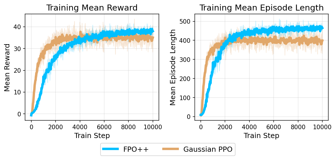
Without entropy bonuses or adaptive learning rates, FPO++ beats the simplified Gaussian tracking baseline. With both additions, Gaussian PPO attains higher return while episode lengths are similar. The experimental flow variant estimates entropy from nearest-neighbor action distances and adjusts learning rate using a noise-prediction-change statistic. That statistic is a heuristic policy-change proxy, not an exact KL divergence, and these additions are separate from the core objective.
C.4 Further comparisons with baselines in manipulation finetuning
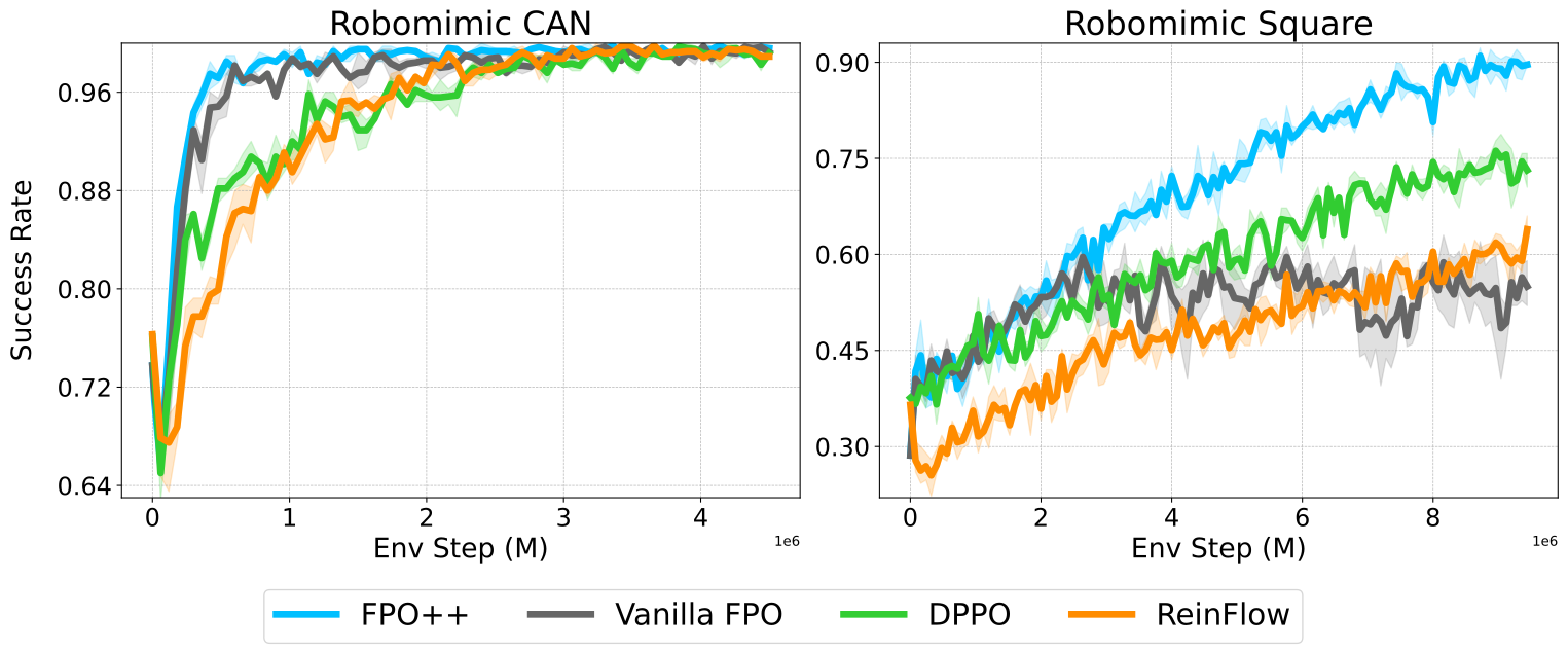
Original DPPO and ReinFlow code is compared under four-step chunks, with corresponding FPO variants trained in the adapted pipeline. These methods use different pretrained policies: Can starts near 74–76% success, while Square starts at 28.62% for FPO variants versus 36.50–37.60% for the alternatives. Original baselines use one hundred denoising/flow steps versus ten for FPO. FPO++ reaches the highest reported final success, but the comparison is not identical-base-policy evidence. Each checkpoint evaluates two hundred episodes across fifty environments.
C.5 Detailed analysis on the RoboMimic Can experiment
A Can base policy scores 71.35% with deterministic zero-sampling but only 10.00% with random initial noise. Low exploratory success produces few useful terminal rewards, and added denoising noise can worsen this. A stronger base policy scores 96.11%/64.36% under zero/random sampling, and DPPO variants then finetune successfully. This qualifies the main failure examples and separates deterministic evaluation quality from training exploration quality.
C.6 Ablation study for manipulation finetuning
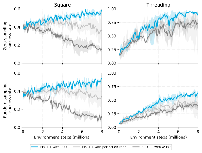
Square and Threading ablations average three training seeds and two hundred evaluation episodes per checkpoint per seed. Per-sample ratios with PPO clipping perform best. ASPO lowers final success despite its locomotion benefits, motivating the additional from-scratch reward tests.
C.7 ASPO under sparse and dense rewards
Lift comparisons use ten seeds, two million steps for sparse rewards or one million for dense rewards, and one hundred evaluation episodes per seed/checkpoint. Only action networks start randomly; the visual encoder remains pretrained and frozen. PPO clipping wins under both reward schemes even after separate tuning. Dense ASPO’s high shaping return alongside low completion demonstrates why return alone cannot establish task success.
Appendix D Analysis of training dynamics
Training-dynamics analysis examines gradient alignment, conditional action-distribution shape, and deterministic evaluation. These measurements help interpret empirical stability but do not establish convergence guarantees.
D.1 Empirical gradient variance
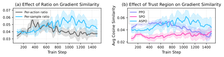
For each update, the analysis compares individual gradients with their mean using cosine similarity. Per-sample ratios and ASPO yield more aligned gradients, especially later in training. This supports a reduction in directional disagreement; cosine similarity is a proxy rather than a direct complete estimator of gradient variance.
D.2 Entropy and full-action-space flow fields
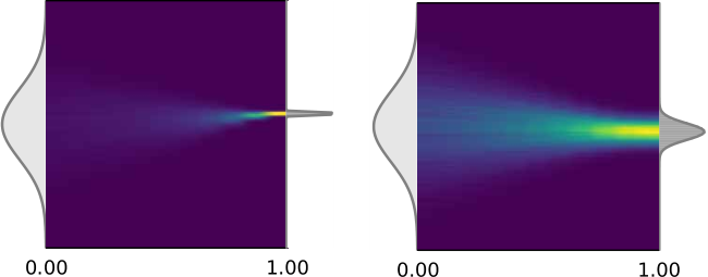
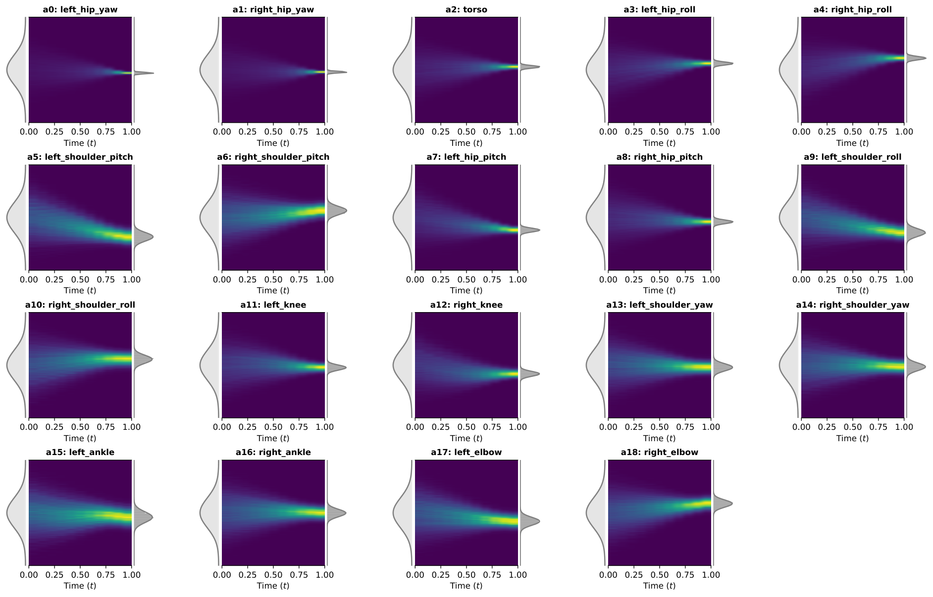
Flow trajectories for all nineteen H1 action dimensions show narrowing distributions during a PPO-clipped policy collapse and broader distributions for ASPO at intermediate and final checkpoints. Visualizations transport ten thousand initial noises with eight Euler steps, distinct from the sixty-four-step training rollouts. The retained single-joint and full-action-space panels show an association between distribution collapse and performance in these runs, not a universal entropy guarantee.
D.3 Zero-sampling
Zero-sampling starts flow integration at the zero vector instead of random Gaussian noise. It is a deterministic choice, not generally the mean action of a nonlinear flow distribution. For one perturbed two-and-a-half-minute tracking sequence over one hundred rollouts, zero-sampling returns are 45.1 with five steps and 45.5 with fifty, versus 34.7 and 38.4 for random sampling, with substantial reported dispersion. The small five-versus-fifty deterministic gap enables lower-latency hardware execution, while large random-versus-zero gaps explain why test success can exceed exploratory training success.
| Sampling method | 5 steps | 50 steps |
|---|---|---|
| Random sampling | ||
| Zero-sampling |