Overview
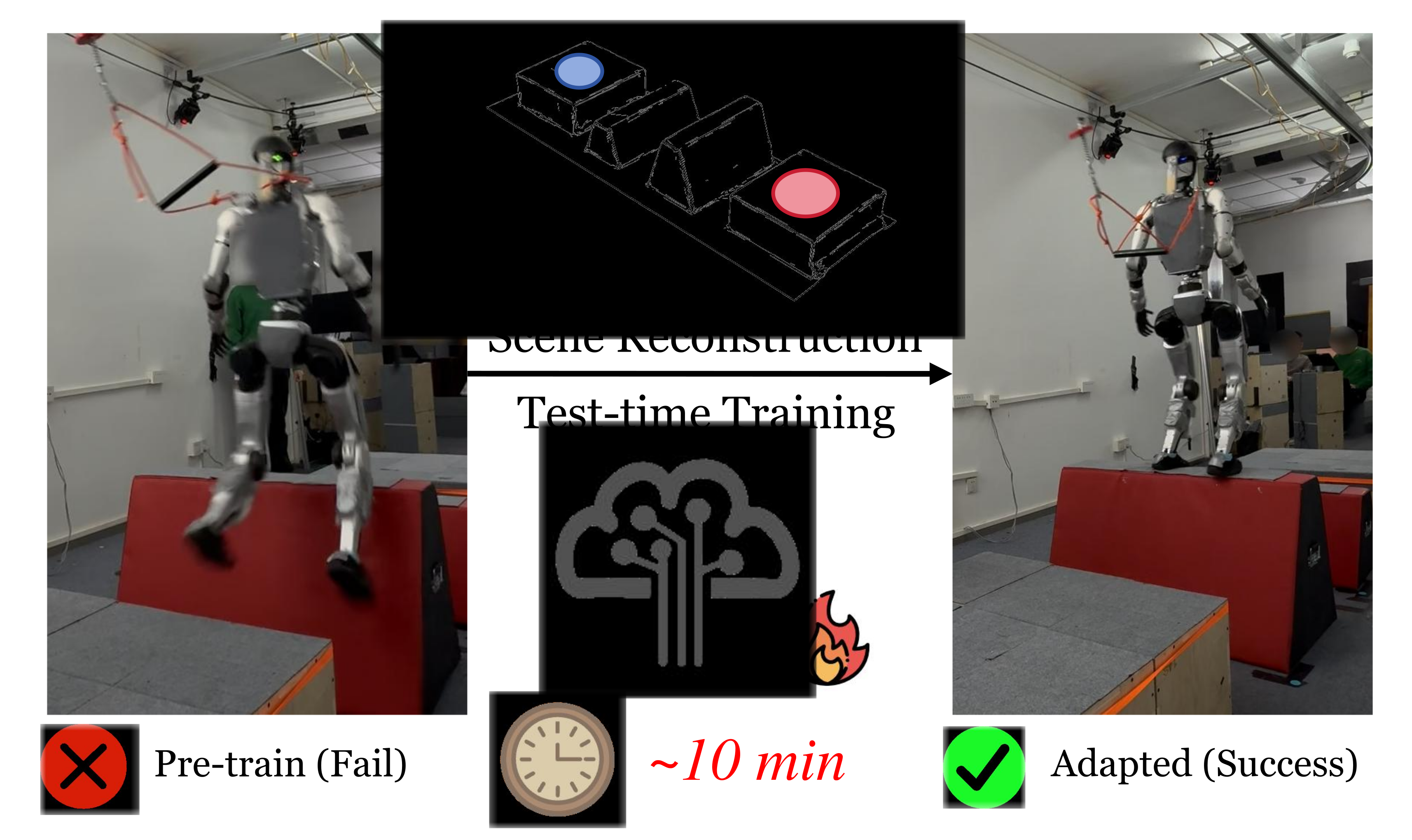
TTT-Parkour adapts a pretrained humanoid controller to a newly scanned obstacle course. Adaptation happens in a reconstructed simulator before physical execution, producing a specialist for that terrain.
At a glance
The pipeline combines handheld RGB-D capture, metric mesh reconstruction and short simulator fine-tuning. Across thirteen constructed courses, terrain-specific policies improve on the authors’ general pretrained controller. Ten courses reach the specified simulator threshold within 120 iterations; three take longer. The approximately ten-minute workflow excludes five days of pretraining, and hardware evaluation uses only five trials per course.
1 Introduction
Procedural pretraining may miss difficult real obstacle arrangements. Rather than enlarge the generalist indefinitely, scan the target course, reconstruct its collision geometry and adapt before deployment. Feed-forward visual reconstruction is fast but needs reliable scale and coordinate alignment for meaningful robot contacts.
This edition covers all 23 pages of arXiv v2, dated 13 October 2026, with all eight authors verified. The catalog retains the February preprint date. Test-time training here is offline workstation training for a specific environment, not gradient updates during a robot run or autonomous online exploration.
2 Related Work
The work combines perceptive locomotion, target-environment adaptation and simulation-ready reconstruction rather than introducing a wholly new locomotion learner.
2.1 Perceptive Locomotion
Map-based controllers depend on localization and reconstruction consistency; direct depth controllers use local visual evidence without a persistent map. The policy builds on the end-to-end depth/proprioception paradigm also used in Hiking in the Wild.
2.2 Fast Adaptation
Test-time methods can modify predictions, trajectories or model parameters. This approach updates policy parameters inside a reconstructed simulator before execution, complementing a general policy with an environment-specific specialist.
2.3 Scene Reconstruction
Radiance-field and Gaussian-splat methods emphasize appearance and may need extra processing for collision meshes. Feed-forward reconstruction avoids scene-specific optimization but can have scale/distortion errors. The proposed contribution is a fast metric reconstruction/alignment workflow suited to the tested narrow contact surfaces.
3 Method
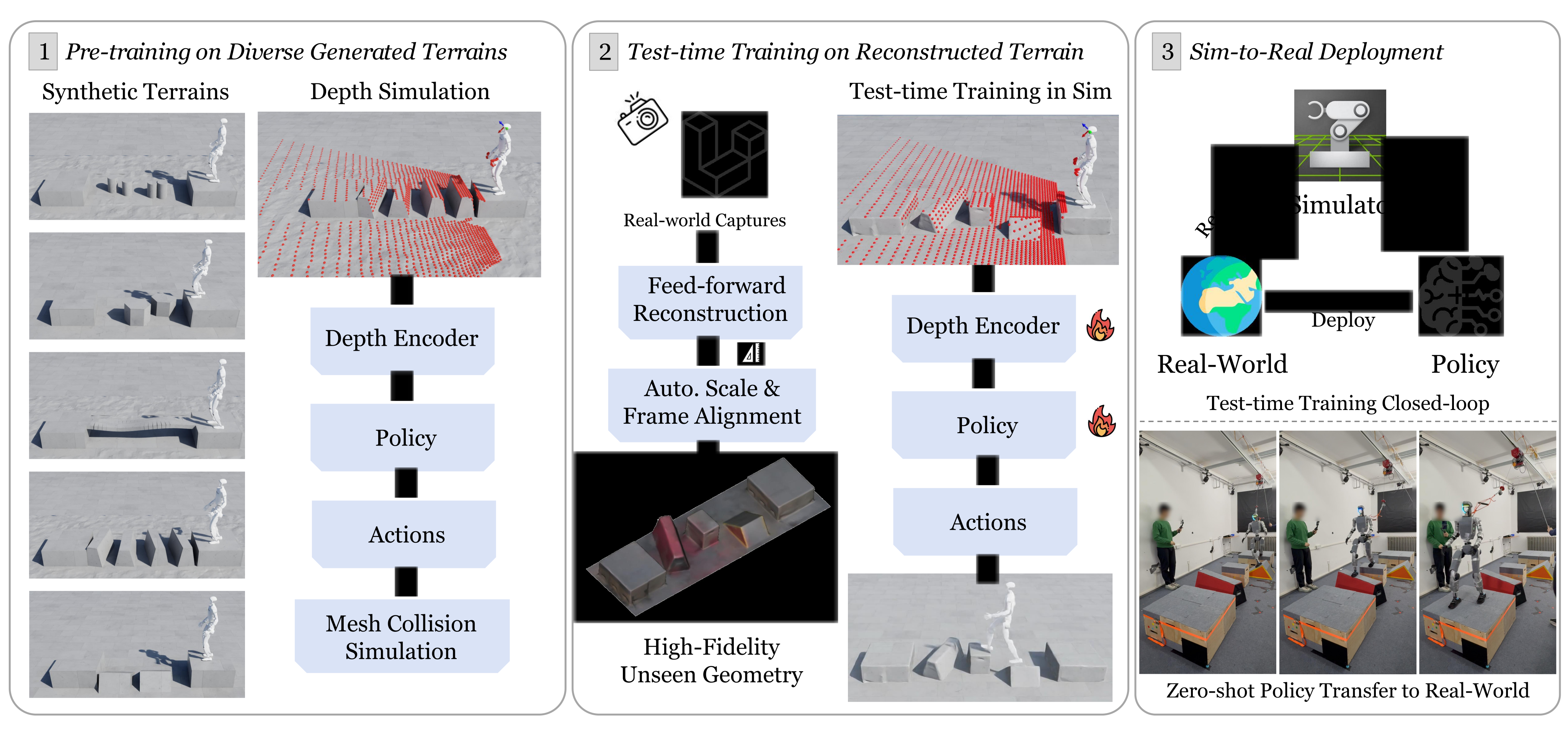
The three stages are broad policy pretraining, reconstruction plus target-course fine-tuning, and physical execution without further policy updates.
3.1 Problem Definition
Traverse elevated platforms from a start to an end platform using only feet and legged motion. Ground contact is failure, preventing shortcuts around obstacles. Trials use a fixed forward velocity command and zero commanded yaw; they do not test arbitrary navigation directions or hand-assisted climbing.
3.2 Policy Pre-training
PPO trains an asymmetric actor–critic from noisy proprioceptive history and strided depth history. A CNN and MLP embed depth, then a mixture-of-experts policy outputs 29 joint-position targets for PD control. The critic receives clean state and base linear velocity. Task, edge/contact, regularization, safety and AMP rewards shape the policy.
3.3 Efficient Geometry Reconstruction
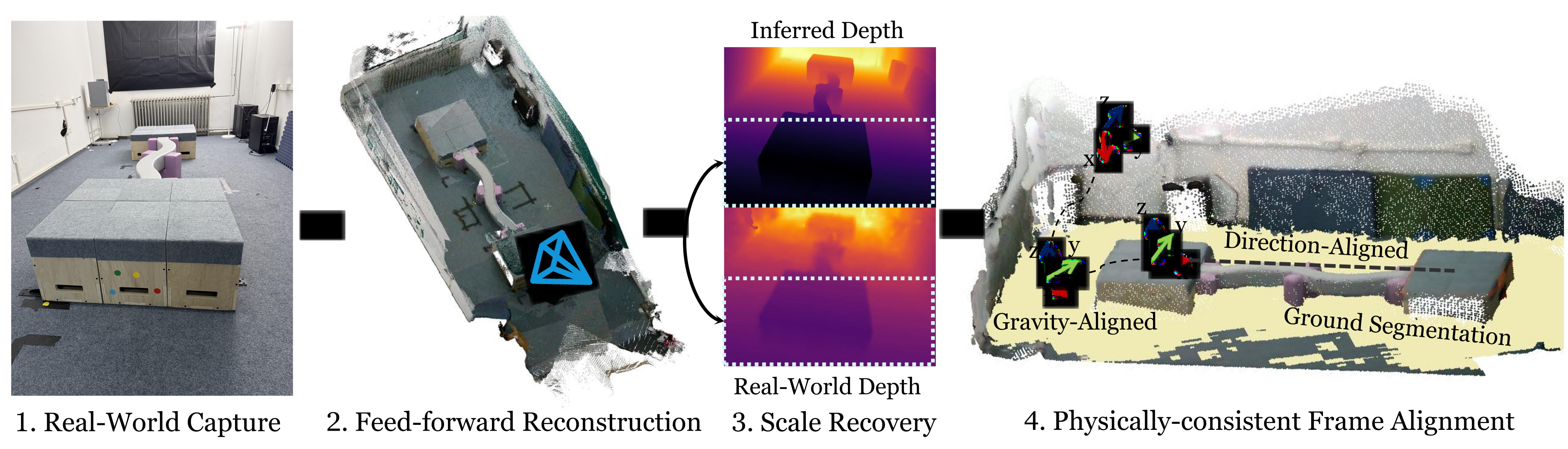
Geometry: π³ predicts a scale-ambiguous point cloud from RGB frames, and Screened Poisson reconstruction produces a mesh. Scale: use the ratio of median predicted and sensor depth in the image’s lower half, favoring terrain over distant background. This makes residual scale error small enough for ordinary randomization in the tested cases.
Frame: segment ground, reject outliers with RANSAC, and estimate its normal with PCA. Align that normal to vertical, set the origin at the start-platform centroid, and align the start-to-end vector with simulator x. The procedure assumes a ground plane orthogonal to gravity and identifiable start/end platforms. It does not establish correct alignment for arbitrary sloped ground or missing/incorrect segmentation.
3.4 Rapid Test-Time Policy Training
Fine-tune on one reconstructed target terrain while preserving observation/action interfaces and rewards. Compare updating all weights against frozen-base adapters, additive residual actions and final-actor-layer-only training. No additional physical policy learning occurs after simulator adaptation.
4 Experiments
Experiments separate adaptation quality, reconstruction fidelity/speed, convergence and cross-terrain transfer. Strong target-course performance is not equivalent to retaining broad generalist competence.
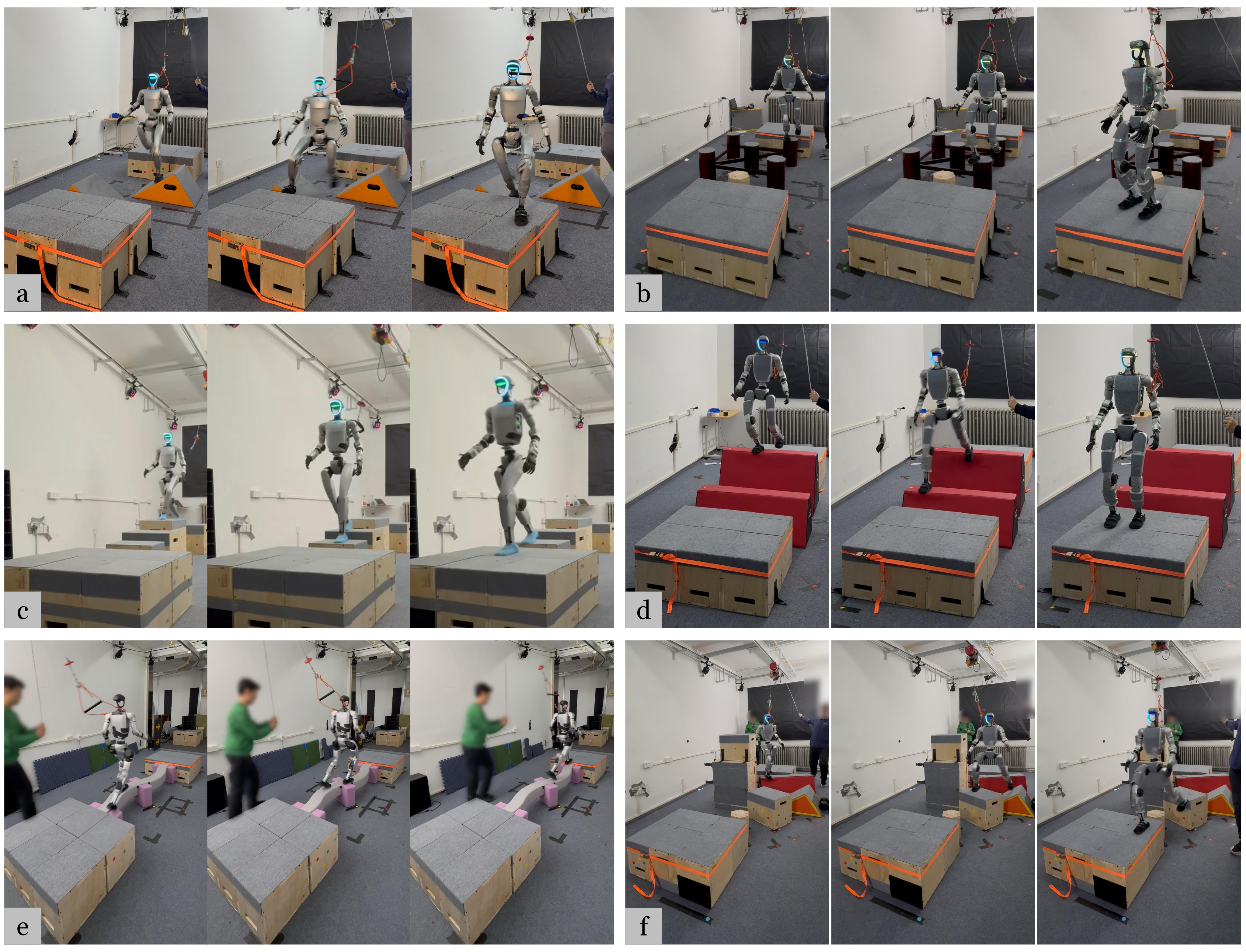
4.1 Experiment Configuration
Use 4,096 parallel G1 agents on one RTX 5090, reported at under four seconds per iteration. Pretraining takes approximately five days. Thirteen hardware courses receive five trials each; simulation success reports three evaluation seeds with 1,000 trials per course per seed. Those seeds measure evaluation variation of trained policies, not independent training-run variability.
4.2 Traversability Analysis
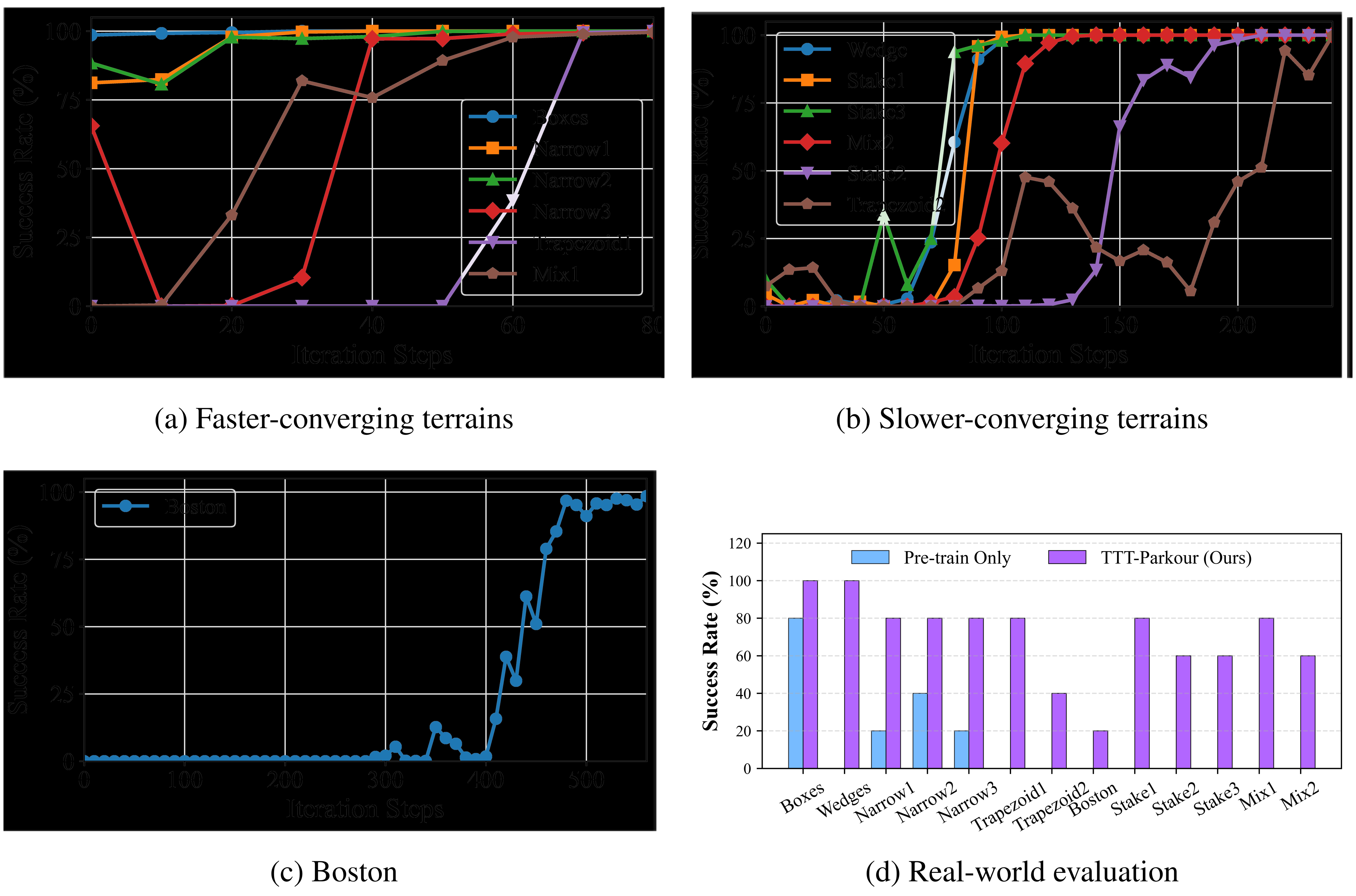
Compare the pretrained base, single-course scratch training, joint scratch training on thirteen courses, joint fine-tuning (TTT-13) and single-course fine-tuning (TTT-1). Converged TTT-13/TTT-1 average 99.56%/99.83% simulated success. Joint fine-tuning needs 1,500 iterations; target-course adaptation crosses 97% within 560 on every course. Scratch-13 remains at zero after 30,000 iterations under this setup.
Ten courses cross 97% within 120 iterations; Stake2, Trapezoid2 and Boston need 200, 240 and 560. Capture/reconstruction is 2 minutes 10 seconds, with about eight minutes fine-tuning for most courses. The ten-minute headline is therefore neither an all-course maximum nor the total cost including pretraining.
Hardware Figure 5d gives 5/5 for Boxes/Wedges; 4/5 for Narrow1–3, Trapezoid1, Stake1 and Mix1; 3/5 for Stake2/3 and Mix2; 2/5 for Trapezoid2; and 1/5 for Boston. The base succeeds on Boxes (4/5), Narrow1/3 (1/5) and Narrow2 (2/5), with zero elsewhere. The low Boston/Trapezoid2 counts temper the near-perfect simulator results.
Most scalar dimensions overlap pretraining, while shape, placement and obstacle combinations differ. These tests establish improvement over this base controller, not over every stronger generalist. Wobbling physical obstacles, camera/actuator differences and residual geometric error are proposed sources of the simulation-to-hardware gap.
| Terrain | Pre-train | Scratch-1 | Scratch-13 | TTT-13 | TTT-1 |
|---|---|---|---|---|---|
| (25k) | (30k) | (1.5k) | (Converged) | ||
| Boxes | 98.27±0.21% | 0.00±0.00% | 0.00±0.00% | 98.80±0.46% | 100.00±0.00% |
| Wedges | 0.30±0.30% | 0.00±0.00% | 0.00±0.00% | 99.93±0.12% | 99.90±0.00% |
| Nar.1 | 82.70±0.70% | 100.00±0.00% | 0.00±0.00% | 99.53±0.21% | 99.97±0.06% |
| Nar.2 | 87.27±1.24% | 100.00±0.00% | 0.00±0.00% | 100.00±0.00% | 99.97±0.06% |
| Nar.3 | 71.63±4.08% | 0.23±0.12% | 0.00±0.00% | 99.20±0.17% | 99.37±0.15% |
| Trap.1 | 0.00±0.00% | 0.00±0.00% | 0.00±0.00% | 100.00±0.00% | 99.97±0.06% |
| Trap.2 | 7.27±1.21% | 0.00±0.00% | 0.00±0.00% | 99.57±0.15% | 99.93±0.06% |
| Boston | 0.00±0.00% | 0.00±0.00% | 0.00±0.00% | 98.93±0.50% | 99.20±0.00% |
| Stake1 | 3.67±0.40% | 0.00±0.00% | 0.00±0.00% | 100.00±0.00% | 99.97±0.06% |
| Stake2 | 0.17±0.06% | 0.00±0.00% | 0.00±0.00% | 99.00±0.17% | 99.93±0.06% |
| Stake3 | 9.63±1.32% | 0.00±0.00% | 0.00±0.00% | 99.90±0.17% | 99.80±0.17% |
| Mix1 | 0.07±0.06% | 0.00±0.00% | 0.00±0.00% | 100.00±0.00% | 99.77±0.23% |
| Mix2 | 0.00±0.00% | 0.00±0.00% | 0.00±0.00% | 99.43±0.25% | 100.00±0.00% |
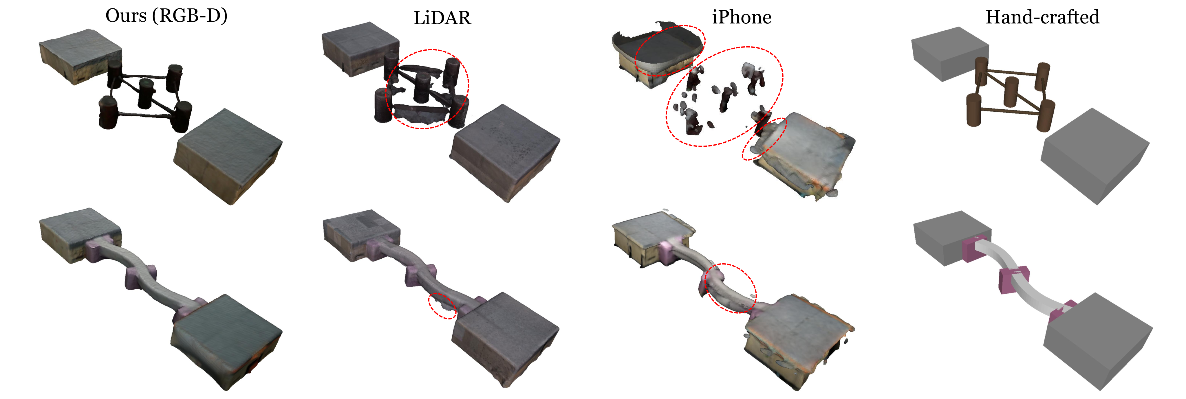
| Methods | RGB-D | LiDAR Scanner | iPhone | Hand-crafted |
|---|---|---|---|---|
| Pros | Balanced quality and efficiency | Professional, best scale accuracy | Most accessible, fast acquisition | No artifacts |
| Cons | Scale precision slightly lower than LiDAR | Terrain junction artifacts, tedious post-processing | Unstable reconstruction results, flying point artifacts | High manual effort, over-perfect geometry causes sim-to-real gap |
| Time | 2 min 10 s | 20 min | 4 min | 1 h |
4.3 Mesh Reconstruction Analysis
RGB-D reconstruction takes 2:10 versus LiDAR 20 minutes, iPhone four minutes and hand construction one hour in Table 2. RGB-D absolute relative scale errors range from 0.2% to 2.8% on the four evaluated courses; LiDAR is comparable, while RGB-only baselines have much larger scale errors.
Hardware reconstruction comparisons use five trials per condition. RGB-D and LiDAR are competitive; iPhone artifacts and idealized hand meshes transfer less reliably. Scale/shape metrics register to a hand-measured reference, which itself omits some real irregularities. Local geometric error and transfer are associated in these examples, without a controlled causal perturbation study.
4.4 Convergence Analysis
Only two narrow-beam scratch policies reach 97% by about 17,000 iterations; most remain below threshold after 25,000. TTT-1 specializes much faster than scratch training and usually faster than TTT-13. Joint batches devote fewer samples to each course, a plausible explanation not isolated by a matched-per-course-sample ablation. Trapezoid2 benefits from joint training in the reported comparison.
5 Conclusion and Limitations
The system provides useful on-demand specialists but requires manual capture and a separate workstation. The fixed onboard camera cannot autonomously scan a complete course. Transfer to unrelated terrain is limited, stronger-generalist comparisons and controlled geometry perturbations remain untested, and five physical trials per condition provide limited precision. Saving the original checkpoint does not demonstrate that a fine-tuned policy retains its old abilities.
Acknowledgments
The project acknowledges support from Tsinghua University’s Initiative Scientific Research Program.
Appendix
The appendices retain complete training/reward settings, reconstruction and convergence tables, adaptation variants, all course dimensions and the full transfer matrix.
| A | Policy Pre-training Details .A |
| B | Mesh Reconstruction Analysis .B |
| C | Convergence Analysis .C |
| D | Test-Time Training Strategies .D |
| E | Experiment Configuration .E |
| F | Geometric Specifications of Real-World Terrains .F |
| G | Cross-Terrain Transfer .G |
Appendix A Policy Pre-training Details
Pretraining uses a 20-column by 10-row grid: five terrain families occupy four columns each, with increasing difficulty over rows.
A.1 Observations, Actions, and Terminations
The actor observes angular velocity, projected gravity, commands, joint positions/velocities, previous actions and depth history. It outputs 29 position targets; the critic additionally sees base linear velocity. Eight proprioceptive steps are used. Yaw commands remain zero for parkour despite the interface supporting yaw.
Terminate on timeout, remaining at the start over four seconds, any body link touching the ground, or excessive base orientation. Numerical timeout/tilt and several noise/history parameters are not fully supplied in the manuscript.
| Space | Signal | Dim | Description |
|---|---|---|---|
| Actor Obs | Base Angular Velocity | 3 | IMU gyroscope |
| Projected Gravity | 3 | Gravity direction in base frame | |
| Velocity Commands | 3 | ||
| Joint Positions | 29 | 29-DoF joint angles | |
| Joint Velocities | 29 | 29-DoF joint velocities | |
| Last Action | 29 | Previous target joint positions | |
| Depth History | Strided depth frames (32×18 each) | ||
| Critic Obs | + Base Linear Velocity | 3 | Noise-free; critic only |
| Action | Target Joint Positions | 29 | Executed via PD control: |
A.2 Policy Network
A CNN maps depth through two 256-unit projections into 128 features. The MoE has four experts, a 256-unit gate and expert widths 256/128/64 with ELU; the AMP discriminator has widths 1024/512. Table 6 retains the exact stated network settings.
| Parameter | Value |
|---|---|
| CNN channels | [4] |
| CNN kernel sizes | [3] |
| CNN strides | [1] |
| CNN paddings | [1] |
| CNN pooling | MaxPool |
| Encoder projection units | [256, 256] |
| Encoder embedding dim | 128 |
| Encoder activation | ReLU |
| Policy Type | MoE |
| Number of Experts | 4 |
| Gating hidden units | [256] |
| Expert hidden units | [256, 128, 64] |
| Policy activation | ELU |
| Discriminator hidden units | [1024, 512] |
| Discriminator activation | ReLU |
A.3 AMP and Rewards
The AMP reference contains 57,979 MPC-generated frames at 50 Hz, approximately 1,159.6 seconds. Commands change every five seconds, spanning forward 0–1 m/s, lateral ±0.3 m/s and yaw ±1 rad/s during reference collection, distinct from fixed-forward parkour evaluation.
Pretraining and adaptation use the same full reward table. Notable weights are linear tracking +2, angular tracking +0.1, edge penetration −1, foot distance +1 and AMP +0.25. A sequence discriminator uses least-squares reference/policy targets and a clipped quadratic style reward (Equations 1–2). The appendix describes goal-derived training tracking, whereas physical evaluation uses constant forward speed and zero yaw; those contexts should not be conflated.
Equations 1–2
| (1) |
| (2) |
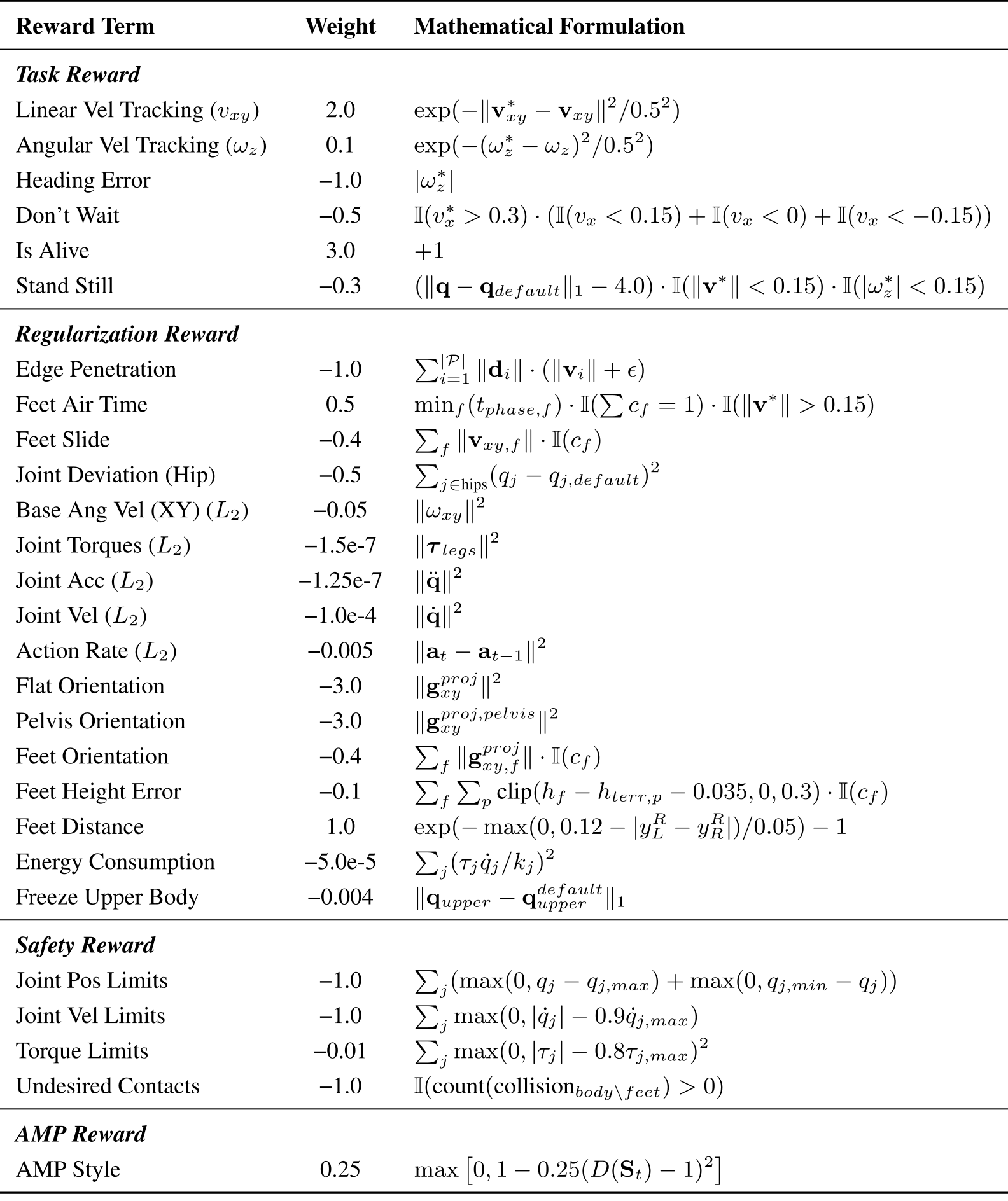
Original selectable source
| Reward Term | Weight | Mathematical Formulation |
| Task Reward | ||
| Linear Vel Tracking () | 2.0 | |
| Angular Vel Tracking () | 0.1 | |
| Heading Error | −1.0 | |
| Don’t Wait | −0.5 | |
| Is Alive | 3.0 | |
| Stand Still | −0.3 | |
| Regularization Reward | ||
| Edge Penetration | −1.0 | |
| Feet Air Time | 0.5 | |
| Feet Slide | −0.4 | |
| Joint Deviation (Hip) | −0.5 | |
| Base Ang Vel (XY) () | −0.05 | |
| Joint Torques () | −1.5e-7 | |
| Joint Acc () | −1.25e-7 | |
| Joint Vel () | −1.0e-4 | |
| Action Rate () | −0.005 | |
| Flat Orientation | −3.0 | |
| Pelvis Orientation | −3.0 | |
| Feet Orientation | −0.4 | |
| Feet Height Error | −0.1 | |
| Feet Distance | 1.0 | |
| Energy Consumption | −5.0e-5 | |
| Freeze Upper Body | −0.004 | |
| Safety Reward | ||
| Joint Pos Limits | −1.0 | |
| Joint Vel Limits | −1.0 | |
| Torque Limits | −0.01 | |
| Undesired Contacts | −1.0 | |
| AMP Reward | ||
| AMP Style | 0.25 | |
Appendix B Mesh Reconstruction Analysis
Compare D435i RGB-D, Lixel K1 LiDAR, iPhone 16 Pro with 3D Scanner App, and manually measured Trimesh geometry. LiDAR needs mapping/cleanup; iPhone meshes can contain flying artifacts; hand-built geometry misses physical irregularities. These specific workflows, sensors and courses delimit the timing/quality comparison.
Table 8 preserves Chamfer distance and 95th-percentile Hausdorff error. On Trapezoid1, RGB-D/LiDAR have similar global distance (0.029/0.031 m), but local error differs (0.036/0.080 m) alongside hardware success (4/5 versus 3/5). This supports examining local contact geometry, without proving which error alone caused each failure.
| Terrain | RGB-D | LiDAR | iPhone | MapAnything | Pi3 |
|---|---|---|---|---|---|
| Stake1 | 0.050/0.078 | 0.055/0.149 | 0.115/0.194 | 0.115/0.227 | 0.195/0.343 |
| Narrow1 | 0.052/0.076 | 0.047/0.071 | 0.135/0.232 | 0.115/0.187 | 0.211/0.379 |
| Wedge | 0.029/0.036 | 0.045/0.057 | 0.048/0.067 | 0.198/0.344 | 0.236/0.396 |
| Trapezoid1 | 0.029/0.036 | 0.031/0.080 | 0.151/0.247 | 0.210/0.353 | 0.209/0.356 |
Appendix C Convergence Analysis
Table 9 measures the first crossing of 97% simulated success, not the time required to establish hardware reliability. Boxes already exceed that threshold at zero adaptation steps. TTT-13’s Boston entry remains “>1000” from an earlier window, while its extended 1,500-step result is 98.93%; these are compatible, different stopping summaries.
For Trapezoid2, joint fine-tuning reaches threshold at 170 steps versus 240 for single-course adaptation. Transfer from similar beam geometry is a hypothesis. The 1,500-step joint controller also covers all thirteen targets simultaneously, unlike thirteen separate specialists.
| Terrain | Scratch-1 | TTT-13 | TTT-1 |
|---|---|---|---|
| Boxes | >25k | 0 | 0 |
| Wedges | >25k | 250 | 100 |
| Nar.1 | 17k | 70 | 20 |
| Nar.2 | 17k | 70 | 20 |
| Nar.3 | >25k | 70 | 40 |
| Trap.1 | >25k | 230 | 70 |
| Trap.2 | >25k | 170 | 240 |
| Boston | >25k | >1000 | 560 |
| Stake1 | >25k | 350 | 100 |
| Stake2 | >25k | 400 | 200 |
| Stake3 | >25k | 260 | 100 |
| Mix1 | >25k | 160 | 60 |
| Mix2 | >25k | 270 | 120 |
Appendix D Test-Time Training Strategies
Full fine-tuning updates the pretrained network; adapters learn new feature corrections with frozen original weights; residual learning adds a separately initialized action correction; last-layer training changes only the final actor layer. Zero output initialization preserves the starting behavior for adapter/residual variants.
Table 10 favors full fine-tuning on Narrow1 (20 iterations versus 40/40/120) and Mix2 (120 versus 200/>1000/260). On Trapezoid1, however, full/residual take 70 while last-layer/adapter take 60. Thus the prose’s claim that parameter-efficient methods consistently underperform is too broad. Simulation is said to dominate runtime, but detailed timing/memory measurements for these variants are not supplied.
| Terrains / Methods | Last Layer | Residual | Adapter | Full Fine-tuning (Ours) |
|---|---|---|---|---|
| Narrow1 | 120 | 40 | 40 | 20 |
| Trapezoid1 | 60 | 70 | 60 | 70 |
| Mix2 | 200 | >1000 | 260 | 120 |
Appendix E Experiment Configuration
Training and deployment use the same robot interface, with separate workstation adaptation and onboard execution.
E.1 Training Setup
IsaacLab/IsaacSim simulate 4,096 29-DOF G1 agents on an RTX 5090. Pretrain for 100,000 iterations; use Warp ray-cast depth and eight-step proprioceptive history. These substantial initial training costs are amortized before the short target-course adaptation phase.
E.2 Policy Deployment on Real Robot
Deploy through ROS2 on a Jetson Orin NX at 50 Hz, with D435i depth at 60 Hz. Downsample 480×270 images to 64×36 and crop a center-bottom 32×18 patch. The adapted policy receives no further physical parameter updates.
E.3 Tested Terrains
Start/end boxes are approximately 0.90×0.80×0.35 m. Training covers five families and 200 curriculum configurations; real evaluation constructs thirteen arrangements. Table 11 shows overlapping dimension ranges but irregular shapes, cross-family mixtures and Boston’s multilevel topology. This is a coverage description, not a quantified distribution-distance test.
| Terrain | Pre-training | Real-world test |
|---|---|---|
| Boxes | Size 0.30–0.82; height 0.30–0.50; gap 0.35 | Height 0.40–0.50; gap 0.31–0.32 |
| Wedges | Size 0.15–0.82; height 0.13–0.35; slope /60∘ | Height 0.31; slope 30∘ |
| Narrow | Span 1.43–2.63; width 0.15–0.60; height 0.25–0.45; curved | Length 2.0; width 0.14–0.27; height 0.32–0.48; irregularly curved |
| Stakes | Diameter 0.16–0.24; height 0.30–0.45; 5–7 piles | Diameter 0.18; height 0.40; irregular layouts |
| Trapezoids | Top length 0.135–0.275; width 0.81–0.89; height 0.15–0.55 | Width up to 1.0; height 0.35–0.55 |
| Mix1/2 | Single terrain family per training terrain | Cross-family obstacle compositions |
| Boston | No direct counterpart | Irregular multi-level topology |
E.4 Evaluation Metrics
Initialize on the start platform and command constant forward speed with zero yaw. Success means reaching the end without touching the ground or falling. Physical conditions use five trials; simulation uses 1,000 per cell per evaluation seed and three seeds. Initial position and some heading randomization test limited route variation, not changed obstacle geometry or unrestricted directional control.
Appendix F Geometric Specifications of Real-World Terrains
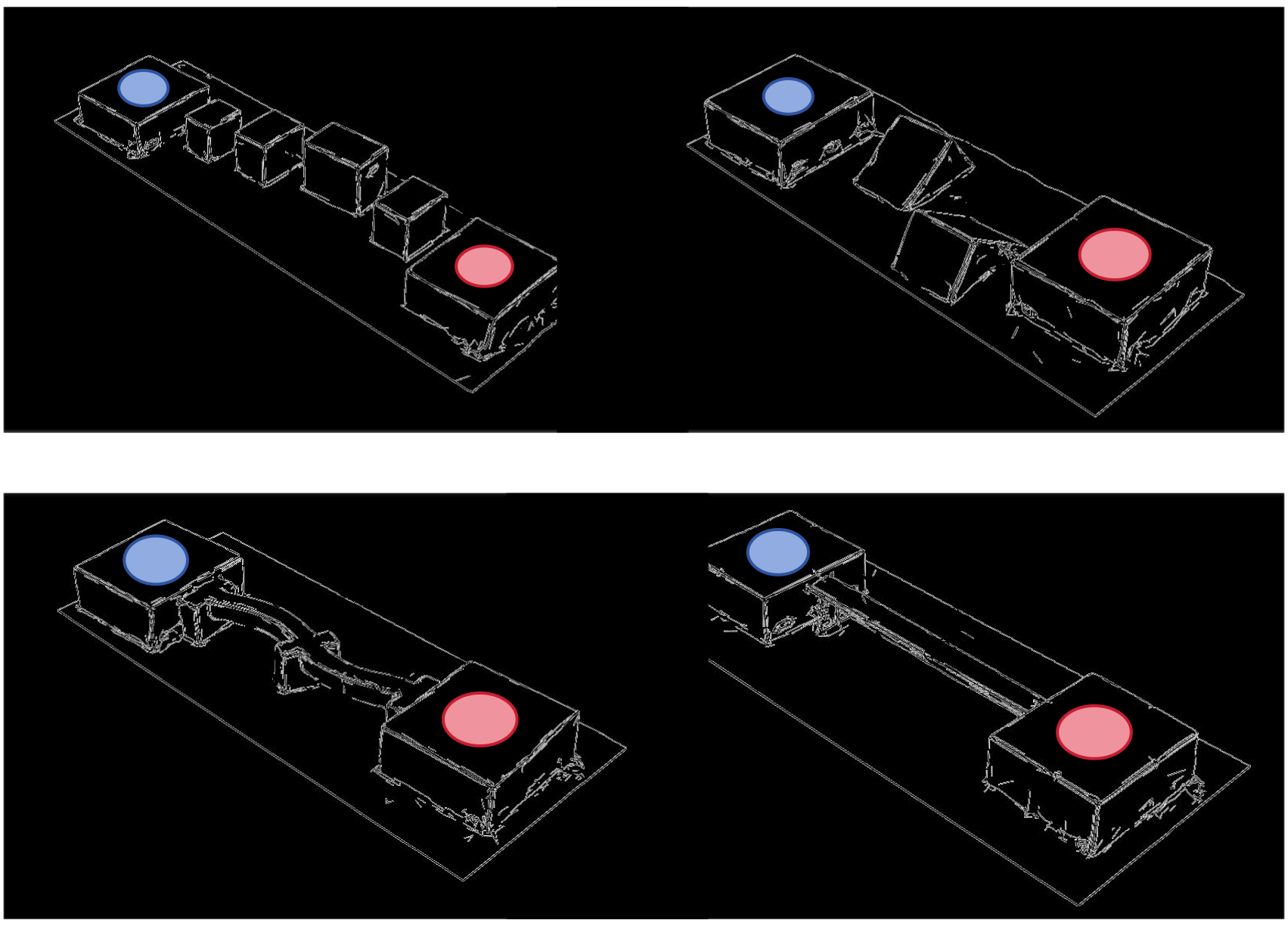
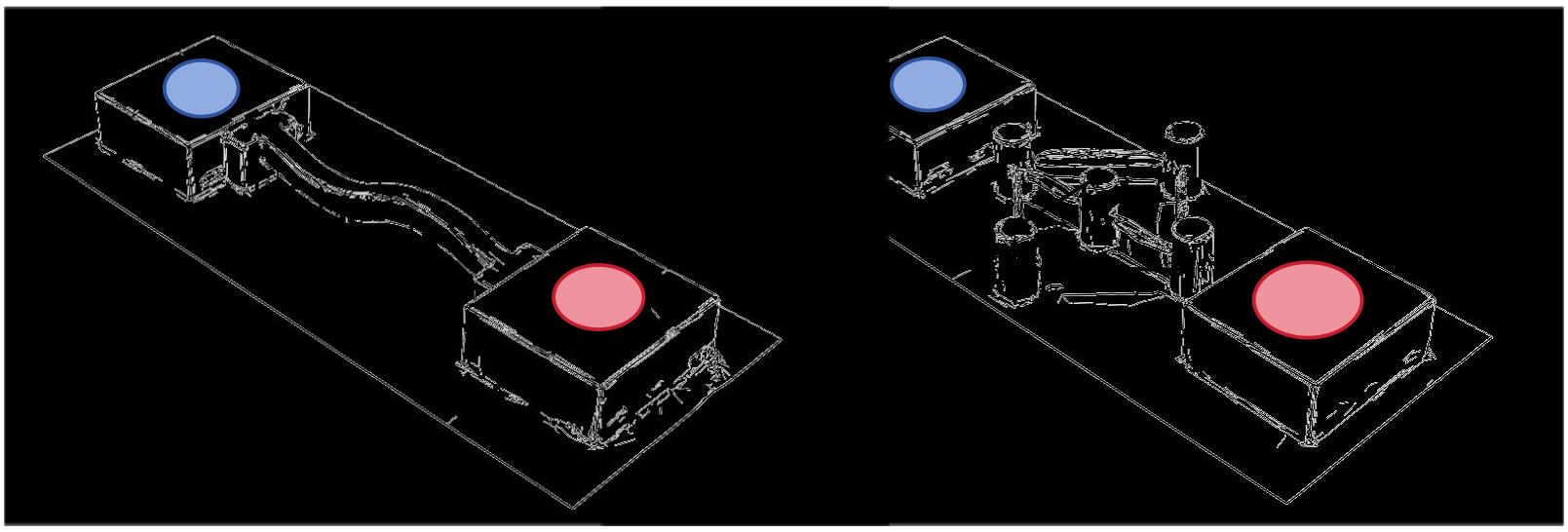
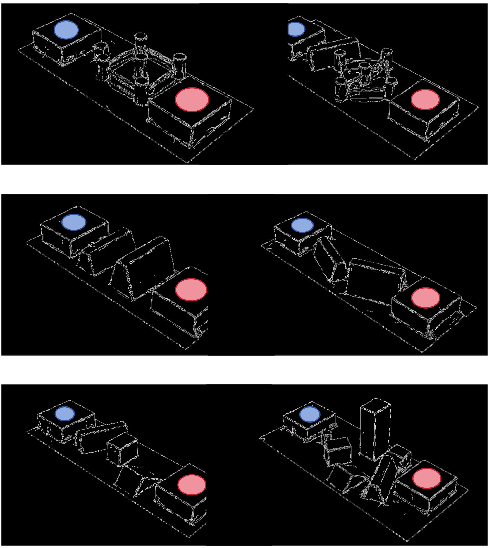
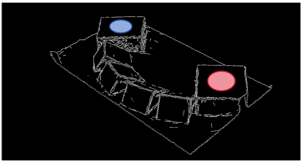
Figures 7–9 retain all thirteen course layouts and dimension annotations, including all six panels of the two-page Figure 7. Red marks the start and blue the goal. These exact layouts contextualize the narrow contact surfaces and prevent treating similarly named courses as interchangeable.
Appendix G Cross-Terrain Transfer
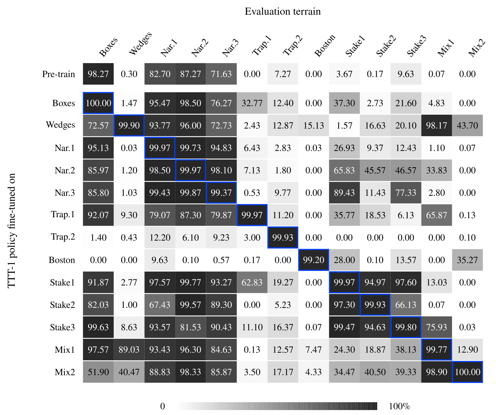
Figure 10 preserves the complete cross-terrain matrix: thirteen specialists plus the pretrained row, evaluated on all thirteen courses. Transfer is strongest among related beams/stakes. Stake1 transfers at 94.97% to Stake2 and 97.60% to Stake3, while Trapezoid2 is poor on most other courses.
Good diagonal performance does not establish broad retention. The original generalist is retained separately for other environments; a checkpoint-selection strategy is different from demonstrating that each adapted controller preserves all original skills.