Intuition. Instead of guessing every action and repeatedly simulating the whole journey, imagine placing tentative waypoints first and adjusting all neighboring transitions together. GRASP treats these intermediate latent states as optimization variables, adds a penalty when neighboring states disagree with the learned dynamics, and injects noise to escape poor routes. It also blocks unreliable gradients through state inputs while keeping useful action gradients, then periodically refines the plan with an ordinary rollout-based update. The method is primarily a planner for an existing differentiable world model, not a new JEPA representation-learning objective. Visual-control experiments report its strongest advantage at long horizons. Its theoretical analyses use restricted smooth or linear settings; practical stochastic, detached updates do not guarantee a globally feasible optimum.
1 Introduction
Long rollouts create long chains of derivatives and difficult local minima. Classical multiple shooting already introduces intermediate states; this paper adapts that idea to learned visual dynamics whose state derivatives may be brittle. GRASP combines lifted states, stochastic exploration, detached state-input gradients, and occasional full-rollout synchronization. Its gains depend on these components working together and on the quality of the underlying world model.
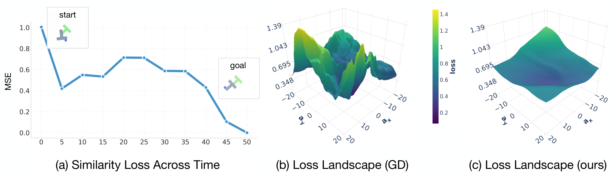
Figure 1: Difficulty of the planning problem. Subfigure (a) shows the distance to the goal in norm throughout a successful trajectory. This illustrates the difficulty of planning optimization away from a minimizer: successful trajectories often have to first move away from the goal to successfully plan towards it later, resulting in greedy strategies failing. Subfigures (b)-(c) depict the loss landscape at convergence of standard rollout-based planners vs. our planner. The example given is in the Push-T environment at horizon length 50. The axes plotted over are with respect to two random, orthogonal, unit-norm directions in the full action space . Our planner loss is taken as in Eq. (10), and for GD the loss is taken as in Eq. (3).
2 Problem formulation
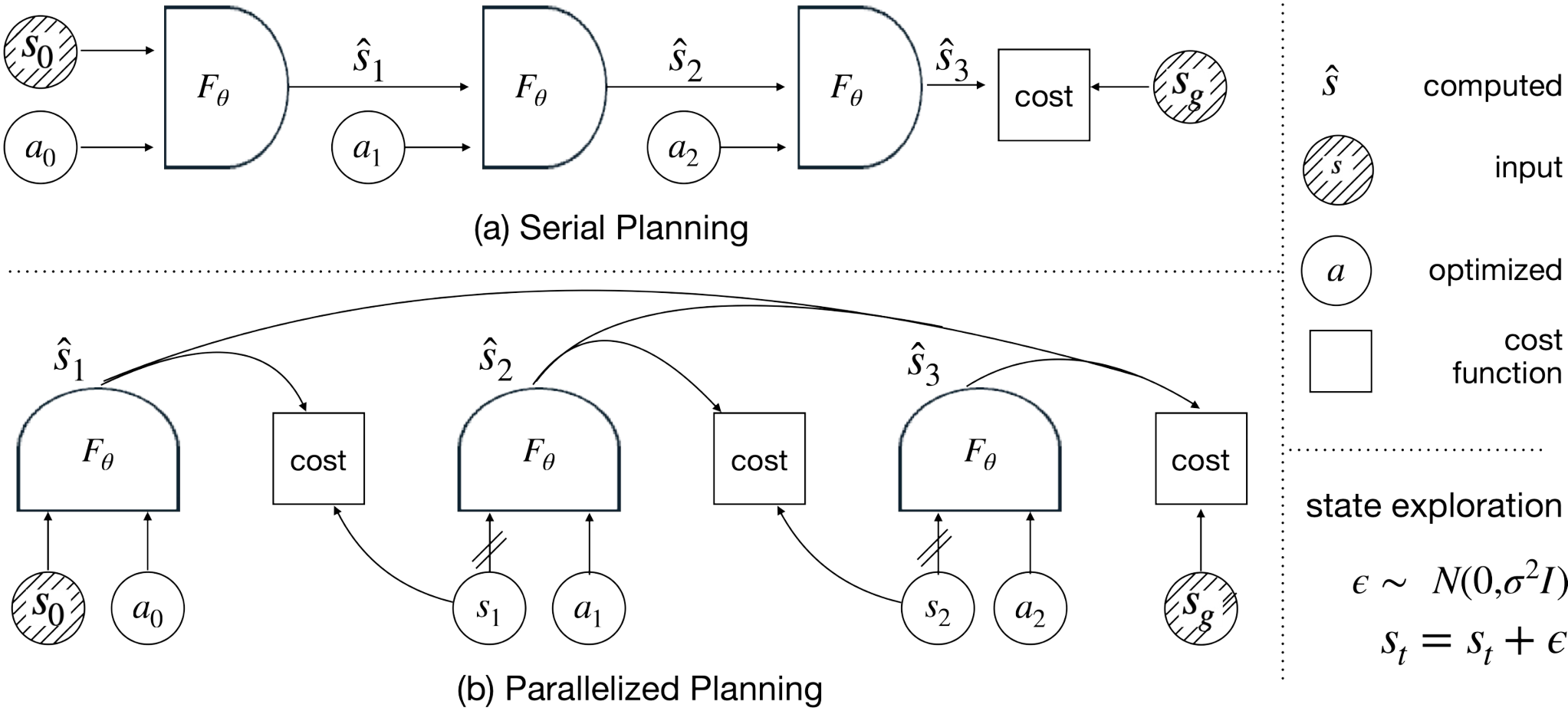
The task is to choose a continuous action sequence that makes a predicted final state approach a specified goal. Ordinary shooting generates every intermediate state serially from the first. This is computationally expensive and can produce poorly conditioned derivatives as the horizon grows. The paper instead introduces auxiliary state variables so that neighboring transitions can be evaluated in parallel.
Figure 2: Graphical depiction of (a) a standard serial-based setup for optimization-based planning, where states are rolled out using the actions and the loss is evaluated on the goal state, (b) our setup, which parallelizes the world model evaluations by optimizing “virtual states” directly and only supervising pairwise dynamics satisfaction. The crossed lines and skipped connections for our method’s depiction (b) are detailed in Section 3.3, which keeps the full planning graph connected while not requiring state gradients of the dynamics . For our planner, we find it helpful to alternate between (a) and (b) throughout the planning optimization.Equations 1–3
(1)
(2)
(3)
3 Decoupling dynamics for gradient-based planning
A soft dynamics penalty links free intermediate states to one-step predictions. This replaces a deeply composed rollout objective with many local consistency terms. The relaxation improves parallelism but temporarily permits imagined states that no action sequence can realize, so obtaining low relaxed loss and obtaining an executable plan must be distinguished.
3.1 Parallelized planning
All adjacent transition penalties can be evaluated simultaneously. Their global solutions correspond to the intended planning formulation under its stated conditions, but local optimization may still settle on implausible paths through obstacles. Learned high-dimensional dynamics also offer adversarial state directions. Subsequent components specifically address these two failures rather than assuming lifting solves them.
Equation 4
(4)
3.2 Exploration via Langevin state updates
Gaussian noise perturbs the optimized intermediate states to explore alternatives around poor local routes. This is exploration during planning optimization, not a stochastic environment model and not additional training data.
Langevin dynamics on state iterates.
Each state update combines a descent step and an independent Gaussian perturbation. The motivation is to escape narrow basins in the relaxed loss landscape. The later detached-gradient variant changes the vector field, so its complete practical update should not be identified with exact Langevin sampling.
Equations 5–6
(5)
(6)
Noise on states vs. actions.
Direct state perturbations can discover an intermediate waypoint without first finding the precise action sequence leading there. Dynamics penalties encourage those exploratory states to become locally consistent. This is different from injecting noise only into actions and propagating it through a long rollout.
(a)Expected behavior
(b)Adversarial example
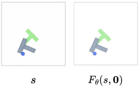
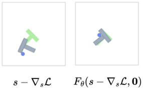
Figure 3: Sensitivity of state gradient structure. Examples of three states far away from the goal on the right (either in-distribution or out-of-distribution), such that taking a small step along the gradient , leads to a nearby state that solves the planning problem in a single step: . Thus, optimizing states directly through the world model can be quite challenging.
3.3 Sensitivity to state gradients
A note on adversarial robustness of state gradients.
The optimizer can exploit tiny off-manifold state changes that make a learned model predict a desired output, rather than finding a physically meaningful transition. The paper therefore removes derivatives through state inputs. Its impossibility result explains the resulting compromise: for a general dynamics family, exact dynamics-enforcing minimizers cannot simultaneously ignore all such state derivatives.
Equation 7
(7)
Figure 4: Virtual states learned through planning. All examples are instantiations of our planner at horizon 50 in the Point-Maze, Wall-Single, and Push-T environments. Regardless of the dynamics constraint relaxation and state noising, directly optimized states find realistic, non-greedy paths towards the goal.
Grad-cut dynamics loss.
A stop-gradient copy has the same numerical state value but contributes no derivative through the dynamics input. Gradients still update actions and the next-state consistency target. This deliberately changes the optimization rule; it is not ordinary gradient descent on the original planning objective.
Equation 8
(8)
Dense goal shaping on one-step predictions.
Without an additional goal signal, detached updates tend to stay near a current rollout. A goal penalty on every one-step prediction supplies action-directed progress at all time steps. Combined noisy updates favor locally consistent, goal-directed trajectories, but the states no longer follow a true gradient field or an exact Boltzmann sampler.
Equations 9–12
(9)
(10)
(11)
(12)
3.4 Full-rollout synchronization
Periodic synchronization addresses the gap between the relaxed stochastic search and an ordinary rollout. A brief refinement phase optimizes actions through the full model composition, using the original goal-reaching loss.
Full-gradient rollout step.
At a chosen cadence, a small number of full-backpropagation action updates refine the trajectory. The practical algorithm therefore mixes robust local search with occasional exposure to the brittle long-rollout derivatives it otherwise avoids. Both cadence and refinement count are consequential hyperparameters.
Equations 13–15
(13)
(14)
(15)
4 Results
The experiments ask whether lifting and noise escape greedy solutions, remain effective at long horizons, and improve time to a successful plan. The retained trajectories and ablations show why success alone is insufficient: an implausible relaxed path must eventually agree with executable dynamics.
Table 1: Open-loop planning results on long range Push-T. Reported are success rate (%) and median success time (seconds; successful trials only) across planning horizons. 500 trials per setting. Each cell reports Success / Time.
4.1 Baselines
Comparators are cross-entropy sampling, direct action-gradient descent, and a lifted LatCo-style optimizer. Hyperparameters are searched separately by task and horizon. GRASP initializes virtual states near an interpolated start–goal path and actions near zero; this initialization is part of the evaluated recipe.
(a)Point Maze ()
(b)Push-T ()
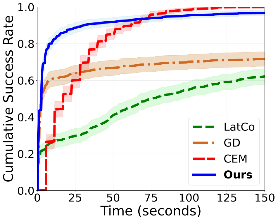
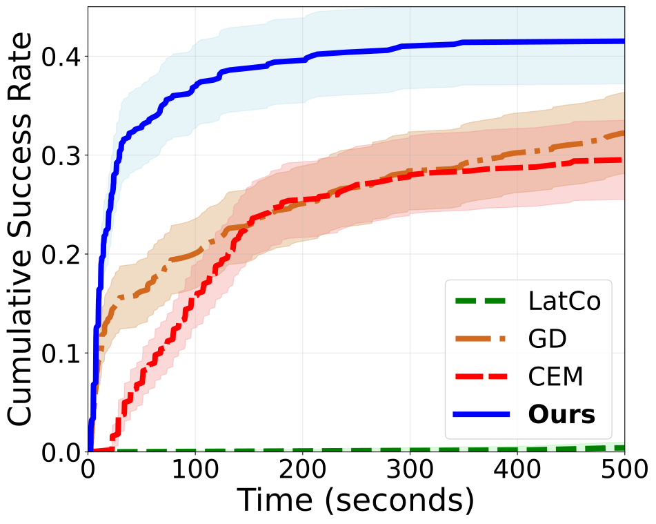
Figure 5: Success rate over time at a fixed horizon. Success rate over fixed set of open-loop planning tasks for CEM, GD, LatCo (Rybkin et al., 2021), and our planner for a fixed horizon of 50. Curves summarize how quickly each planner makes progress under the learned world model setting when evaluated at a fixed planning horizon. Shaded regions are Wald 95% confidence intervals.
4.2 Environments and evaluation protocol
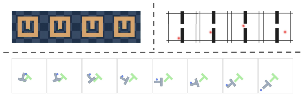
PointMaze, Wall-Single, and Push-T use visual world models trained through the DINO-WM framework. A model step consumes action chunks and predicts several physical steps. The reported protocol defines goal-reaching over these learned-model planning tasks; it should not be generalized into a claim of real-robot deployment.
4.3 Long-term planning and horizon scaling
The main gains occur when longer horizons require non-greedy routes. GRASP solves more evaluated tasks and reaches successful plans faster than the selected baselines in those regimes. The success-versus-time plots complement median times, since a median over successful trials alone hides failures.
Table 2: Ablation Studies over the GD sync steps, level of noise for Langevin dynamics, and whether we use our detached gradient approach with the goal-reaching objective or not. GD sync happens every 100 stochastic steps. Ablations done on the Push-T environment at horizon . Time reported is median over successful trials, which only beats our method when the accuracy is much smaller.
Table 3: Short Term Planning. Success rate (%) for Push-T, PointMaze, and WallSingle. 500 trials per setting. Our method has comparable success rate while having a consistently low completion time (Table 4).
Table 4: Median completion times (seconds) across short-term experiments. 500 trials per setting. Our method has a consistently low completion time with a comparable success rate (Table 3).
4.4 Short-term planning
At shorter horizons, the method is generally competitive rather than uniformly superior. Its extra exploration can cost time relative to a simpler gradient planner while improving success. The full success and timing tables should be read together rather than reducing the result to one universal speedup.
5 Related work
The method connects sampling planners, differentiable trajectory optimization, multiple shooting, and noisy optimization. Its distinctive contribution is the combination suited to imperfect learned visual dynamics. It does not claim to introduce state lifting itself, and unlike world-model adversarial training it leaves the existing predictor unchanged.
6 Limitations and future work
Benefits shrink on short easy tasks, and several stabilizing components require tuning. A smoother learned state geometry could reduce the need for detached gradients and synchronization. Hybridizing GRASP with other planners is left open. No empirical result establishes global optimality or removes errors in the learned dynamics.
7 Conclusion
The paper demonstrates that planner design can substantially change the usefulness of the same learned world model. Time-parallel virtual states and action-focused gradient updates are especially useful in its long-horizon experiments; successful application still depends on representation geometry, model fidelity, and optimization settings.
Appendix A Theory
The appendix separates several restricted analytical arguments: conditioning of lifted objectives, Gaussian smoothing, the distribution induced by state-only noise, and the consequences of stop-gradient updates. These motivate individual components but do not combine into a global convergence proof for the full nonlinear planner.
A.1 Convergence of various methods in the convex setting
A linear-system analysis compares the horizon dependence of shooting and lifted optimization. The useful distinction is the smoothness of the optimization landscape, not a guarantee that every learned visual dynamics model satisfies the convex assumptions.
Equations 16–20
(16)
(17)
(18)
(19)
subject to
(20)
Shooting Method.
Composing an unstable linear dynamics model can make the shooting Hessian grow exponentially with horizon under the stated reachability assumptions. This explains why a step size safe for a short rollout can fail on a much longer one.
Equations 21–22
(21)
(22)
Lifted Method.
The lifted objective produces a sparse, locally coupled quadratic system. Its Hessian norm is bounded using the one-step state and action matrices rather than their long products. The resulting upper bound is independent of horizon, although conditioning and feasibility still require their own assumptions.
Equations 23–38
(23)
(24)
(25)
(26)
(27)
(28)
(29)
(30)
(31)
(32)
(33)
(34)
(35)
(36)
(37)
(38)
Interpretation.
Lifting acts as a form of optimization preconditioning by replacing long dependencies with neighboring constraints. The horizon-independent smoothness result belongs to the analyzed linear objective; it is motivation for, not a blanket guarantee about, the nonlinear experiments.
A.2 Gaussian noise regularization
Gaussian convolution smooths a loss, with gradient bounds controlled by noise variance under integrability assumptions. Noisy updates consequently see smoothed gradients in expectation. Annealing noise trades broad exploration for more precise local refinement; the theorem does not choose an optimal finite noise schedule.
Equations 39–55
(39)
(40)
(41)
(42)
(43)
(44)
(45)
(46)
(47)
(48)
(49)
(50)
(51)
(52)
(53)
(54)
(55)
A.3 Connection to Boltzmann sampling, state-only noising
Adding properly matched noise to all variables can yield a Gibbs stationary distribution under suitable conditions. GRASP perturbs states but not actions, so that standard Boltzmann interpretation does not apply directly. The appendix describes its more constrained action-conditioned behavior rather than claiming exact equilibrium sampling.
Equations 56–57
(56)
(57)
A.4 State-gradient-free Dynamics
The appendix proves that a general exact dynamics-enforcing objective cannot have state gradients independent of the dynamics Jacobian. For a linear detached update with positive goal weights and full-column-rank action matrix, it establishes convergence to a unique fixed point. That fixed point need not be a globally optimal feasible trajectory for the original nonlinear problem.
Equations 58–91
(58)
(59)
(60)
(61)
(62)
(63)
(64)
(65)
(66)
(67)
(68)
(69)
(70)
(71)
(72)
(73)
(74)
(75)
(76)
(77)
(78)
(79)
(80)
(81)
(82)
(83)
(84)
(85)
(86)
(87)
(88)
(89)
(90)
(91)
Notes on the stopgrad optimization.
With one-step predictions held fixed, noisy virtual-state updates form a Gaussian neighborhood around those predictions. Action updates move that neighborhood toward the goal through controllable directions. Ordinary noisy rollouts instead propagate randomness through time and can drift or spread. These conditional calculations clarify the mechanism while retaining their fixed-center, linearization, and stability assumptions.
Equations 92–105
(92)
(93)
(94)
(95)
(96)
(97)
(98)
(99)
(100)
(101)
(102)
(103)
(104)
(105)
Appendix B Ablations
The Push-T ablations isolate noise, detached state gradients, and synchronization, and also compare simpler action- or rollout-noise variants. Their combination is strongest in the tested setup. Noise cannot be treated as interchangeable across state optimization and action rollout, and the ablation does not establish one setting for every horizon.
Equations 106–107
(106)
(107)
Appendix C Additional experiments
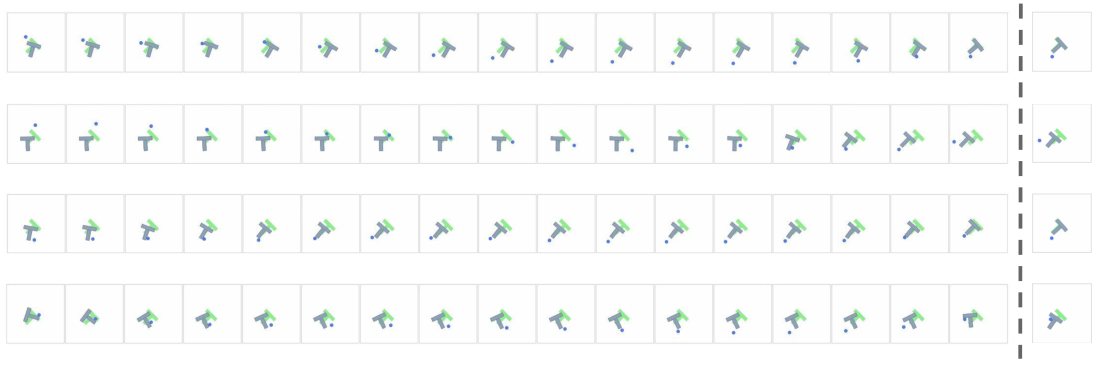
The additional visual examples expose both successful relaxed trajectories and a bad local minimum that crosses an obstacle. They are useful checks of what the optimizer is doing internally; selected examples supplement the quantitative evaluation rather than replacing it.
Table 5: Stochastic GD Baselines Ablation Study, showing alternatives from our method for a stochastic gradient-based planner. For rollouts of the world model , values of correspond to variance of noise added to actions throughout optimization, and values of correspond to noise added to states directly through the rollout; that is, for rollouts of the world model, . None beat our method’s performance, shown in Table 2. Reported time is average time over all experiments, with reported intervals as 95% CI.
Setting
Accuracy (%)
Time (s)
Default Mode (objective.mode=default)
53.0 4.4
864 77
50.6 4.4
913.97 78
37.2 4.3
1149 75
47.6 4.4
1056 73
53.0 4.4
864 77
33.4 4.2
1208 73
53.8 4.4
854 78
Mode All (objective.mode=all)
54.0 4.4
865 77
55.8 4.4
838 77
41.0 4.4
1111 75
46.6 4.4
1067 73
52.8 4.4
873 77
52.4 4.4
878 77
55.8 4.4
838 77
Figure 6: Example of converged plans for our planner on the Push-T environment at horizon 80, with goals depicted to the right of the dashed line. The parallel optimization is able to converge more consistently at longer horizons, and find the required non-greedy paths to the goal.Figure 7: Example of a bad local minima when relaxing the dynamics constraint into a penalty function. The dynamics are nonzero for the middle transition, but both the states and actions are at a local minima; there’s no direction they can move locally to reduce the dynamics loss further.
42 references
Ascher et al. (1995)U. M. Ascher, R. M. Mattheij, and R. D. RussellNumerical solution of boundary value problems for ordinary differential equations.
SIAM.
Assran et al. (2025)M. Assran, A. Bardes, D. Fan, Q. Garrido, R. Howes, M. Muckley, A. Rizvi, C. Roberts, K. Sinha, A. Zholus, et al.V-jepa 2: self-supervised video models enable understanding, prediction and planning.
arXiv preprint arXiv:2506.09985.
Ball et al. (2025)P. J. Ball, J. Bauer, F. Belletti, B. Brownfield, A. Ephrat, S. Fruchter, A. Gupta, K. Holsheimer, A. Holynski, J. Hron, C. Kaplanis, M. Limont, M. McGill, Y. Oliveira, J. Parker-Holder, F. Perbet, G. Scully, J. Shar, S. Spencer, O. Tov, R. Villegas, E. Wang, J. Yung, C. Baetu, J. Berbel, D. Bridson, J. Bruce, G. Buttimore, S. Chakera, B. Chandra, P. Collins, A. Cullum, B. Damoc, V. Dasagi, M. Gazeau, C. Gbadamosi, W. Han, E. Hirst, A. Kachra, L. Kerley, K. Kjems, E. Knoepfel, V. Koriakin, J. Lo, C. Lu, Z. Mehring, A. Moufarek, H. Nandwani, V. Oliveira, F. Pardo, J. Park, A. Pierson, B. Poole, H. Ran, T. Salimans, M. Sanchez, I. Saprykin, A. Shen, S. Sidhwani, D. Smith, J. Stanton, H. Tomlinson, D. Vijaykumar, L. Wang, P. Wingfield, N. Wong, K. Xu, C. Yew, N. Young, V. Zubov, D. Eck, D. Erhan, K. Kavukcuoglu, D. Hassabis, Z. Gharamani, R. Hadsell, A. van den Oord, I. Mosseri, A. Bolton, S. Singh, and T. RocktäschelGenie 3: a new frontier for world models.
External Links:
Bar et al. (2025)A. Bar, G. Zhou, D. Tran, T. Darrell, and Y. LeCunNavigation world models.
In Proceedings of the Computer Vision and Pattern Recognition Conference,
pp. 15791–15801.
Bharadhwaj et al. (2020)H. Bharadhwaj, K. Xie, and F. ShkurtiModel-predictive control via cross-entropy and gradient-based optimization.
In Learning for Dynamics and Control,
pp. 277–286.
Bock and Plitt (1984)H. G. Bock and K. PlittA multiple shooting algorithm for direct solution of optimal control problems.
IFAC Proceedings Volumes17 (2), pp. 1603–1608.
Bordalba et al. (2022)R. Bordalba, T. Schoels, L. Ros, J. M. Porta, and M. DiehlDirect collocation methods for trajectory optimization in constrained robotic systems.
IEEE Transactions on Robotics39 (1), pp. 183–202.
Bras (2023)P. BrasLangevin algorithms for very deep neural networks with application to image classification.
Procedia Computer Science222, pp. 303–310.
Chaudhari et al. (2019)P. Chaudhari, A. Choromanska, S. Soatto, Y. LeCun, C. Baldassi, C. Borgs, J. Chayes, L. Sagun, and R. ZecchinaEntropy-sgd: biasing gradient descent into wide valleys.
Journal of Statistical Mechanics: Theory and Experiment2019 (12), pp. 124018.
Diedam and Sager (2018)H. Diedam and S. SagerGlobal optimal control with the direct multiple shooting method.
Optimal Control Applications and Methods39 (2), pp. 449–470.
Ding et al. (2024)J. Ding, Y. Zhang, Y. Shang, Y. Zhang, Z. Zong, J. Feng, Y. Yuan, H. Su, N. Li, N. Sukiennik, et al.Understanding world or predicting future? a comprehensive survey of world models.
ACM Computing Surveys.
Foret et al. (2020)P. Foret, A. Kleiner, H. Mobahi, and B. NeyshaburSharpness-aware minimization for efficiently improving generalization.
arXiv preprint arXiv:2010.01412.
Fu et al. (2020)J. Fu, A. Kumar, O. Nachum, G. Tucker, and S. LevineD4rl: datasets for deep data-driven reinforcement learning.
arXiv preprint arXiv:2004.07219.
Gelfand and Mitter (1991)S. B. Gelfand and S. K. MitterRecursive stochastic algorithms for global optimization in rˆd.
SIAM Journal on Control and Optimization29 (5), pp. 999–1018.
Goswami et al. (2025)R. G. Goswami, A. Bar, D. Fan, T. Yang, G. Zhou, P. Krishnamurthy, M. Rabbat, F. Khorrami, and Y. LeCunWorld models can leverage human videos for dexterous manipulation.
arXiv preprint arXiv:2512.13644.
Guhathakurta et al. (2022)D. Guhathakurta, F. Rastgar, M. A. Sharma, K. M. Krishna, and A. K. SinghFast joint multi-robot trajectory optimization by gpu accelerated batch solution of distributed sub-problems.
Frontiers in Robotics and AI9, pp. 890385.
Guo et al. (2025)Y. Guo, L. X. Shi, J. Chen, and C. FinnCtrl-world: a controllable generative world model for robot manipulation.
arXiv preprint arXiv:2510.10125.
Huang et al. (2021)K. Huang, S. Lale, U. Rosolia, Y. Shi, and A. AnandkumarCem-gd: cross-entropy method with gradient descent planner for model-based reinforcement learning.
arXiv preprint arXiv:2112.07746.
Jerez et al. (2011)J. L. Jerez, E. C. Kerrigan, and G. A. ConstantinidesA condensed and sparse qp formulation for predictive control.
In 2011 50th IEEE Conference on Decision and Control and European Control Conference,
pp. 5217–5222.
Koju et al. (2025)S. Koju, S. Bastola, P. Shrestha, S. Amgain, Y. R. Shrestha, R. P. Poudel, and B. BhattaraiSurgical vision world model.
In MICCAI Workshop on Data Engineering in Medical Imaging,
pp. 1–10.
Lai et al. (2022)T. Lai, W. Zhi, T. Hermans, and F. RamosParallelised diffeomorphic sampling-based motion planning.
In Conference on robot learning,
pp. 81–90.
Nie and Kerrigan (2025)Y. Nie and E. C. KerriganReliable solution to dynamic optimization problems using integrated residual regularized direct collocation.
arXiv preprint arXiv:2503.09123.
Parthasarathy et al. (2025)A. Parthasarathy, N. Kalra, R. Agrawal, Y. LeCun, O. Bounou, P. Izmailov, and M. GoldblumClosing the train-test gap in world models for gradient-based planning.
arXiv preprint arXiv:2512.09929.
Pinneri et al. (2021)C. Pinneri, S. Sawant, S. Blaes, J. Achterhold, J. Stueckler, M. Rolinek, and G. MartiusSample-efficient cross-entropy method for real-time planning.
In Conference on Robot Learning,
pp. 1049–1065.
Piovesan and Tanner (2009)J. L. Piovesan and H. G. TannerRandomized model predictive control for robot navigation.
In 2009 IEEE International Conference on Robotics and Automation,
pp. 94–99.
Rubinstein and Kroese (2004)R. Y. Rubinstein and D. P. KroeseThe cross-entropy method: a unified approach to combinatorial optimization, monte-carlo simulation and machine learning.
Springer Science & Business Media.
Rybkin et al. (2021)O. Rybkin, C. Zhu, A. Nagabandi, K. Daniilidis, I. Mordatch, and S. LevineModel-based reinforcement learning via latent-space collocation.
In International Conference on Machine Learning,
pp. 9190–9201.
Shamir et al. (2021)A. Shamir, O. Melamed, and O. BenShmuelThe dimpled manifold model of adversarial examples in machine learning.
arXiv preprint arXiv:2106.10151.
Szegedy et al. (2013)C. Szegedy, W. Zaremba, I. Sutskever, J. Bruna, D. Erhan, I. Goodfellow, and R. FergusIntriguing properties of neural networks.
arXiv preprint arXiv:1312.6199.
Tamimi and Li (2009)J. Tamimi and P. LiNonlinear model predictive control using multiple shooting combined with collocation on finite elements.
IFAC Proceedings Volumes42 (11), pp. 703–708.
Tassa et al. (2018)Y. Tassa, Y. Doron, A. Muldal, T. Erez, Y. Li, D. d. L. Casas, D. Budden, A. Abdolmaleki, J. Merel, A. Lefrancq, et al.Deepmind control suite.
arXiv preprint arXiv:1801.00690.
Von Stryk (1993)O. Von StrykNumerical solution of optimal control problems by direct collocation.
In Optimal Control: Calculus of Variations, Optimal Control Theory and Numerical Methods,
pp. 129–143.
Welling and Teh (2011)M. Welling and Y. W. TehBayesian learning via stochastic gradient langevin dynamics.
In Proceedings of the 28th international conference on machine learning (ICML-11),
pp. 681–688.
Williams et al. (2016)G. Williams, P. Drews, B. Goldfain, J. M. Rehg, and E. A. TheodorouAggressive driving with model predictive path integral control.
In 2016 IEEE international conference on robotics and automation (ICRA),
pp. 1433–1440.
Xu et al. (2018)P. Xu, J. Chen, D. Zou, and Q. GuGlobal convergence of langevin dynamics based algorithms for nonconvex optimization.
Advances in Neural Information Processing Systems31.
Zhou et al. (2024)G. Zhou, H. Pan, Y. LeCun, and L. PintoDino-wm: world models on pre-trained visual features enable zero-shot planning.
arXiv preprint arXiv:2411.04983.