Overview
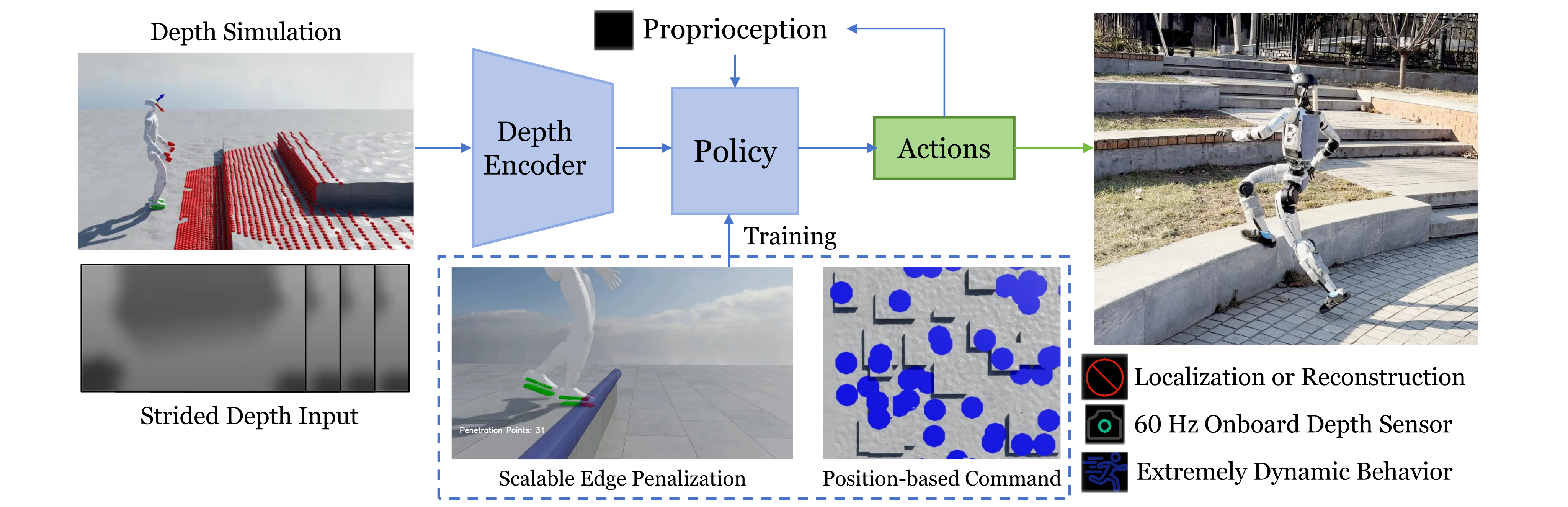
This framework learns humanoid locomotion directly from depth history and proprioception. Its distinctive training mechanisms penalize unsafe edge contacts and generate velocity commands toward flat terrain patches.
At a glance
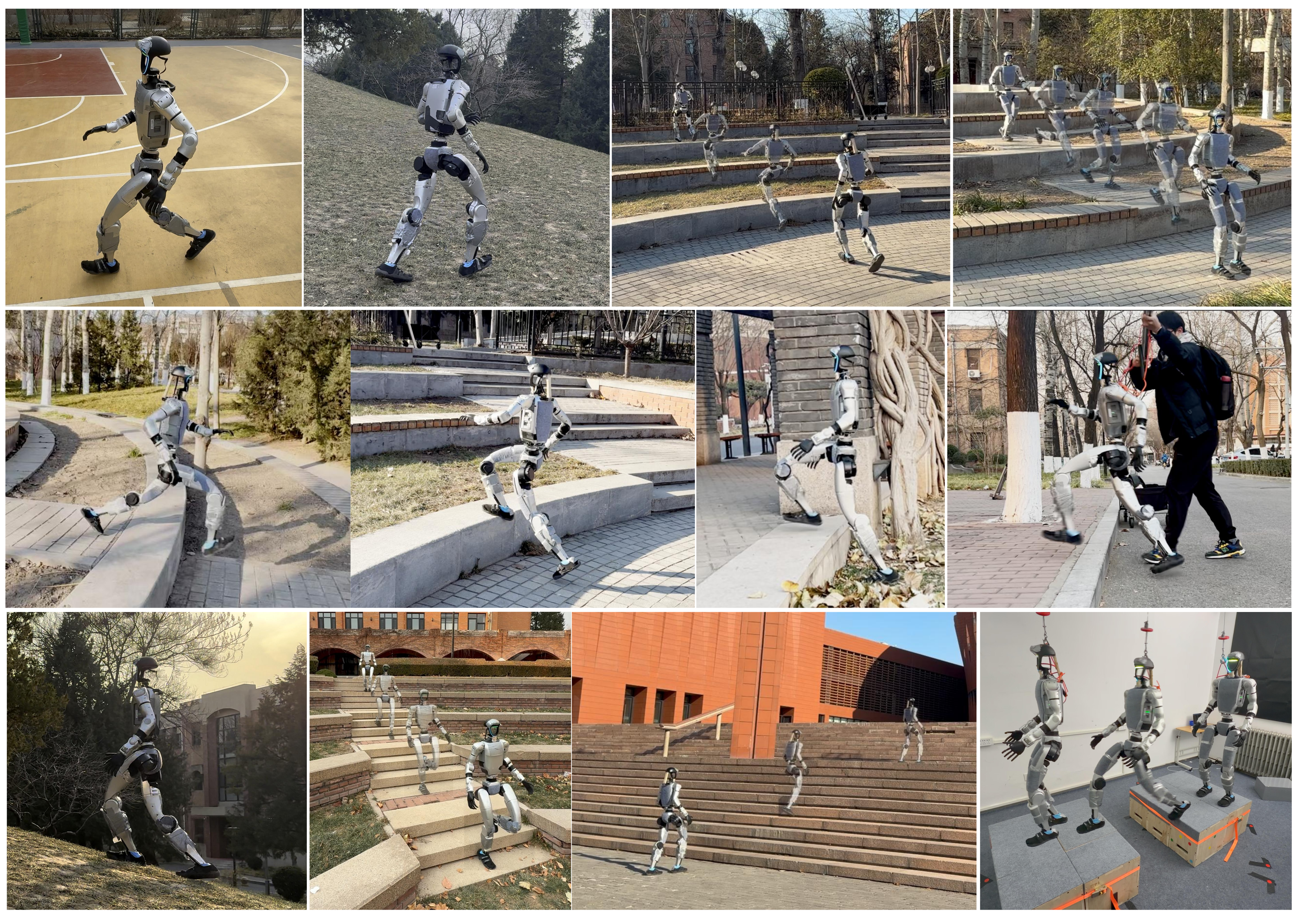
Depth-based policies transfer from simulation to a Unitree G1 and demonstrate walking, running and obstacle traversal. Mesh edge detection plus foot volume points encourage centered footholds; flat-patch goals reduce unproductive turning during training. Hardware reaches a reported peak 2.5 m/s, with separate deployment policies and human velocity guidance. The study does not demonstrate one autonomous policy handling every terrain.
1 Introduction
The task is legged obstacle traversal using foot contacts, excluding arm-assisted climbing, vaulting and other whole-body contact maneuvers. Depth observations provide advance terrain information that blind locomotion lacks, without maintaining an external localization system or explicit elevation map.
This edition covers all 22 pages of arXiv v2, dated 13 October 2026, with the exact title and all five authors verified; the catalog retains its January preprint date. End-to-end refers to depth/proprioception-to-joint control. Training still uses simulator geometry, motion priors and structured rewards; deployment remains operator-guided.
2 Related Work
The paper situates direct depth control alongside learned legged locomotion and explicit foothold planning.
2.1 Learning-based Legged Locomotion
Blind RL handles many disturbances but cannot anticipate large gaps. Perceptive alternatives reconstruct elevation/voxel maps or learn directly from images. This approach uses recent depth at high acquisition frequency; its comparison with a 10 Hz height map changes both representation and practical operating rate, so it does not isolate representation alone.
2.2 Perceptive Foothold Control
Explicit foothold planners choose placements from geometric maps and feasibility costs. Implicit policies instead learn contact preferences through penalties. The proposed detector extends the latter approach to triangle meshes, avoiding terrain-specific edge annotations while retaining threshold and geometric-model assumptions.
3 Method
Train a depth-conditioned controller, regularize foot contacts using mesh geometry, and expose it to meaningful traversal commands. These training-only geometric mechanisms are not an online map reconstruction module.
3.1 Problem Formulation
Train an asymmetric actor–critic with PPO. The actor receives noisy angular velocity, projected gravity, velocity commands, joints, previous actions and depth history; the critic additionally receives clean states and base linear velocity. The actor outputs 29 target joint positions tracked by PD control.
The simulator generates training commands automatically. On hardware, a person supplies velocity commands through a remote controller. Termination and reward rules penalize falls and unsafe configurations rather than guaranteeing safety.
3.2 Ego-centric Depth Perception
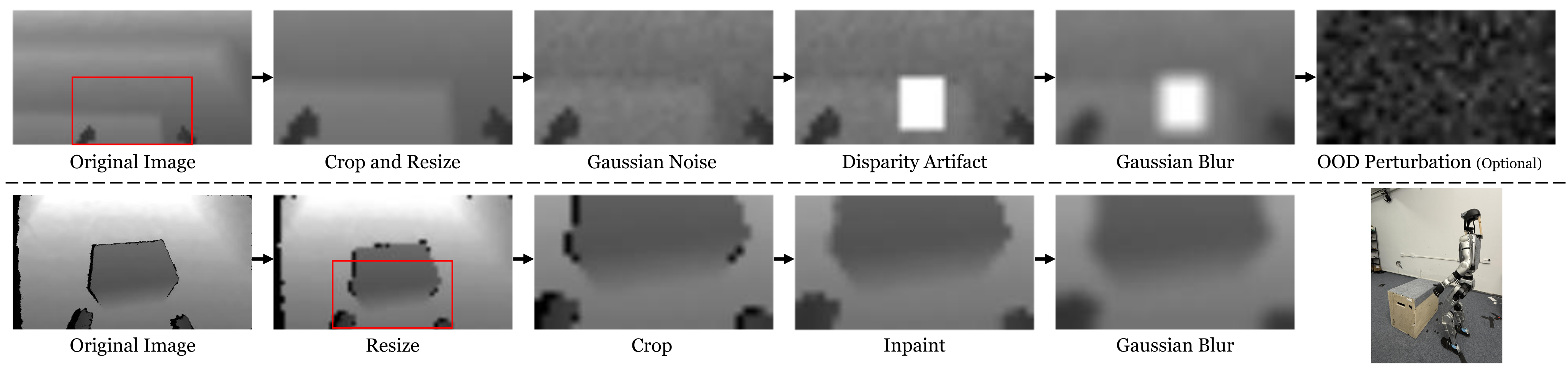
A NVIDIA Warp ray-caster synthesizes depth. Simulation adds range noise, disparity failures, blur and occasional complete corruption; hardware inpaints invalid pixels and blurs the stream. Both paths aim to make input distributions similar.
Depth acquisition/preprocessing runs asynchronously at 60 Hz; policy inference runs at 50 Hz using the latest data. Eight strided depth frames provide temporal context, and training includes one-frame delay. These are distinct acquisition, control and history-sampling frequencies.
3.3 Terrain Edge Contact Penalization
Simulation can reward short, efficient steps that partly land on edges, even though these contacts may slip on hardware. A soft geometric penalty shifts the learned policy toward better-supported footholds.
3.3.1 Terrain Edge Detector
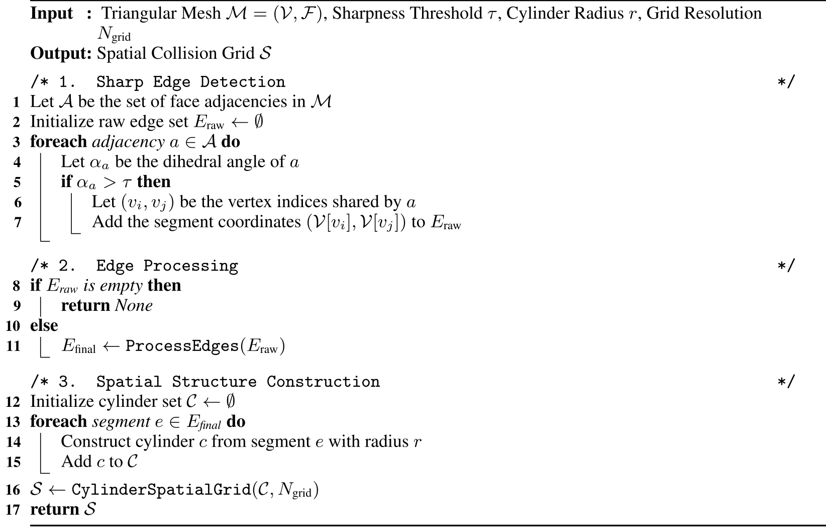
Compare adjacent triangle-face normals through their dihedral angle and retain edges above a sharpness threshold. Greedy collinear-segment merging reduces primitives before building a spatial collision structure. The method accepts arbitrary meshes; examples on new meshes demonstrate detection behavior, not a proof of reliable locomotion on every topology.

3.3.2 Volumetric Point Penetration Penalization
Sample points inside each foot’s collision shape. Query their penetration offsets relative to cylinders around detected edges, then sum penetration magnitude times point speed plus 10⁻³ (Equation 1). Table 5 gives this nonnegative quantity a negative reward weight of −4. Faster impacts/scraping are more costly, while the small constant still penalizes stationary penetration.
Equation 1
| (1) |
3.4 Position-based Velocity Command Generation
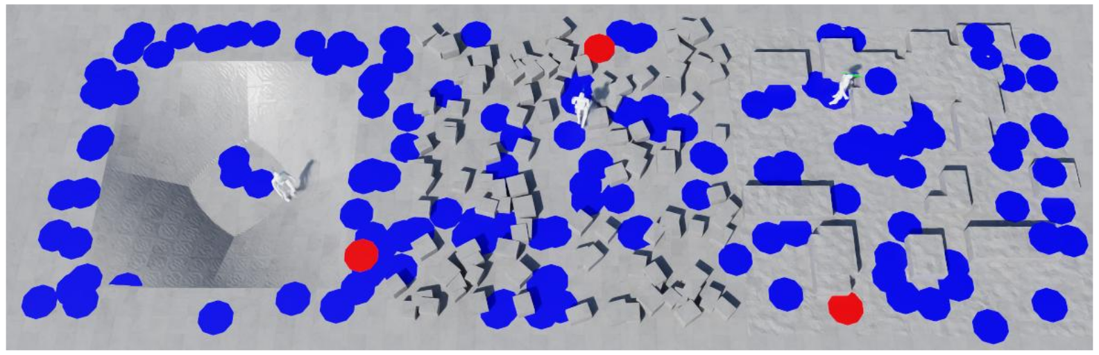
During training, select locally flat target patches and derive forward speed from target x-distance and yaw rate from its bearing, clipped to terrain-dependent limits. Lateral velocity is zero because the camera faces forward. Some flat-ground agents receive pure-turn commands to retain turning skill.
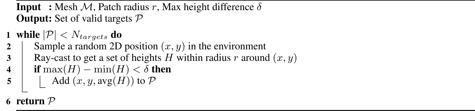
Flat-patch rejection sampling reduces obviously poor targets, but Algorithm 1 checks local height variation only. It does not itself prove that a collision-free, dynamically feasible route connects the robot to every accepted patch. The main text’s reachability language should be read with that limitation.
Equations 2–3
| (2) | ||||
| (3) |
3.5 Policy Training with Adversarial Motion Priors
Adversarial Motion Priors add style rewards from short motion sequences. Walking uses synthetic and retargeted human references; running uses a separate short gait cycle. Joint training produced long-stride fast walking, so the authors train walking and running separately rather than demonstrating seamless learned gait transitions.
4 Experiments
Simulation compares a single generalist walking policy per method. Running is excluded because it does not cover every benchmark terrain, including stairs. Hardware uses additional specialized policies, so simulation and deployment policy scope differ.
4.1 Real-world Deployment
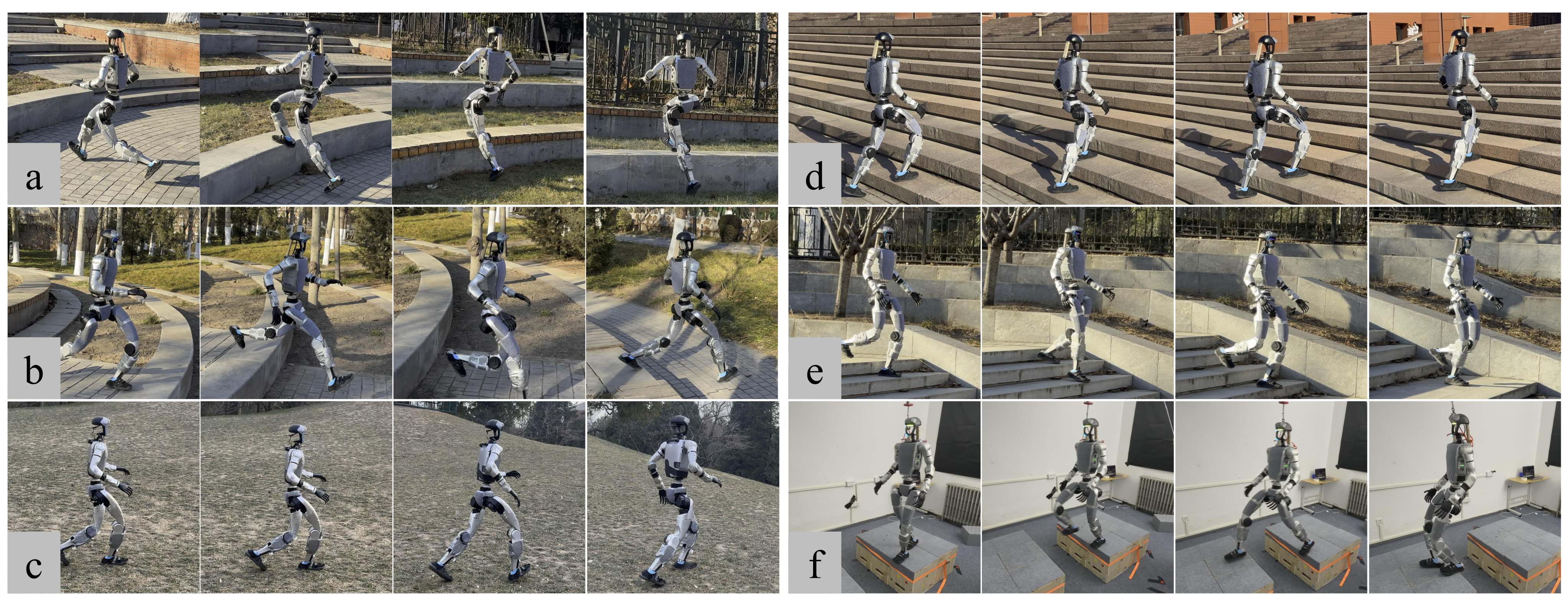
Hardware uses specialized stair-walking, platform-walking and running policies, with the general walking policy for other walking tasks. Switching requires stop, transition to a standing controller, then select the next policy. These policies receive extra simulator training; zero-shot describes transfer to hardware without real-world policy adaptation.
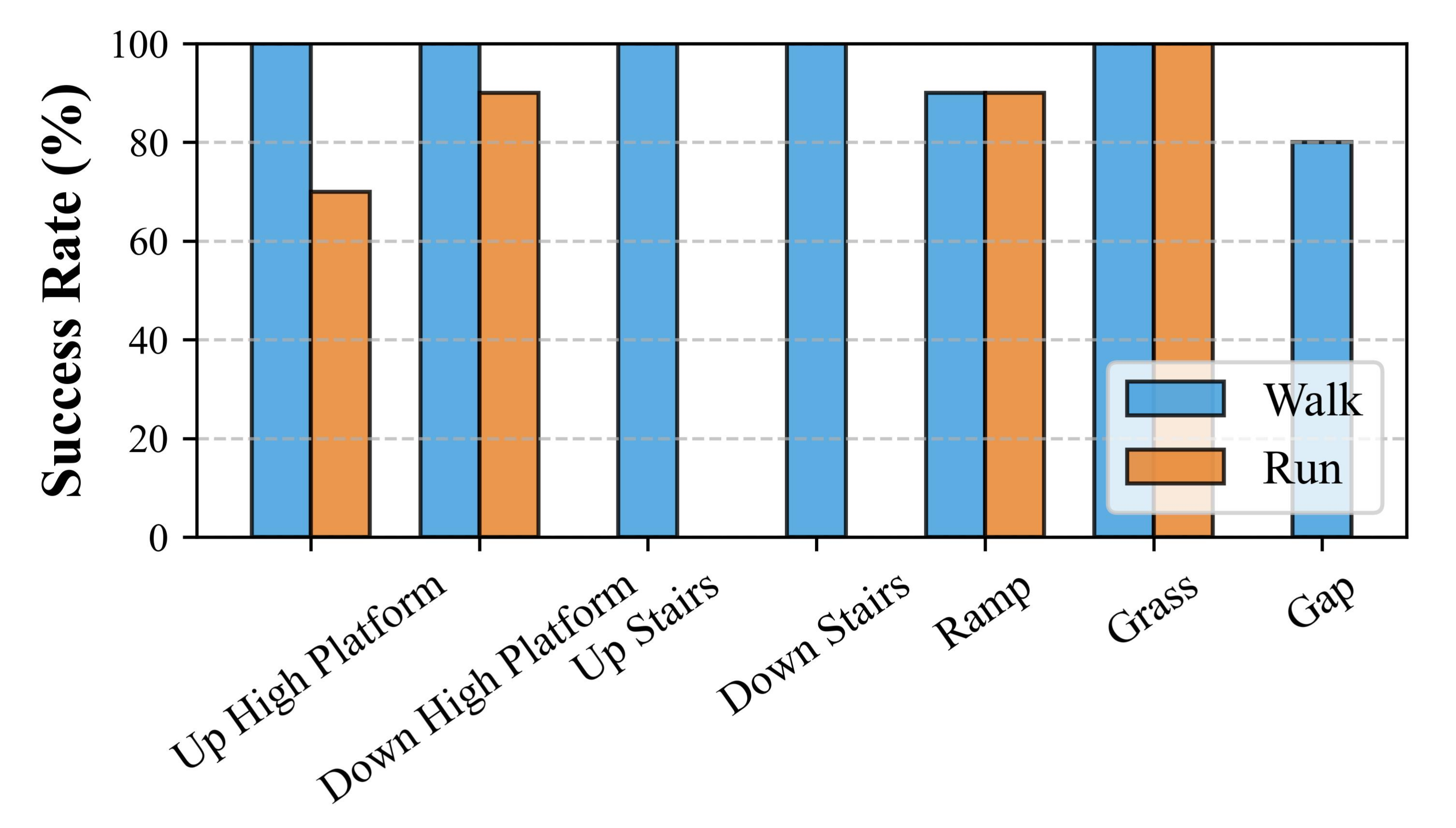
Reported limits include 2.5 m/s running, 32 cm platforms and 50 cm gaps, without claiming every gait reaches every limit. Figure 6 gives ten trials per evaluated terrain–gait pair: walking succeeds 10/10 on both platform directions, both stair directions and grass, 9/10 on ramp, and 8/10 on gap. Running gives 7/10 platform ascent, 9/10 descent, 9/10 ramp and 10/10 grass; missing running bars are untested combinations, not zero success.
A trial must reach its endpoint and stop stably; falling is failure. One four-minute stair/flat-ground run has no fall or physical assistance. This is useful endurance evidence but not a statistical guarantee of long-duration reliability or absence of operator guidance.
4.2 Edge-aware Penalization Mechanism
Measure landing-area fraction only while the base is in an obstacle’s interaction region, avoiding dilution by easy flat-ground contacts. Simulation uses 1,000 robots for 10,000 timesteps. Edge penalties raise supported foot area on stair up/down from 0.68/0.50 to 0.77/0.67, on deep gaps from 0.21 to 0.84, and on small boxes from 0.70 to 0.81.
Simulation success is similar or better, while hardware stair-up/down and gap counts improve from 8/10, 6/10 and 3/10 to 10/10, 10/10 and 8/10. These small trial sets support the claimed trend with limited precision. Stones, stakes and noisy scans illustrate detector extensibility; they are not additional quantified hardware terrain benchmarks.
| Sim SR | Landing Area | Real SR | ||||
|---|---|---|---|---|---|---|
| Terrain Type | Ours | No Edge | Ours | No Edge | Ours | No Edge |
| Stair Up | 100.00% | 100.00% | 0.77 | 0.68 | 10/10 | 8/10 |
| Stair Down | 99.95% | 99.82% | 0.67 | 0.50 | 10/10 | 6/10 |
| Deep Gap | 100.0% | 99.94% | 0.84 | 0.21 | 8/10 | 3/10 |
| Small Box | 99.09% | 93.17% | 0.81 | 0.70 | – | – |



Original selectable source
| Success Rate (%) | Mean Reaching Time (s) | ||||||||||||||||||
|---|---|---|---|---|---|---|---|---|---|---|---|---|---|---|---|---|---|---|---|
| Method | Large Box | Ramp | Small Box | Rough | Stair Down | Platform down | Stair Up | Platform up | Gap | Large Box | Ramp | Small Box | Rough | Stair Down | Platform down | Stair Up | Platform up | Gap | |
| w/o depth history | 100.0 | 100.0 | 1.66 | 100.0 | 99.88 | 100.0 | 100.0 | 100.0 | 100.0 | 6.20 | 6.72 | 11.68 | 5.78 | 5.33 | 5.81 | 6.54 | 5.89 | 5.79 | |
| w/o position-based | 23.13 | 100.0 | 90.68 | 100.0 | 99.59 | 100.0 | 95.18 | 11.70 | 100.0 | 9.41 | 5.74 | 11.32 | 5.72 | 6.77 | 7.07 | 6.79 | 10.57 | 5.70 | |
| w/o AMP | 13.75 | 99.94 | 0.00 | 100.0 | 98.39 | 99.47 | 0.00 | 0.00 | 99.94 | 9.81 | 5.68 | – | 6.50 | 6.89 | 7.40 | – | – | 6.07 | |
| 10Hz height map | 99.40 | 100.0 | 15.28 | 100.0 | 99.60 | 100.0 | 100.0 | 95.21 | 100.0 | 6.51 | 6.01 | 14.73 | 6.34 | 4.40 | 5.63 | 5.63 | 6.03 | 6.40 | |
| w/o depth | 38.94 | 100.0 | 3.33 | 100.0 | 99.12 | 99.93 | 94.54 | 0.00 | 67.95 | 7.88 | 8.48 | 10.59 | 7.75 | 5.39 | 6.72 | 7.12 | – | 7.58 | |
| HPL [54] | 43.65 | 99.71 | 51.01 | 100.0 | 99.90 | 100.0 | 92.07 | 97.84 | 99.95 | 8.30 | 6.16 | 9.65 | 8.22 | 6.10 | 6.13 | 6.34 | 5.99 | 7.44 | |
| Ours | 100.0 | 100.0 | 99.09 | 100.0 | 99.95 | 100.0 | 100.0 | 100.0 | 100.0 | 5.91 | 5.84 | 8.03 | 5.40 | 5.15 | 5.63 | 5.36 | 5.60 | 5.43 | |
4.3 Comparison and Ablation
Table 2 retains all success rates and successful-trial reaching times for depth-history, command-generation, AMP, blind, 10 Hz height-map and HPL comparisons. The full walking policy reaches 99.09% on small boxes, 99.95% stair down and 100% on the other listed terrains.
Removing depth history reduces small-box success to 1.66%; the height-map baseline reaches 15.28% there. Uniform command sampling gives 23.13% on large boxes and 11.70% platform up. Without AMP, small boxes, stair up and platform up have zero success. AMP is an adopted component, not a new contribution.
HPL is a best-effort reimplementation adapted from H1/IsaacGym to G1 and this training environment, not an evaluation of released original code under its original setup. The full method has strong success but is not fastest on every terrain; reaching time excludes failures and should be read alongside success rate. No multi-seed confidence intervals are supplied.
The native table’s HPL citation [15] uses PDF numbering; the same work is reference [54] in the HTML bibliography and selectable table.
5 Conclusion and Limitations
Mesh-aware contact penalties and geometry-based training commands support useful depth-conditioned locomotion. Limitations include a single forward camera, weak backward/lateral awareness, separate deployment policies, mode collapse during joint training, limited recovery, static environments and evaluation on only Unitree G1 with ten hardware trials per condition. Dynamic-obstacle handling, cross-robot transfer and unsupervised operation are not established.
Acknowledgments
The authors acknowledge experimental assistance and support from Tsinghua University’s Initiative Scientific Research Program.
Appendix
The appendix retains the observation/noise configuration, all rewards and terrain tables, three algorithms, deployment details and simulation protocol.
Appendix A Policy Training Details
These settings separate what the policy observes from training-only privileged information and engineered objectives.
A.1 Policy Observation, Action, and Noise
Use eight proprioceptive steps and eight depth frames. Each proprioceptive state has three angular-velocity, gravity and command components plus 29 joint positions, velocities and previous targets. The critic alone additionally observes base linear velocity. Tables 3–4 preserve every dimension, scale and uniform-noise range; depth frames are 32×18.
| Space | Signal | Dim | Description |
|---|---|---|---|
| Actor Obs | Base Angular Velocity | IMU gyroscope | |
| Projected Gravity | Gravity direction in base frame | ||
| Velocity Commands | |||
| Joint Positions | 29-DoF joint angles | ||
| Joint Velocities | 29-DoF joint velocities | ||
| Last Action | Previous target joint positions | ||
| Depth History | Strided depth frames ( each) | ||
| Critic Obs | + Base Linear Velocity | Noise-free; critic only | |
| Action | Target Joint Positions | Executed via PD control: |
| Observation Term | Scale | Noise Type | Noise Parameters |
|---|---|---|---|
| Base Angular Velocity () | Uniform | rad/s | |
| Projected Gravity () | Uniform | ||
| Velocity Commands () | None | N/A | |
| Joint Positions () | Uniform | rad | |
| Joint Velocities () | Uniform | rad/s | |
| Last Action () | None | N/A |
A.2 Termination Criteria
Terminate on timeout, leaving valid terrain with a 2 m buffer, torso contact over 1 N, base tilt over 1 rad, or root height below 0.5 m relative to the environment origin. These are simulator episode rules, not a demonstrated physical fall-recovery controller.
A.3 Reward Function
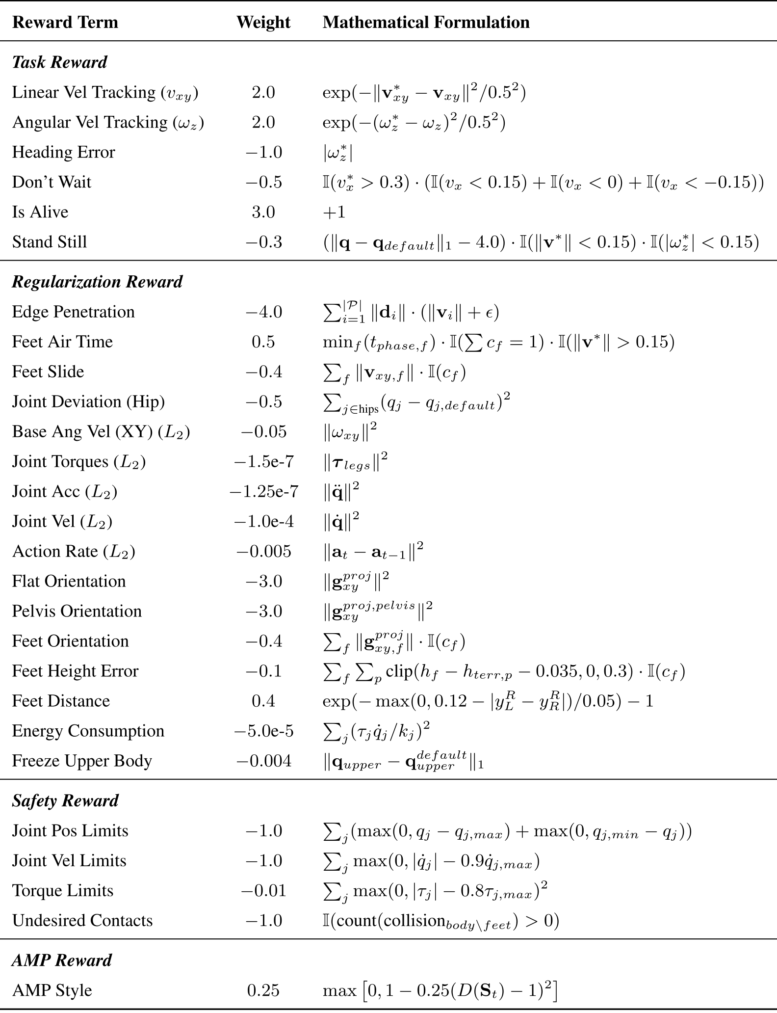
Table 5 preserves all task, regularization, safety and motion-style terms. Velocity tracking has weight 2 for linear and angular targets; edge penetration is −4; staying alive is +3; AMP style is +0.25. The remaining terms regulate waiting, stance, contacts, joint motion, orientation, torque, energy and limits. Reported performance reflects this combined reward design.
Original selectable source
| Reward Term | Weight | Mathematical Formulation |
| Task Reward | ||
| Linear Vel Tracking () | ||
| Angular Vel Tracking () | ||
| Heading Error | ||
| Don’t Wait | ||
| Is Alive | ||
| Stand Still | ||
| Regularization Reward | ||
| Edge Penetration | ||
| Feet Air Time | ||
| Feet Slide | ||
| Joint Deviation (Hip) | ||
| Base Ang Vel (XY) () | ||
| Joint Torques () | ||
| Joint Acc () | ||
| Joint Vel () | ||
| Action Rate () | ||
| Flat Orientation | ||
| Pelvis Orientation | ||
| Feet Orientation | ||
| Feet Height Error | ||
| Feet Distance | ||
| Energy Consumption | ||
| Freeze Upper Body | ||
| Safety Reward | ||
| Joint Pos Limits | ||
| Joint Vel Limits | ||
| Torque Limits | ||
| Undesired Contacts | ||
| AMP Reward | ||
| AMP Style | ||
A.4 Ego-centric Depth Perception Details
Depth synthesis and preprocessing make the policy’s simulated observations resemble the deployed sensor stream.
A.4.1 Efficient Depth Simulation via Parallelized Ray-casting
Cast one ray per pixel and find its first mesh intersection. Convert radial distance into depth along the camera principal axis using the ray-axis dot product (Equations 4–5). This is geometric simulated sensing, not a learned map estimator.
Equations 4–5
| (4) |
| (5) |
A.4.2 Bidirectional Depth Alignment and Noise Modeling
The two domains use different transformations toward a shared observation distribution. Matching that distribution is an engineering objective; the paper does not provide a quantitative distribution-equality test.
Simulation Pipeline ℱ s i m
Crop/resize simulated images, add valid-range Gaussian noise, mask contiguous disparity failures, blur, clip/normalize to [0,1], then occasionally replace the whole observation with noise. The prose names range-dependent noise, while its printed formula uses a single variance within a valid-depth mask. Exact variance, corruption probability and blur settings are not all numerically specified.
Real-world Pipeline ℱ r e a l
Hardware follows aligned crop/resize, invalid-depth inpainting and Gaussian blur. This repairs/smooths the sensor stream; it does not reconstruct a persistent environment map.
A.4.3 Temporal Depth Aggregation via Strided Sampling
The history is frames at t−kℓ−1 for k=0…m−1, including one-frame delay. Eight frames span 7ℓ steps; the appendix leaves the stride ℓ symbolic, so an exact history duration cannot be recovered from the manuscript alone.
Equation 6
| (6) |
A.5 Flat Patch Sampling
Algorithm 1 repeatedly samples xy locations, ray-casts heights within radius 0.2 m and accepts patches whose height range is below 0.05 m. Command gains are kᵥ=kω=2 and the stated numerical epsilon is 10⁻⁶. Flatness checks local support; no explicit connectivity or dynamic-feasibility test appears in the pseudocode.
Original selectable source
A.6 Terrain Configuration
Train on a 10×20 grid of 8×8 m terrains at 0.05 m horizontal/0.005 m vertical resolution, with walls added at probability 0.3. Table 7 retains each geometry, proportion and command range. Running excludes stairs, gaps and several discrete-obstacle categories; Rough (Stand) supplies in-place turning practice.
A.7 Policy Network
A CNN maps depth history to a 128-dimensional embedding through 256-unit projection layers. Concatenate it with proprioception for a four-expert MoE actor–critic: gating width 256, expert widths 256/128/64 and ELU activations. The AMP discriminator uses 1024/512 hidden units. Table 6 retains all listed layer settings.
| Parameter | Value |
|---|---|
| CNN channels | |
| CNN kernel sizes | |
| CNN strides | |
| CNN paddings | |
| CNN pooling | MaxPool |
| Encoder projection units | |
| Encoder embedding dim | |
| Encoder activation | ReLU |
| Policy Type | MoE |
| Number of Experts | |
| Gating hidden units | |
| Expert hidden units | |
| Policy activation | ELU |
| Discriminator hidden units | |
| Discriminator activation | ReLU |
| Terrain Settings | Command Range (walking) | Command Range (run) | |||||
|---|---|---|---|---|---|---|---|
| Terrain Type | Geometric Parameters | Prop. | (m/s) | (rad/s) | Prop. | (m/s) | (rad/s) |
| Rough | Perlin Noise Scale m | ||||||
| Rough (Stand) | Perlin Noise Scale m | ||||||
| Square Gaps | Gap Dist m, Depth m | ||||||
| Stairs Down | Step Height m, Width m | ||||||
| Platform Down | Platform Height m | ||||||
| Stairs Up | Step Height m, Width m | ||||||
| Platform Up | Platform Height m | ||||||
| Discrete Boxes | Height m, Width m | ||||||
| Mesh Boxes | Height Mean m | ||||||
| Slopes | Slope rad | ||||||
A.8 Post-Training for Hardware Deployment
Initialize three hardware-oriented specialists from the general walking checkpoint and train each for another 40,000 simulator iterations on flat plus its target terrain. Walking commands narrow to 0.45–0.55 m/s; running to 1.95–3.05 m/s; lateral velocity remains zero. The general policy is still used for other walking tasks, and policy switching is explicit.
A.9 AMP Training Details
The motion prior supplies style supervision distinct from terrain success rewards.
A.9.1 Reference Dataset Composition
At 50 Hz, walking references combine MPC motions and NOKOV human captures retargeted using GMR, totaling 379.62 seconds. Running uses one 1.54-second LAFAN gait cycle, with symmetric augmentation. Separate training addresses missing walk/run transitions and an imbalanced reference mix. Success with one cycle here does not establish that one cycle suffices for every gait or robot.
A.9.2 Discriminator and Style Reward
The discriminator scores short state sequences. Least-squares targets distinguish reference (+1) from policy (−1) motion, with gradient penalty and weight decay. The clipped quadratic style reward is max(0,1−0.25(D−1)²). Equations 7–8 preserve the exact objective; temporal sequences encourage motion consistency beyond single-frame posture.
Equations 7–8
| (7) |
| (8) |
A.10 Terrain Edge Detector Algorithm
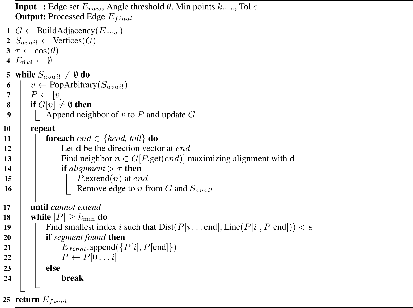
Algorithm 2 identifies adjacent-face edges above the dihedral threshold, processes them, wraps retained segments in cylinders and builds a spatial grid. Algorithm 3 greedily extends aligned connected chains, then approximates them with segments under a distance tolerance. Minimum chain size and greedy ordering affect retained detail; the procedure is not a lossless or optimal global mesh simplification. Threshold values remain symbolic in these algorithms.
Original selectable source
Original selectable source
Appendix B Experiment Configurations
Train 4,096 simulated 29-DOF G1 agents using Isaac Sim/Lab on one RTX 4090. The factory D435i captures 480×270 depth at 60 Hz, downsampled to 64×36 and cropped to 32×18. The Jetson Orin NX runs the policy through ONNX Runtime at 50 Hz while depth preprocessing runs asynchronously.
During deployment, a human supplies velocity commands and uses the stop–stand–switch procedure between policies. The authors’ safety discussion calls for supervision, emergency stop and keeping bystanders outside the operating/fall area; limited recovery prevents interpreting the demonstrations as evidence for unsupervised public operation.
Appendix C Simulation Evaluation Details
Each simulated comparison uses 1,000 parallel agents and one generalist walking policy. Success requires reaching within 0.25 m of the target in 15 seconds without termination. Reaching times average successful trials only, and “–” means no successful trial.
Table 8 specifies challenging test geometry: 0.20 m stair steps, 0.40 m large boxes/platforms, 0.40 rad ramps and 0.60 m gaps, plus roughness and variable small boxes. The 0.60 m simulated gap differs from the reported 0.50 m hardware gap. These terrains are deliberately challenging for the uniform-command baseline; results do not constitute a shared external benchmark.
| Terrain Type | Evaluation Geometry |
|---|---|
| Stair up/down | Step height m |
| Large box | Height m |
| Platform up/down | Platform height m |
| Ramp | Slope rad |
| Gap | Gap distance m |
| Rough terrain | Noise scale |
| Small box | Height m; width and length randomly sampled from m |