Overview
This edition covers the complete ten-page arXiv v1 dated 12 January 2026. Ziwen Zhuang, Shaoting Zhu and Hang Zhao are affiliated with both IIIS, Tsinghua University and Shanghai Qi Zhi Institute; Mengjie Zhao is affiliated with Tsinghua. Hang Zhao is the corresponding author. The missing HTML teaser is restored, and figure numbers follow the PDF.
At a glance
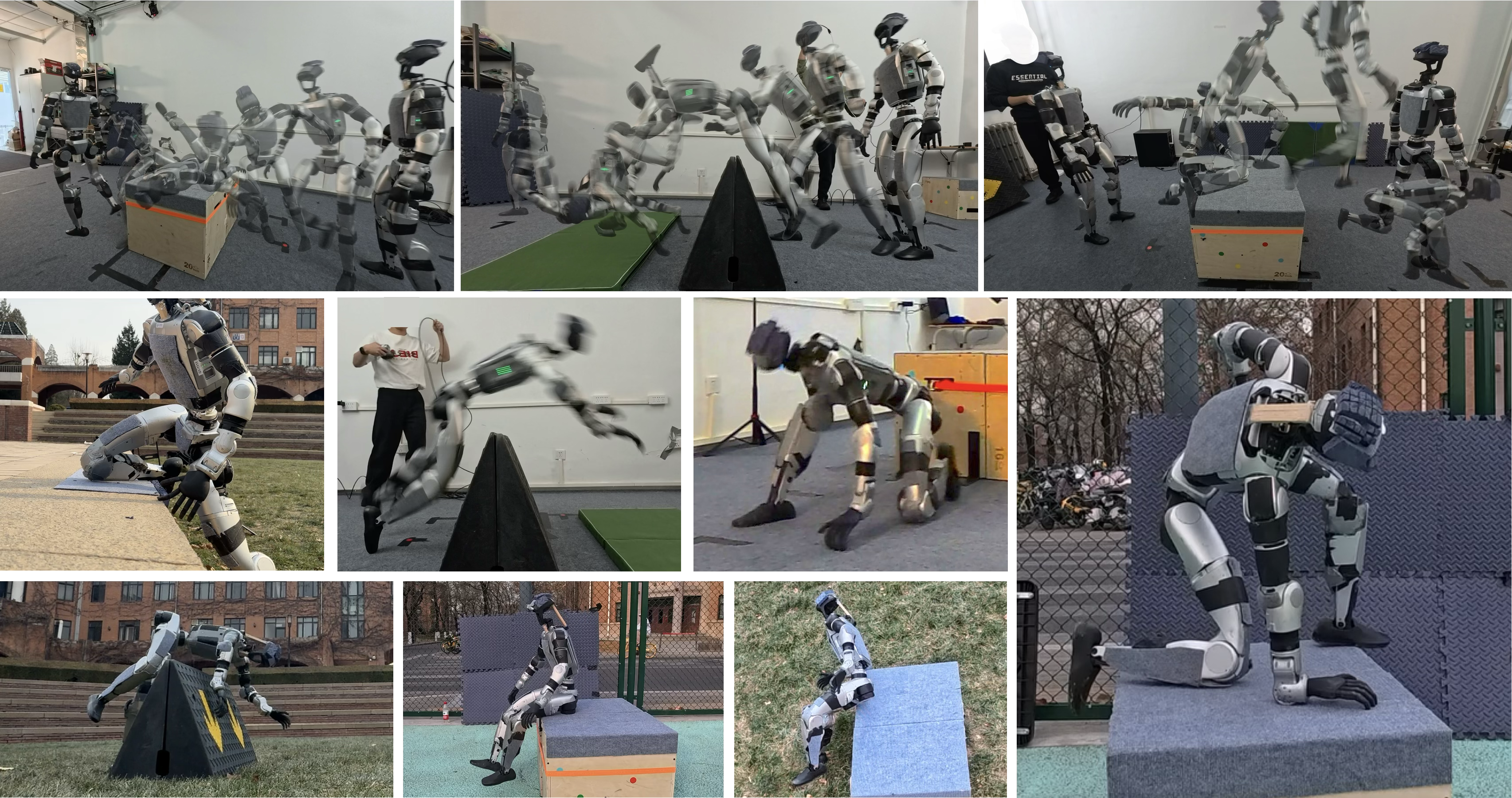
A single humanoid policy combines a selected motion reference with onboard depth sensing. It adjusts whole-body motion to local obstacle geometry, enabling skills such as hand-assisted vaulting and dive-rolling that require more than foot contact.
The study covers four motions across three terrains. Its strongest quantitative evidence is improved global tracking under perturbed starting positions in simulation. Hardware demonstrates indoor and outdoor execution, but supplies no repeated-trial success counts. Operators still choose and trigger the reference skill.
I Introduction
Terrain-aware locomotion anticipates obstacles, while motion imitation supplies rich whole-body task specifications. The proposed controller combines these interfaces: reference motion expresses the intended skill, and depth helps align the robot’s approach and contacts with the obstacle.
This addresses a practical failure of blind playback: correct relative body poses can still put hands or feet in the wrong place globally. The policy uses visual feedback to correct approach position without an external odometry system. This is local adaptation of a supplied skill, not autonomous route planning or skill selection. The original project page is linked in Figure 1.
II Related Works
The related work separates blind locomotion, perceptive locomotion and reference-motion tracking to motivate a controller with both rich motion intent and terrain feedback.
Deep Reinforcement Learning for Legged Control
Proprioceptive history and privileged simulation training support robust legged control. Without exteroception, however, a policy cannot directly observe an upcoming discrete obstacle before contact; reactive stability alone does not specify anticipatory whole-body interaction.
Perceptive Locomotion
Depth and elevation sensing allow anticipatory foot placement. Low-dimensional planar velocity commands do not fully specify whether a humanoid should jump, vault or climb, motivating a richer reference-motion input. The paper’s division is a motivation, not a universal characterization of all prior perceptive controllers.
Data-Driven Humanoid Motion Tracking
DeepMimic and AMP show how motion data can specify expressive physical skills. This work targets the additional problem of aligning those skills to sensed obstacles. Its broad description of prior tracking as planar should not be taken as a proof that every earlier system lacks environmental interaction.
III Method
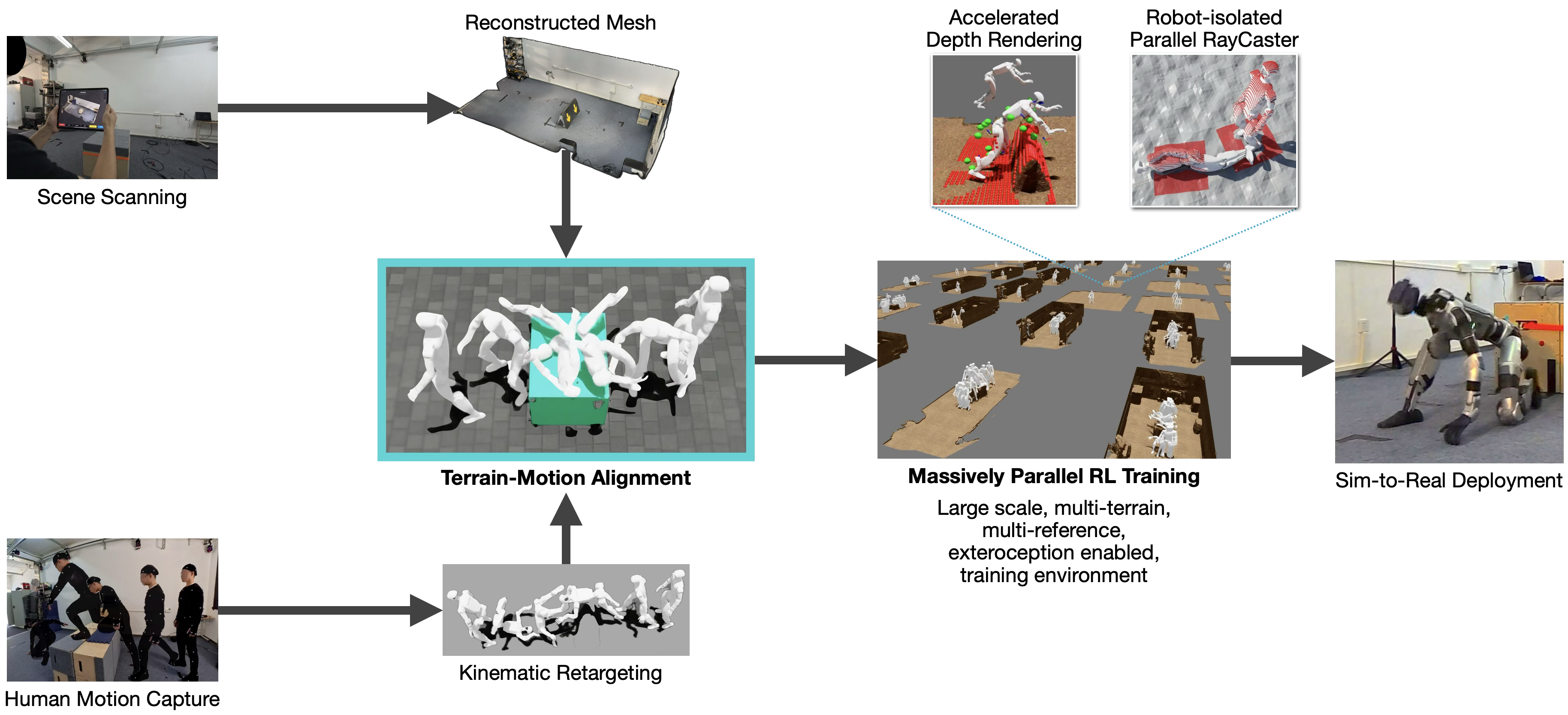
The pipeline pairs human motion with scanned obstacle geometry, trains a depth-conditioned asymmetric actor-critic, then deploys the actor using onboard sensing and reference motion.
III-A Dataset Curation and Environment Generation
Training data must preserve the relationship between body motion and the terrain contacts that make the motion possible.
Motivation and Capture
Unlike general human-motion collections such as AMASS or object-focused OMOMO, this dataset specifically couples parkour demonstrations to large obstacle geometry. Optical motion capture records expert actors while an iPad Pro LiDAR scan reconstructs and aligns the scene. Numbers of actors, clips and total recording duration are not given.
Motion Retargeting
General Motion Retargeting maps human motion to Unitree G1. Optimization-based filtering and manual keyframe edits enforce plausible contacts and suppress capture noise. These kinematic adjustments do not by themselves establish dynamic feasibility; physical tracking is learned afterward.
Procedural Environment Generation
Scans are stripped of laboratory walls, ceilings and incidental context, leaving canonical functional obstacles. Each retargeted motion and its mesh form one paired instance, placed procedurally across an Isaac Lab simulation grid. This varies placement and context, rather than demonstrating unrestricted generalization to new obstacle shapes.
Massively Parallel Ray-Caster for Isolated Multi-Agent Training
A custom Nvidia Warp ray-caster renders depth across parallel robots. Shared mesh prototypes and per-instance transforms reduce duplication. Static terrain belongs to global group −1, while each robot has its own group, preventing other robots’ articulations from appearing in its depth image.
Algorithm 1 precomputes a group-to-mesh hash map. Each ray checks global static meshes and its own robot’s dynamic meshes, instead of searching all mesh groups. The paper reports a 10× rendering gain over a naive baseline but omits timing, hardware and ray-count details. Global static geometry remains visible to every agent, and its intersection work is not constant in the number of static meshes.
III-B Training settings
Training follows the asymmetric actor-critic and tracking-reward ideas of BeyondMimic and VMP. The actor receives deployable observations; the critic also receives simulator pose and terrain information.
Relative Frame
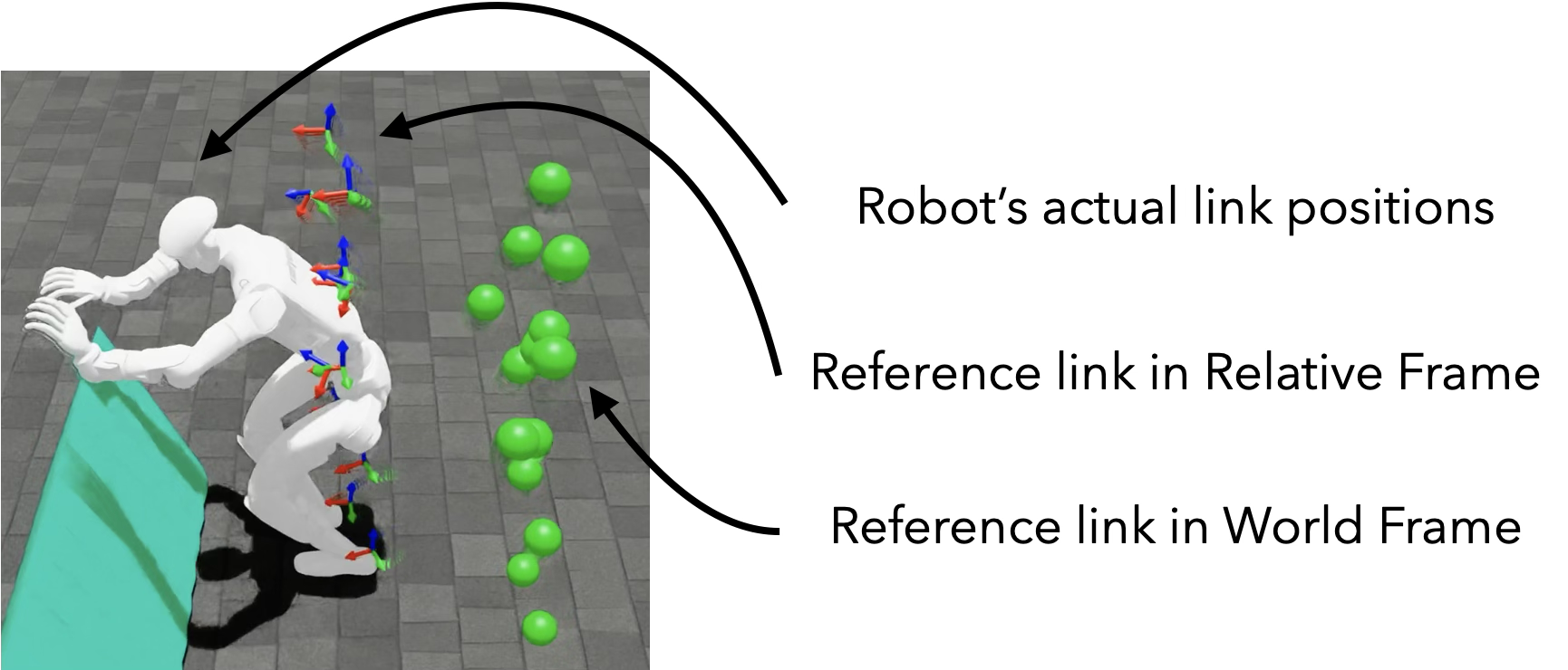
The relative frame takes planar position and yaw from the actual robot, but height, roll and pitch from the reference. The three original equations define its homogeneous transform, translation and rotation composition.
Local pose rewards therefore allow planar approach adjustment while retaining reference tilt and height. Separate global root rewards still compare against the reference using privileged simulator state; odometry-free deployment does not mean training lacks global-position supervision.
Equations
Rewards Definition
Asymmetric PPO uses six tracking terms: global root position and rotation, relative-frame link position and rotation, and world-frame link linear and angular velocity. Penalties cover action changes, joint limits, undesired contacts and torque limits. Rotation errors use axis-angle differences. Reward weights and scales are not supplied.
The actor sees a noisy depth frame, eight proprioception frames and future references. The critic additionally sees actual link transforms and a terrain height scan. The reward subsection includes future root rotation in critic inputs, while the later input list omits it; this source inconsistency is unresolved.
Adaptive Sampling
Algorithm 2 partitions reference motions into bins of at most one second, accumulates failures, smooths neighboring counts and samples future resets in proportion to the resulting weights plus a small positive offset. Difficult motion phases are revisited more often.
The displayed algorithm counts failures without normalizing by visits, so sampling reflects both exposure and difficulty. Kernel parameters, offset and any count forgetting are unspecified. No independent ablation isolates this curriculum’s contribution.
Early Timeout with Stuck Detection
Random resets along a motion can place the robot inside obstacle geometry. A stuck detector truncates episodes that remain trapped near initialization, reducing training on unsolvable rollouts. Detection thresholds and the time limit are not specified.
Network inputs
The actor receives ten future reference samples at 0.1-second spacing, described as a one-second lookahead. These contain joint positions/velocities, reference-relative future base positions and future orientation relative to the actual robot, plus one depth image and eight proprioception frames. No measured global base position is an actor input.
The critic expresses future base positions relative to the actual robot, and adds key-link positions/rotations and a terrain height scan. Privileged critic observations improve value prediction but are not needed by the deployed actor.
Network architecture
A CNN encodes depth and a three-layer MLP combines it with proprioceptive history and reference inputs. The text points to an appendix for detailed parameters, but the supplied ten-page PDF ends with references and has no appendix. Layer widths, depth resolution and full optimization settings cannot be recovered from this manuscript.
III-C Bridging sim-to-real gap in depth perception
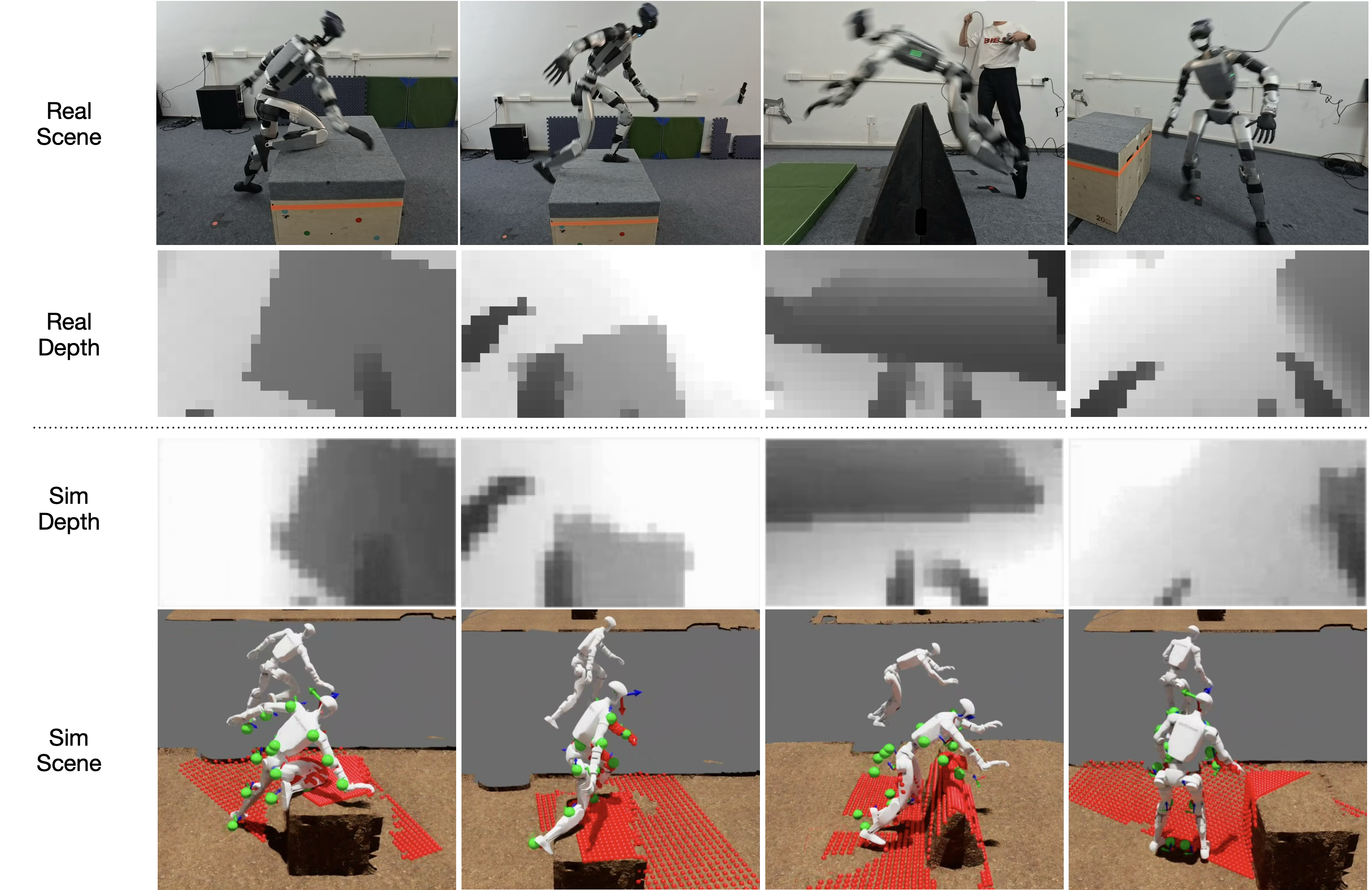
Training uses synchronized depth with Gaussian noise and patch artifacts to mimic reflection, motion blur and stereo failures. RealSense depth runs at 50 Hz; Jetson CPU filtering cannot meet that rate, so deployment uses GPU OpenCV inpainting.
Figure 4 compares simulated and real image patterns. Visual resemblance is not a quantitative sensor-distribution match, and artifact parameters are not provided. The 50-Hz depth rate is not a measured end-to-end control-latency guarantee.
III-D Deployment
A state machine selects the reference motion. ONNX runs neural inference onboard, while camera acquisition and rosbag logging use separate processes and CPU affinity. Reference heading is aligned initially to the robot’s IMU orientation; future orientation is then expressed relative to current orientation.
Reference-relative position inputs avoid dependence on measured global position. This removes external odometry from the actor, while retaining reference selection, initial heading alignment and onboard depth sensing.
IV Experiments
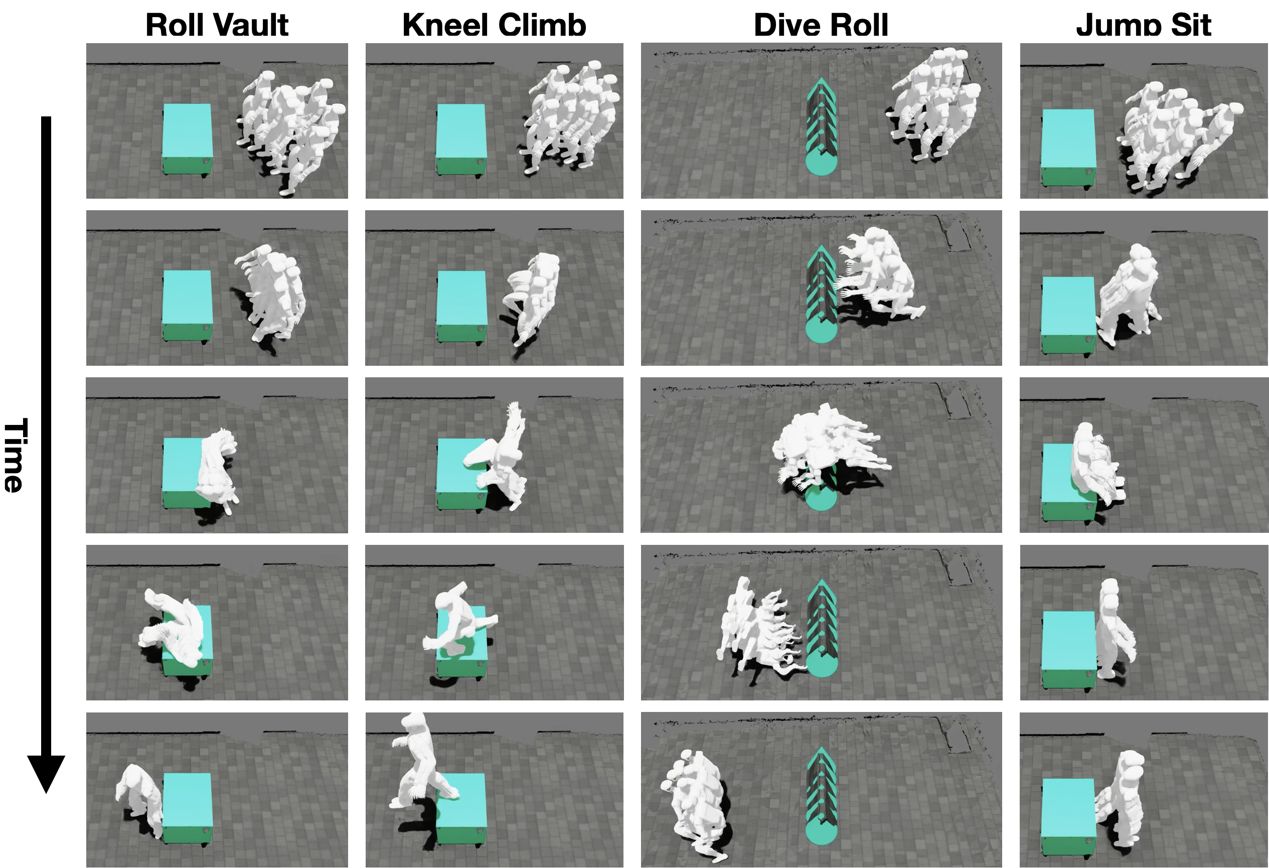
The four skills are kneel climb, roll vault, dive roll and jump sit. Terrains are a triangular barrier made from two road ramps, a 0.5×0.6×0.4-m wooden box, and flat ground. Evaluation asks whether depth improves initial-position tolerance, how distractors affect tracking, and which training ingredients matter.
IV-A Real world experiment
Hardware is a 29-DOF Unitree G1, September 2025 version, with a head-mounted Intel RealSense D435i. ROS 2 coordinates the system and ONNX inference uses the onboard CPU. An operator walks the robot to a rough start and triggers a specific reference; the controller returns to walking when the reference ends.
Indoor tests collect wired logs; outdoor demonstrations do not use the additional logging system. No accurate global localization is required, but skill choice and triggering remain manual. The paper reports no hardware trial counts, confidence intervals or quantitative success rates.
IV-B Non-trivial benefit of depth vision
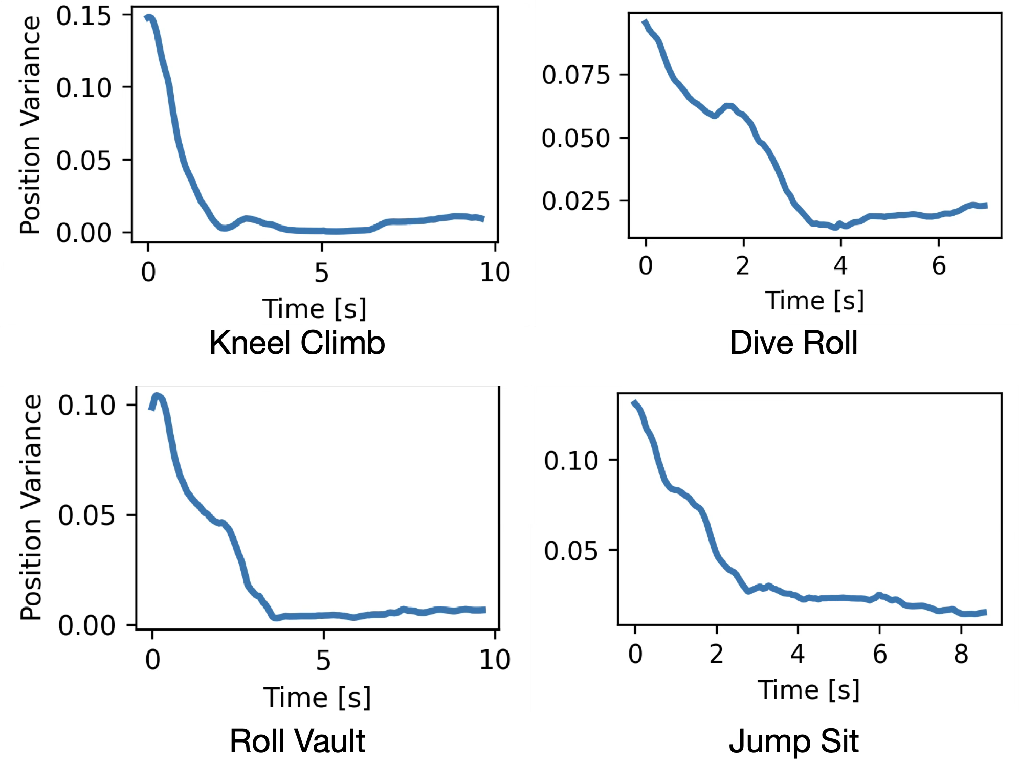
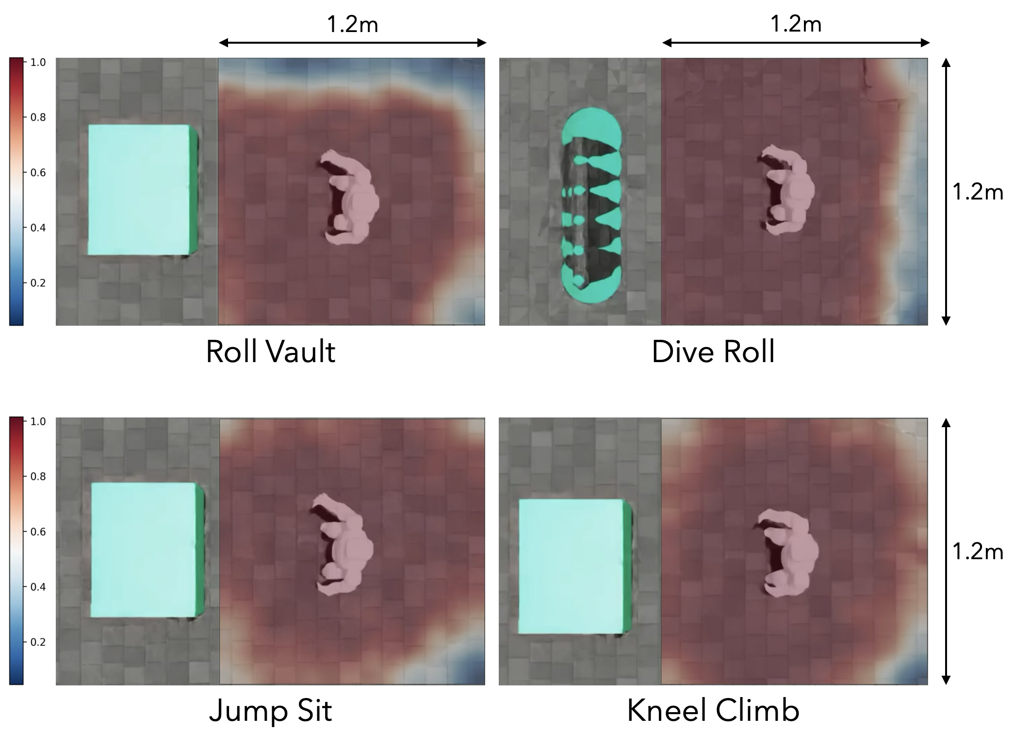
Training randomizes initial x/y within ±0.15 m. A convergence example tests a 0.5×0.5-m region; broader heatmaps cover ±0.6 m on each axis. Figure 5 shows position variance shrinking during approach and sometimes rising late as depth features become less distinctive.
With position randomization, the full model reduces global mean per-joint position error against the blind baseline from 0.2267 to 0.1649 for dive roll, 0.1822 to 0.1218 for kneel climb, 0.1969 to 0.1421 for roll vault and 0.2693 to 0.1446 for jump sit. Base-relative errors do not improve uniformly, and table units are not explicitly stated.
Figure 6 shows skill-dependent success regions, including failures near their boundaries; it does not establish 100% success throughout the 1.2-m square. Trials per cell and the exact completion criterion are not specified. Without position randomization, depth is also not uniformly better on global or local tracking error.
| Training Variant | Dive Roll | Kneel Climb | Roll Vault | Jump Sit | ||||
|---|---|---|---|---|---|---|---|---|
| Testing with no position randomization | ||||||||
| w/o depth (BeyondMimic) | 0.1365 | 0.0462 | 0.1162 | 0.0378 | 0.1109 | 0.0358 | 0.1909 | 0.0341 |
| w/o stuck detection | 0.1367 | 0.0464 | 0.1073 | 0.0394 | 0.1162 | 0.0393 | 0.1170 | 0.0389 |
| local frame reward | 0.1213 | 0.0242 | 0.1145 | 0.0383 | 0.1131 | 0.0332 | 0.1358 | 0.0299 |
| ours | 0.1468 | 0.0459 | 0.1063 | 0.0388 | 0.1123 | 0.0351 | 0.1197 | 0.0362 |
| Testing with position randomization | ||||||||
| w/o depth (BeyondMimic) | 0.2267 | 0.0477 | 0.1822 | 0.0405 | 0.1969 | 0.0385 | 0.2693 | 0.0377 |
| w/o stuck detection | 0.1661 | 0.0456 | 0.1449 | 0.0412 | 0.1461 | 0.0316 | 0.1322 | 0.0354 |
| local frame reward | 0.1892 | 0.0389 | 0.1477 | 0.0402 | 0.1453 | 0.0311 | 0.1312 | 0.0301 |
| ours | 0.1649 | 0.0477 | 0.1218 | 0.0399 | 0.1421 | 0.0371 | 0.1446 | 0.0382 |
IV-C Vision robustness
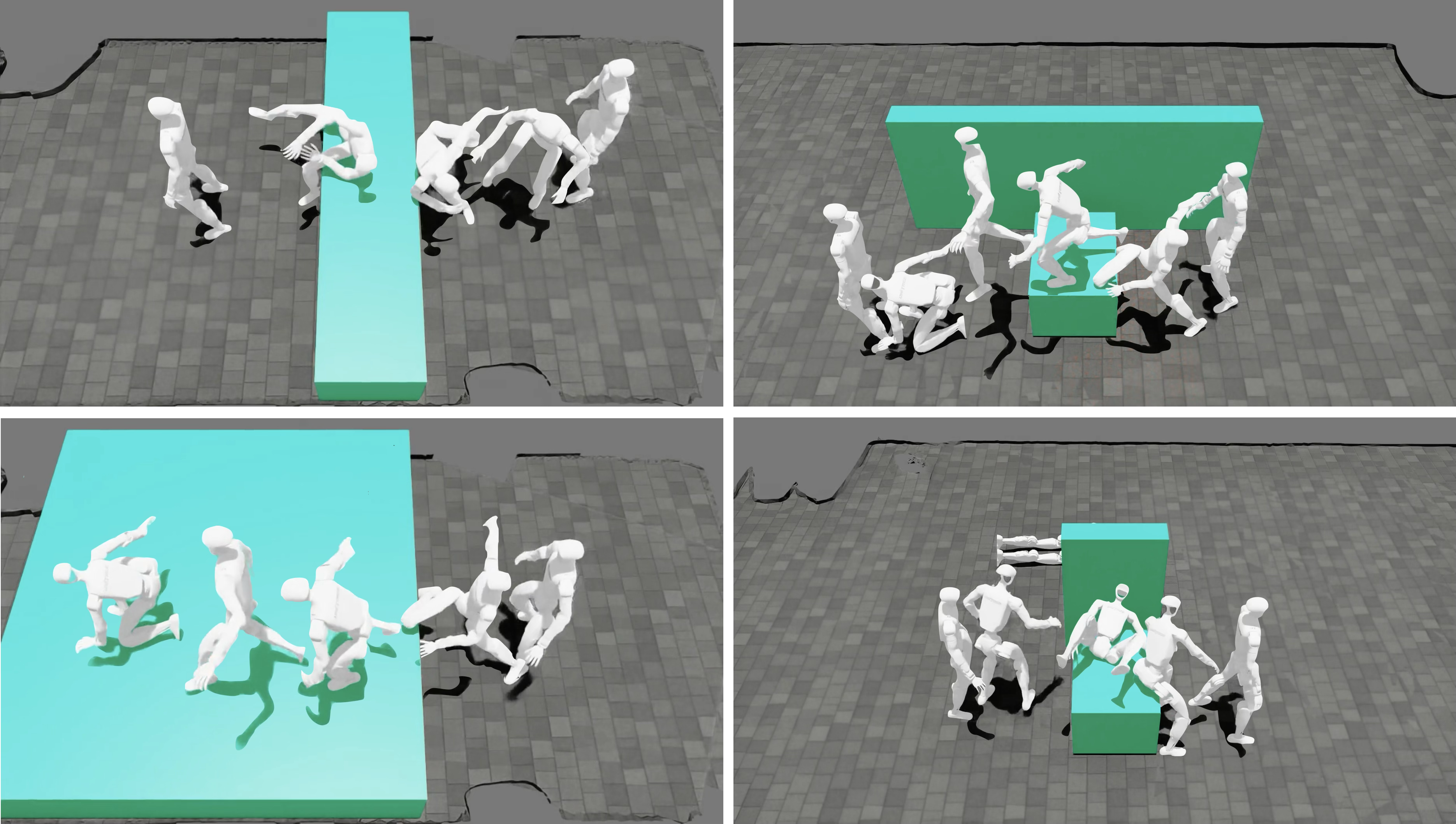
Two motions are tested with wide, plane and wall distractors, alongside the original scene. The stated protocol uses batches of 100 simulated robots without initial-position randomization. The plane can alter physical interaction as well as visual input, so this is not a purely visual robustness test.
The authors report no observed success-rate drop but give no numerical completion totals. Tracking precision can worsen sharply: kneel-climb global error rises from 0.1022 to 0.4848 with the wide distractor, and roll-vault global error rises from 0.1159 to 0.5598 with the plane. Completion robustness and precise reference tracking are different outcomes.
| Distractor Condition | Kneel Climb | Roll Vault | ||
|---|---|---|---|---|
| No Distractor | 0.1022 | 0.0390 | 0.1159 | 0.0349 |
| Wide Distractor | 0.4848 | 0.0405 | 0.1543 | 0.0373 |
| Plane Distractor | 0.4261 | 0.0417 | 0.5598 | 0.0809 |
| Wall Distractor | 0.1603 | 0.0401 | 0.1157 | 0.0372 |
IV-D Ablation on the training recipe
Table I compares depth removal, stuck-detection removal and replacing the mixed relative frame with the robot’s local frame. Depth most consistently improves global tracking when starts are perturbed. The relative frame improves global error for three skills against the local-frame variant, but jump sit favors the local frame.
Stuck detection reduces wasted impossible resets, yet its error advantage is mixed: without it, randomized jump-sit global error is 0.1322 versus 0.1446 for the full model. These results support specific design choices under particular conditions, not a uniform win on every motion and metric.
V Conclusion
Combining selected motion intent with onboard depth enables contact-rich humanoid skills and reduces dependence on exact starting placement. The demonstrated scope remains four motions, three terrain types and limited quantitative simulation tests.
Scaling motion data and selecting skills autonomously are future work. Missing training parameters, unquantified hardware reliability, depth artifacts and distractor-induced tracking errors limit reproduction and broader deployment claims.
Acknowledgments
The authors acknowledge Xiangting Meng, Siqiao Huang, Yizhuo Gao and Tairan He.