Overview
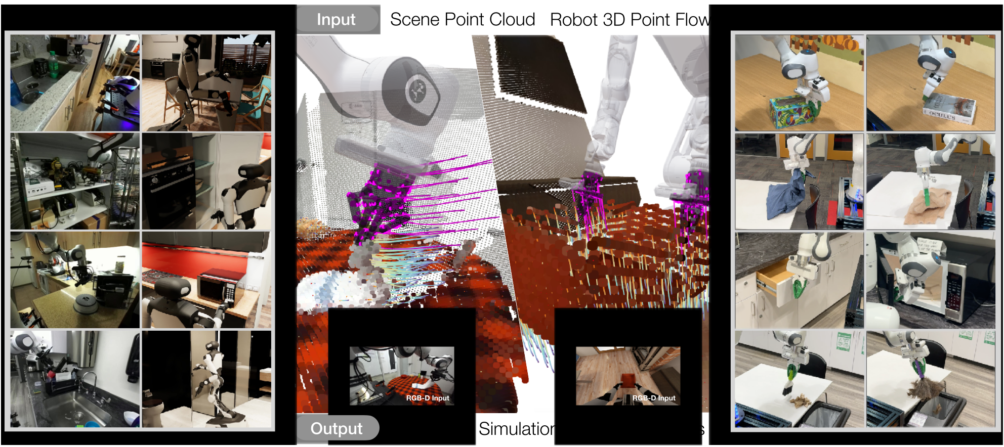
PointWorld predicts how observed scene points move when a robot follows a proposed geometric trajectory. Its shared point-flow representation supports several robot embodiments, while a sampling planner uses the predicted motion to select actions.
At a glance
A large point-cloud dynamics model learns from real DROID demonstrations and simulated BEHAVIOR-1K interactions, totaling roughly two million clips and 500 hours after curation. Modern point-cloud backbones, pretrained image features, movement-weighted robust losses and chunked prediction improve short-horizon flow accuracy. A pretrained model supports eight physical manipulation tasks with manually specified goals; these trials execute a single optimized plan without visual replanning.
1 Introduction
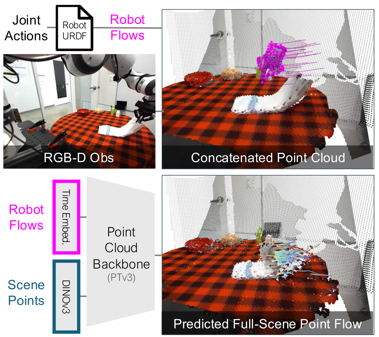
Represent both the environment and the robot’s intended motion in the same 3D space. RGB-D supplies partially observed scene geometry; known robot kinematics supplies fully specified action geometry. Predicting their interaction avoids encoding each embodiment through a different joint/action vector and focuses learning on motion rather than photorealistic appearance.
This edition covers all 38 pages of arXiv v1, dated 7 January 2026, with all seven authors verified. The catalog’s CVPR 2026 publication metadata is retained. The core evidence concerns one-second geometric prediction, transfer between the reported domains, and selected physical tasks, rather than unrestricted physical simulation or general autonomous task specification.
2 Related Work
The representation sits between image-based world models and explicit physics simulators: it learns the motion of observed geometry without requiring a complete object/material decomposition.
World Modeling.
World models may predict pixels, latent features, meshes, radiance fields or particles under various action interfaces. PointWorld uses 3D point flows for both state and action, emphasizing contact geometry and allowing single-pass regression rather than iterative video generation.
Dynamics Models in Robotics.
Analytical simulators encode physical assumptions explicitly; learned dynamics models fit interactions from data and can support planning or policy learning. PointWorld extends particle-style learned dynamics, a family covered by the cited dynamics-model review, toward larger datasets and heterogeneous embodiments, without claiming exact physics laws.
2D and 3D Flows for Manipulation.
Prior flow methods provide representations for policies, goals, rewards or visual servoing. Here, FoundationStereo, VGGT and CoTracker3 construct 3D training supervision, while known robot geometry converts proposed actions to point trajectories.
3 Method
First learn action-conditioned scene motion; then optimize candidate robot trajectories using that learned forward model. The dynamics network itself neither chooses a task nor guarantees an executable robot trajectory.
3.1 3D World Modeling with PointWorld
A single forward pass predicts ten future steps spaced 0.1 seconds apart. This one-second chunk preserves temporal relationships while amortizing the point-cloud backbone across multiple future states.
State Representation.
Remove robot pixels using its URDF and current joints, then back-project the remaining calibrated RGB-D observations into scene points. Point identity is maintained within the imagined rollout. No online point tracker is required at inference, and the initial point set can change between observations. A static initial cloud does not encode initial object velocity.
Action Representation.
Sample surface points on robot links and propagate them through the proposed joint sequence using forward kinematics. Unlike partially visible scene points, the robot action geometry is known even behind an object. Most experiments retain only 300–500 gripper points; assuming the robot actually follows this forecast is distinct from modeling actuation/contact-induced tracking error.
Dynamics Prediction.
Concatenate initial scene points with time-stacked robot points. A Point Transformer V3 backbone processes the cloud; a shared MLP predicts each scene point’s displacement at all ten steps. Frozen DINOv3 image features are projected onto scene points, and robot features carry temporal information. The roughly 0.1-second forward-pass figure excludes the complete iterative planning procedure.
Training Objective.
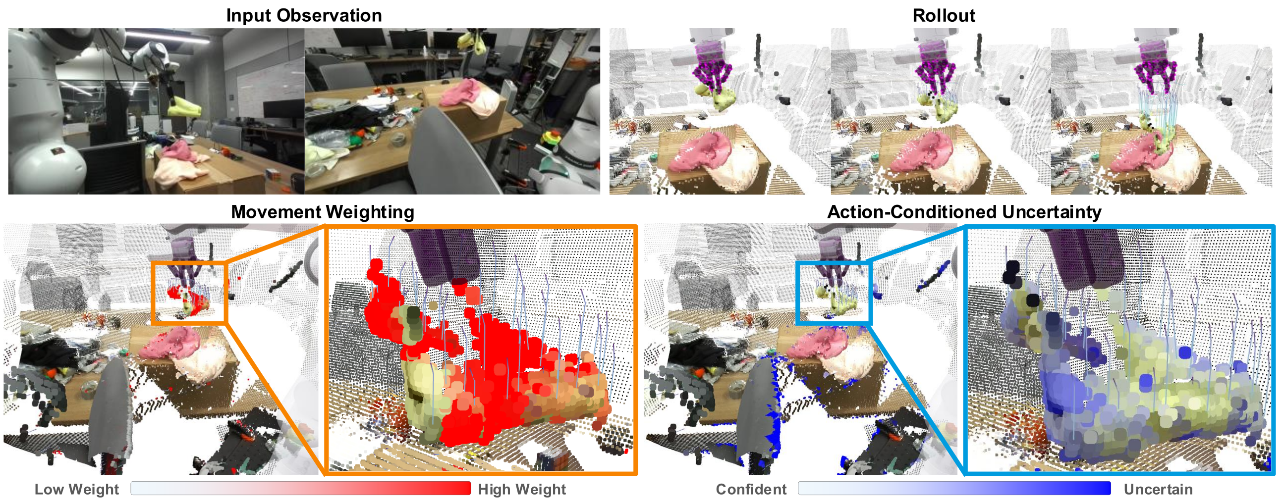
Most scene points remain still, so uniform regression can neglect contacts. A sigmoid of ground-truth displacement assigns movement weights, normalized across points and timesteps. Huber residuals and predicted log-variance reduce the influence of unreliable real-world tracks (Equation 1). Visibility/depth-invalid labels receive no supervision.
Movement weighting alone can emphasize noisy outliers. The uncertainty and robust-loss terms stabilize it; learned uncertainty is not a demonstrated calibration guarantee or a separation of physical randomness from annotation noise.
Equation 1
| (1) |
3.2 PointWorld for Robotic Manipulation
MPPI samples temporally correlated end-effector trajectories, converts them to robot flows, predicts the resulting scene, and updates a nominal trajectory using exponentiated negative costs. Task cost is mean squared distance between selected scene points and target positions; control penalties limit path length and poor reachability.
The formulation can support receding-horizon control, but Appendix A.6 explicitly says the reported robot trials do not replan. Goals are manually selected through a GUI; language-model goal generation is a proposed extension. No deployment demonstrations or task-specific model fine-tuning are used.
Equation 2
| (2) | ||||
4 Dataset Curation and Evaluation Protocol
The dataset combines reconstructed real interactions and exact simulator trajectories. Its approximately two million training trajectories are short, overlapping clips rather than two million independent complete demonstrations.
3D Annotation for Real-World Data.
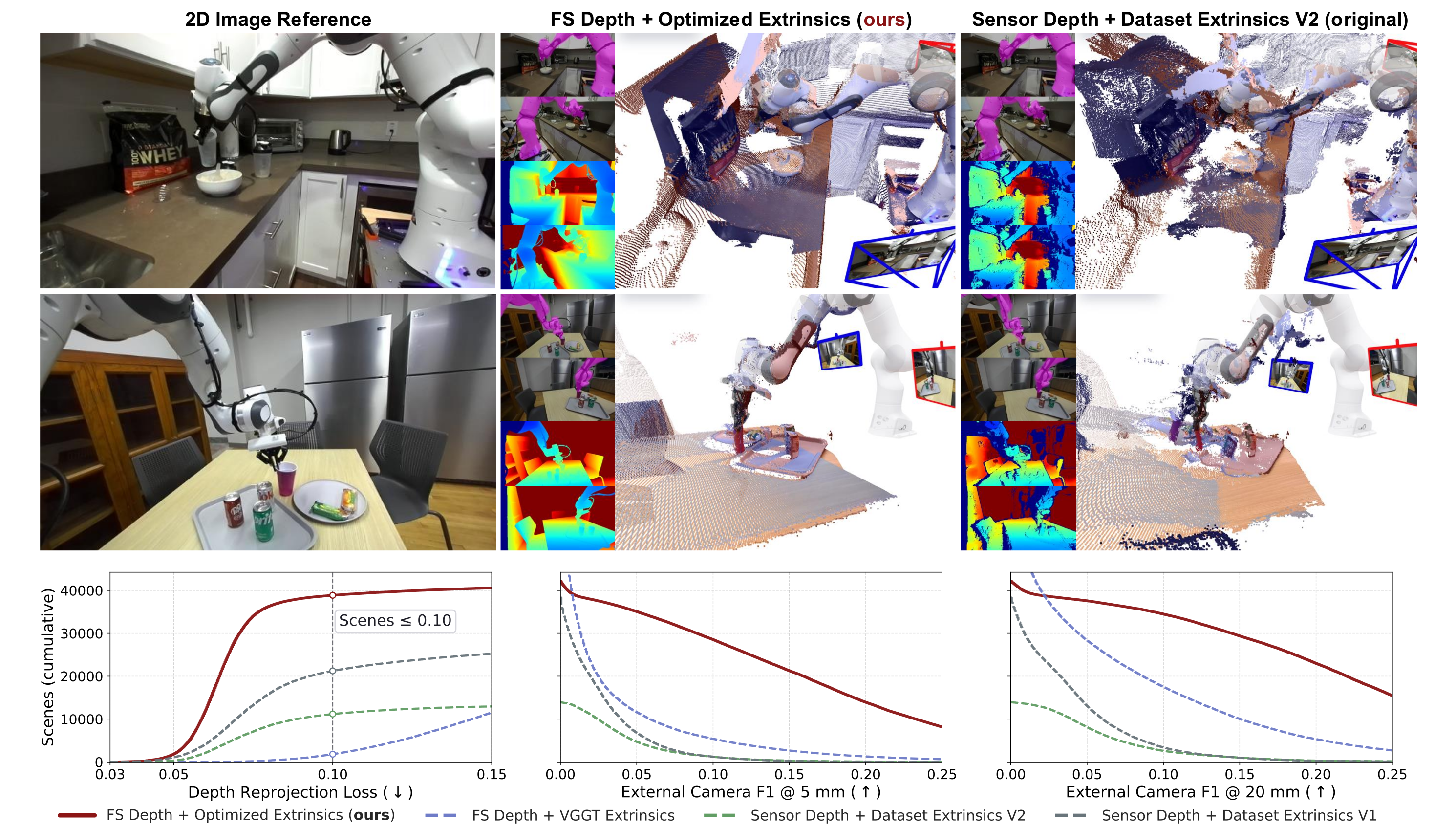
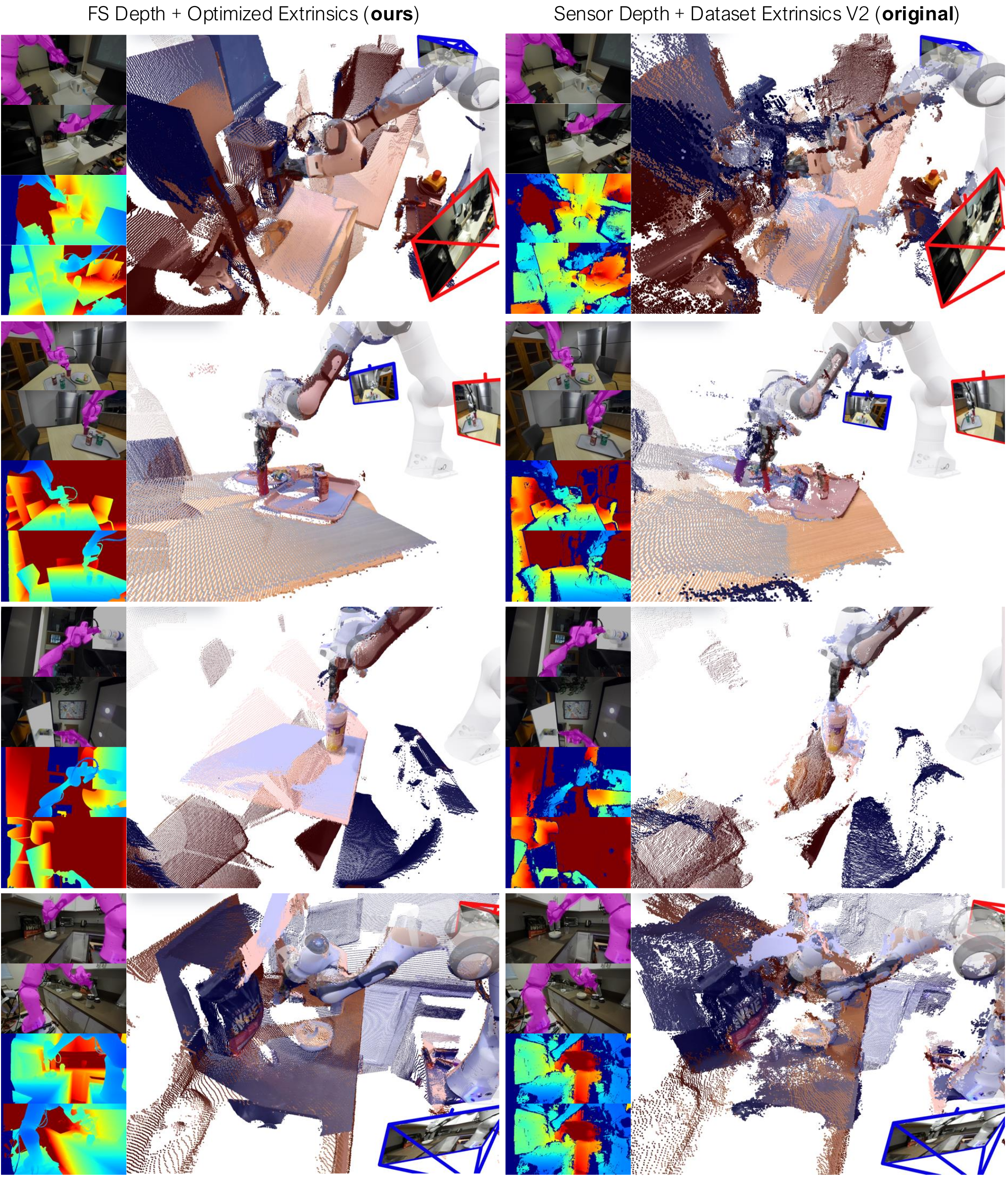
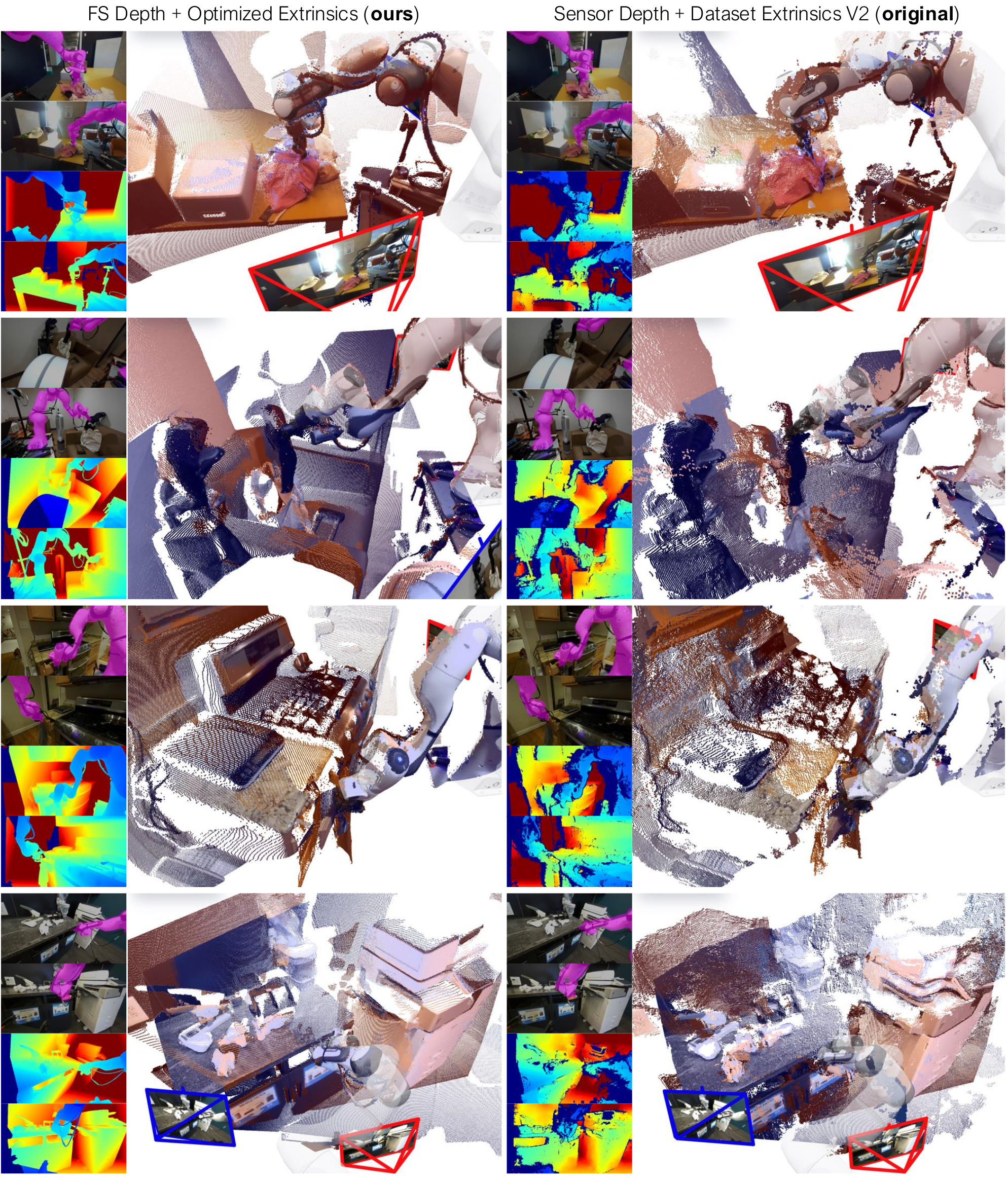
DROID supplies single-arm teleoperation with two external cameras and a wrist camera. Replace sensor depth with FoundationStereo, initialize extrinsics with VGGT, refine them using known robot geometry, and lift CoTracker3 tracks into 3D. The pipeline recovers about 60% of DROID, nearly 200 hours, with visibly improved alignment.
Reported median extrinsic differences of 1.8 cm and 1.9° use the best 1% of original calibrations as a reference proxy, not independently measured ground truth. Figure 5 compares depth consistency and cross-view alignment; missing inputs can change the number of evaluated scenes.
Simulation (BEHAVIOR-1K).
BEHAVIOR-1K contributes Galaxea R1 Pro mobile bimanual interactions from about 1,100 hours before filtering. Replay simulator state to obtain exact link motion and scene flows. Filtering emphasizes interactions but also retains robot-motion/no-object-motion negatives, a detail more explicit in the appendix than the main text’s contact-only description.
Model Evaluation Protocol.
Report per-point, per-timestep Euclidean displacement error, especially on moving points. Simulation uses exact labels. DROID uses a separate expert trained on the evaluation split only to create shared confidence masks; evaluated dynamics models train on the training split. These are filtered-label errors, not measurements against a fully clean independent ground-truth sensor.
The main text says it keeps the top 80% of points by confidence, whereas Appendix A.5 rejects points below the 0.8 confidence quantile, which would ordinarily keep roughly 20% before voxel aggregation. This unresolved source discrepancy affects the metric’s population.
Interpretation of the Metric.
Errors average over one-second horizons and many points; small changes can alter rollout quality. The claimed standard error ≤10⁻⁵ m reflects this dense evaluation, not an uncertainty bound on physical task success. Points within a clip and overlapping clips are correlated. Mover error, static error and deployment success answer different questions.
5 Experiments
Controlled comparisons examine backbones, objectives, image features, model/data size, action representation, rollout strategy, view count and transfer. Physical planning is evaluated separately from prediction accuracy.
Backbone
Params
Mem.
FLOPs
Latency
mov.
stat.
❍ GBND
0.0390
0.0066
❍ PointNet
0.0369
0.0084
❍ PointNet++
0.0368
0.0073
❍ SparseConv
0.0396
0.0076
❍ Transformer
0.0339
0.0071
⚫ PTv3-50M
0.0331
0.0067
⚫ PTv3-132M
0.0324
0.0061
⚫ PTv3-411M
0.0315
0.0059
⚫ PTv3-1B
0.0312
0.0056
5.1 Scaling 3D World Models: A Roadmap
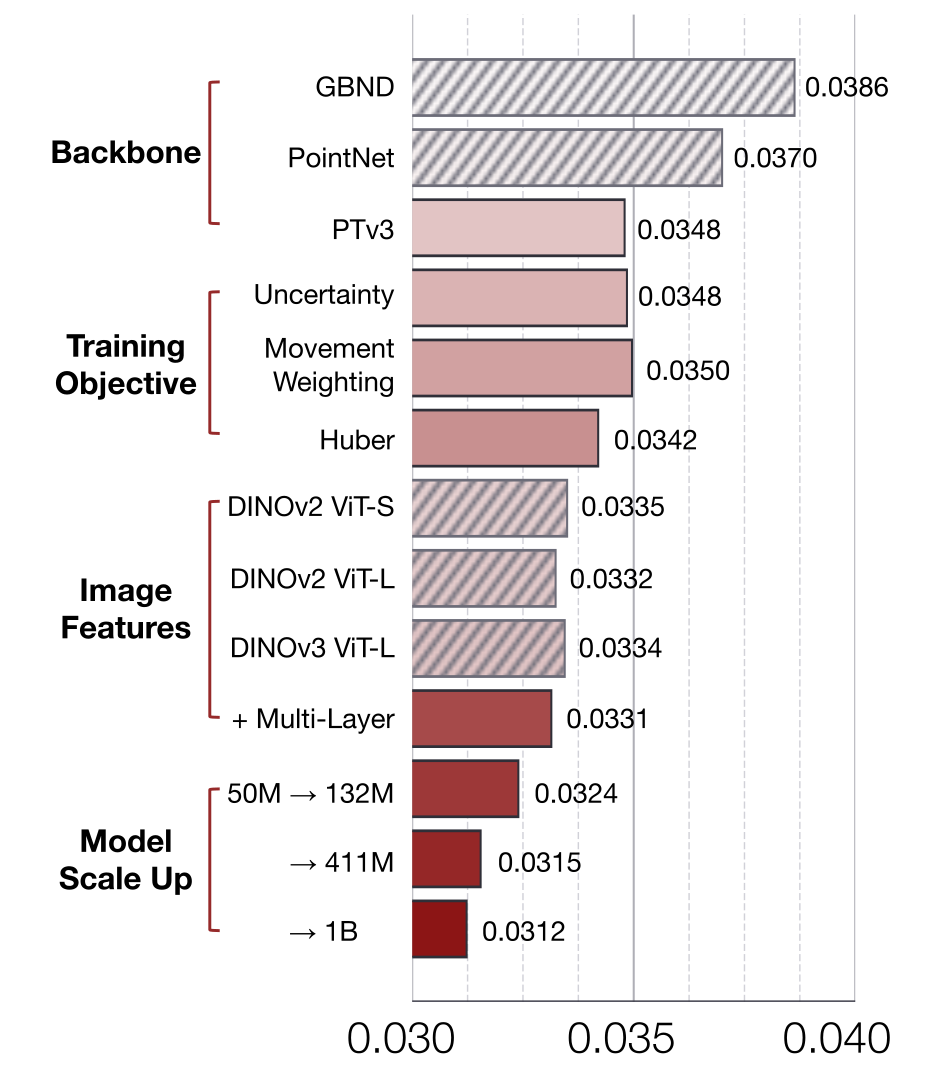
PTv3 scales to about 957 times the GBND baseline’s parameters with 4.30 times its memory in Table 1. The 1B variant has 123.65 ms latency and mover/static errors of 0.0312/0.0056 m. Larger parameter count alone is not a latency improvement over the smaller baseline.
Figure 7 progressively adds a modern backbone, robust objectives, pretrained image features and capacity. Movement weighting initially worsens error without stabilization. Multi-layer frozen DINOv3 features and larger models produce further gains; the roadmap is sequential, so it does not isolate every possible interaction between changes.
| In-Domain | Cross-Domain | Held-Out Real | From | ||||||
| Scratch | |||||||||
| Zero-Shot | mover | 0.0315 | 0.0087 | 0.1460 | 0.0558 | 0.0305 | 0.0531 | 0.0300 | 0.0293 |
| static | 0.0059 | 0.0010 | 0.0050 | 0.0058 | 0.0049 | 0.0057 | 0.0063 | 0.0043 | |
| Finetuned | mover | – | – | 0.0107 | 0.0378 | 0.0271 | 0.0299 | 0.0272 | 0.0293 |
| static | – | – | 0.0003 | 0.0086 | 0.0040 | 0.0046 | 0.0040 | 0.0043 | |
5.2 Ablations
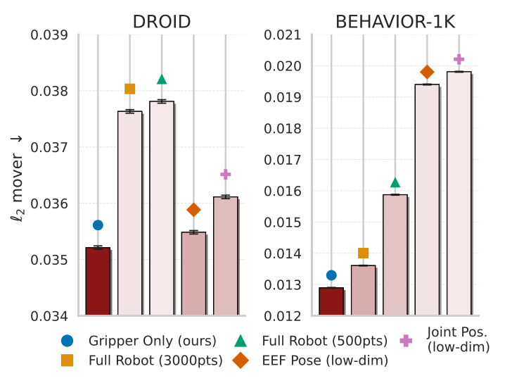
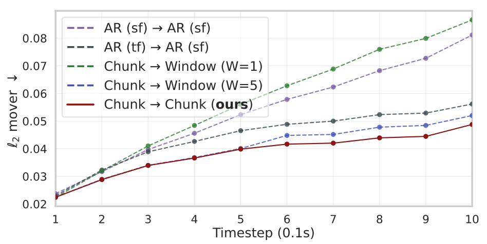
Action geometry: gripper-only flows outperform sparse whole-body flows, dense whole-body flows and low-dimensional joint/end-effector inputs across the tested domains. Dense robot clouds add computation and many non-contact points. Prediction: train/test chunks of ten steps drift less than teacher-forced, self-fed or short sliding-window alternatives and need fewer forward passes.
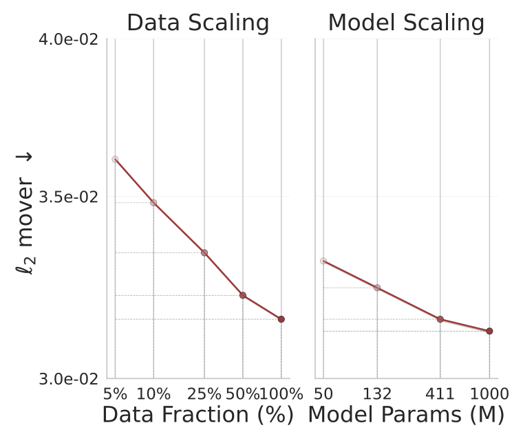
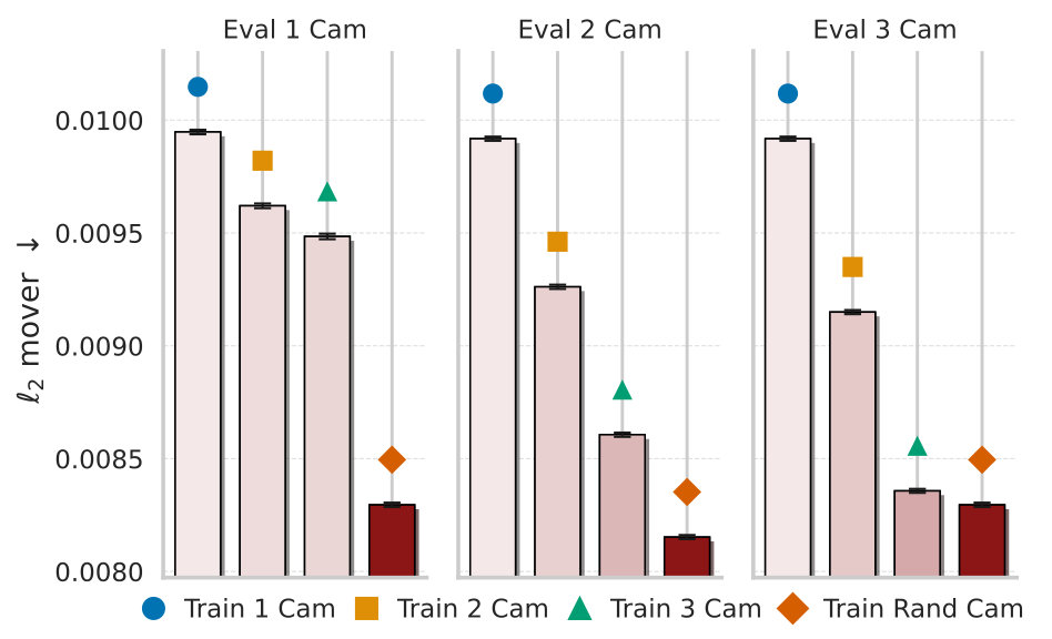
Views: randomizing one to three training views gives the strongest robustness across tested camera counts; added test cameras help. Figure 13 reports sub-centimeter mover errors for that experiment, which should not be conflated with Table 1’s approximately three-centimeter DROID mover errors. Scaling: varying 50M–1B parameters or 5–100% data separately produces approximately log-linear gains within the measured range, not a universal extrapolation law.
The dense whole-body baseline is described as 2,000 points in the prose but labeled 3,000 points in Figure 11; the original figure is retained without silently choosing between them.
5.3 Generalization and Transfer
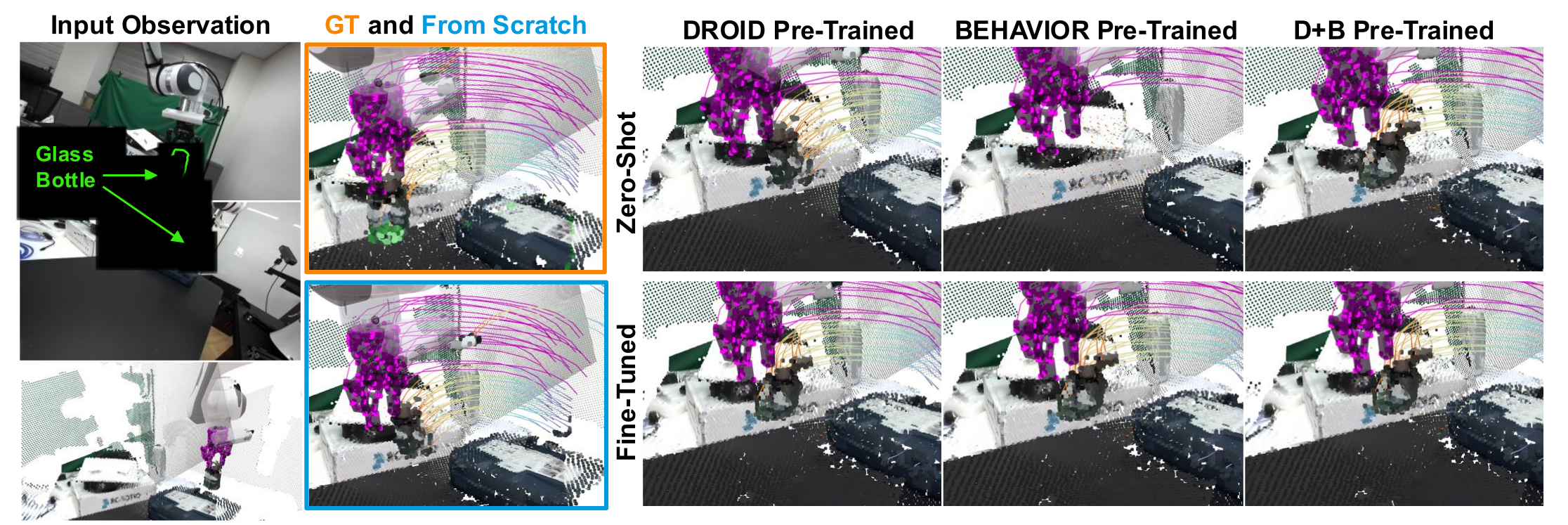
Table 2 separates in-domain, cross-domain and held-out-lab tests. On the held-out lab, real-only and joint real/simulation pretraining yield zero-shot mover errors of 0.0305 and 0.0300 m, close to the from-scratch specialist’s 0.0293 m. Simulation-only pretraining gives 0.0531 m.
Fine-tuning uses 90% of the held-out lab data and evaluates on the remaining 10%. Its 1/20 training updates is a compute/update reduction, not evidence of twentyfold fewer training examples. Fine-tuned real/joint models reach 0.0271/0.0272 m, beating the specialist in this table; simulation-only reaches 0.0299 m. Real-to-simulation transfer improves more readily than simulation-to-real.
5.4 Model-Based Planning with PointWorld
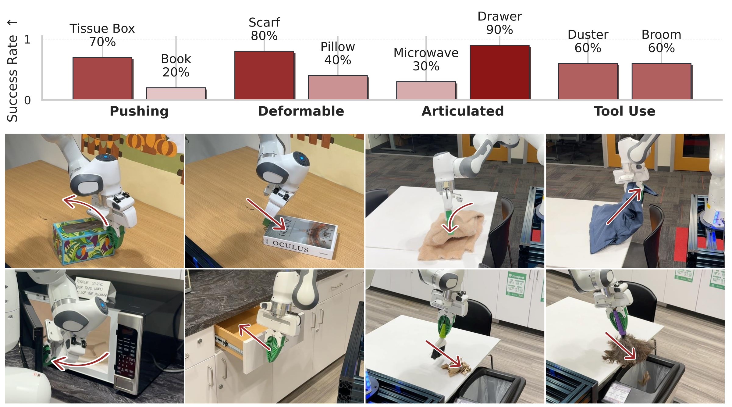
A Franka arm with an unseen fin-ray gripper plans from one RealSense capture and manually selected object targets. Figure 8 reports tissue-box push 7/10, book push 2/10, scarf fold 8/10, pillow placement 4/10, microwave opening 3/10, drawer closing 9/10, duster sweeping 6/10 and broom sweeping 6/10.
Those counts sum to 45/80 successes, calculated from the figure. Each task has only ten feasible initial configurations; there is no reported competing physical-controller baseline. Deformable and tool tasks start pre-grasped. The trials demonstrate varied transfer, while manual goals, one-shot execution and limited sample sizes constrain broader autonomy/reliability claims.
6 Conclusion
The contribution is a scalable geometric dynamics representation plus data curation and training practices that support transfer. Broader generalization remains limited by missing initial velocities, noisy perception, robot tracking assumptions and manual objectives. The paper promises code/data/checkpoints; their availability and usability are not independently evaluated here.
Acknowledgments
The authors acknowledge Stanford HAI, Schmidt Sciences and ONR support, plus colleagues who helped with discussion, data, experiments and feedback.
Appendix A Appendix
The appendix supplies limitations, data construction, training and evaluation details, physical-trial protocol and additional visual evidence.
Appendix Contents
All appendix subsections, eight numbered tables, thirteen displayed equation containers and the complete figure series are retained below.
A.1 Extended Discussions on Limitations
These limitations define the scope of the learned forward model and distinguish observed short-horizon transfer from general physical understanding.
Static Initial State.
The initial observation contains no motion history or object velocity. The formulation assumes a static initial scene; fully dynamic starting conditions would need tracked history or recurrent state.
Reward/Cost Specification for Action Inference.
Action optimization needs an explicit reward/cost. Reported tasks use manual point masks and goals. VLM-based goals, learned rewards and policies trained inside the model are future possibilities rather than tested substitutes here.
Fine-Scale Objects and Calibration Noise.
Depth/extrinsic error can be comparable to the width of pens or cables, confusing object and gripper tracks. Better calibration/annotation is needed for fine-scale contact supervision.
Correlation vs. Causation.
Training captures correlations among robot actions, motion and observed change. Exogenous influences are not disentangled as causal mechanisms; good conditional prediction does not prove causal identification.
Lack of Photometric Dynamics.
Predicted outputs move observed 3D points; they do not model lights turning on, screen changes or appearance evolution. A separate appearance/radiance model would be needed.
Rigid-Body Robot Assumption.
Forward kinematics treats the robot as rigid links. Compliance in a fin-ray gripper and other contact-induced deformation are not explicitly represented, even though the deployment gripper is compliant.
Actuation and Tracking Assumptions.
The network predicts scene consequences if the robot follows the supplied path. It does not jointly model whether motor limits, payload, contacts or tracking error will prevent that path from being realized.
Lack of Explicit Physics Priors.
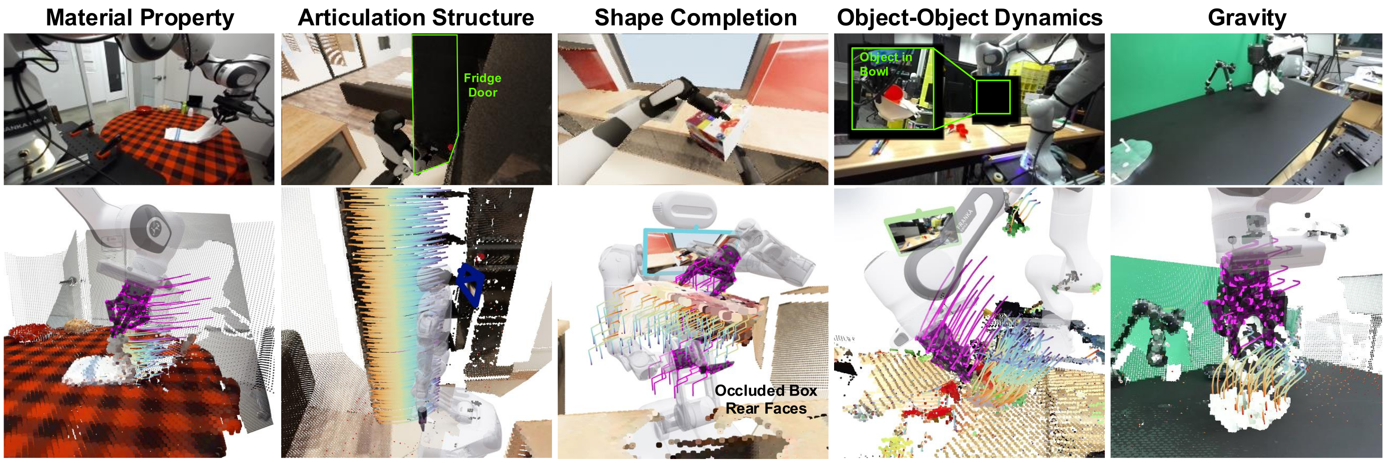
No Newtonian/conservation constraints are imposed. Qualitative gravity, articulation and deformation behavior emerges from data, without a guarantee of physical consistency outside the training distribution.
A.2 DROID 3D Annotation Pipeline
Real-data preprocessing reconstructs geometry and trajectories from synchronized stereo views and recorded joints, regardless of demonstration success. Robot geometry includes the Robotiq 2F-85 gripper and custom camera mount; model inputs ultimately use the external views.
A.2.1 Depth Estimation
FoundationStereo estimates per-view metric depth. Clip to a trusted 0–4 m range and propagate validity masks. This differs from simply accepting the original sensor depth or assuming a near-field stereo cutoff.
A.2.2 Camera Pose Estimation
Estimate one rigid transform per external camera and scene. Use multi-view initialization, then optimize against visible robot geometry whose pose is known from joints.
Camera Pose Initialization.
VGGT estimates time-aligned wrist/external camera relations. Known wrist-to-gripper calibration and forward kinematics tie these to the robot base; averaging over valid wrist frames initializes the external transforms. The displayed formulas retain the original coordinate-frame directions.
Equations
Camera Pose Refinement.
Refine six-DOF external-camera updates using absolute robot-depth reprojection error. Run 100 steps at learning rate 10⁻³, trust robot depths of 0.3–2 m and require at least 2,000 valid robot pixels per camera/frame; discard frames that fail this requirement.
Equation
A.2.3 Benchmark Metrics for 3D Annotation
Two complementary consistency tests assess calibration/depth rather than full downstream motion-prediction accuracy.
Depth Reprojection.
Render the robot under candidate calibration and compare valid observed/rendered depths with L1 error. Average per frame with point weighting, then aggregate by scene. This uses known robot shape as an alignment reference.
Two-view F1 @ 5/20 mm.
Back-project both external views, remove robot/out-of-workspace points and measure symmetric nearest-neighbor F1 within 5 or 20 mm. Accumulate counts over frames and normalize point counts before scene aggregation. Scenes missing a depth/calibration combination are omitted for that combination.
A.2.4 Occlusion-Aware Tracking in 3D
Construct coherent short trajectories rather than tracking a point across an entire long demonstration.
Clip Filtering.
Use overlapping 16-frame windows with stride one. Retain gripper-state changes or sufficient end-effector motion: open-gripper thresholds are 0.005 m/0.10 rad; closed-gripper thresholds are 0.002 m/0.05 rad. These windows cover approximately one second.
Tracking.
Project workspace/non-robot masks into the images, track permitted pixels with CoTracker3 and back-project each frame through its depth/calibration. Keep visibility and depth-validity flags so unreliable occluded correspondences can be excluded from training.
Postprocessing.
Multi-scale DBSCAN uses radii 0.02/0.05 m and minimum cluster size five; discard points marked outliers in over 20% of frames. Estimate normals with up to 30 neighbors within 0.1 m, orient them toward the camera, then enforce temporal sign consistency.
A.3 BEHAVIOR-1K Data Generation
Approximately 10,000 BEHAVIOR episodes across 50 tasks average 6.6 minutes, giving about 1,100 hours before interaction filtering.
A.3.1 Dataset Replay
Replay recorded simulator states and actions, attaching virtual left/right shoulder and head cameras. Render RGB-D, normals and link segmentation; express extrinsics in the first-step robot-base frame. Reloading stored states avoids accumulating a free-running replay drift.
A.3.2 Clip Filtering
Extract overlapping eleven-frame clips, rejecting empty workspaces, simulator discontinuities and robot trunk/arm collisions. Equation 3 retains object motion with non-base joint motion, object motion with finger contact, or non-moving objects with gripper and joint motion. The last category supplies negative/free-space examples. These selection rules do not by themselves establish a causal model.
Equation 3
| (3) |
A.3.3 3D Point Flows from Simulation
Back-project first-frame visible object points and attach them to simulator rigid links. Exact link poses propagate those points through time, with local coordinates and trajectories stored compactly. Privileged simulator state constructs labels; it is not directly given to the learned model as an extra state input.
| Operation | Description |
| Camera subsampling | Sample randomized calibrated RGB-D views per timestep and concatenate their 3D points into a single scene cloud. |
| Bounds filtering | Retain only scene points that stay within a workspace cube (approx. m) for the entire clip, dropping particles that ever exit the bounds. |
| Centering | Mean-center first-frame scene and robot points. |
| Image resize | Downscale RGB-D images to . |
| Voxel downsampling | Voxel-grid sampling at cm; select one point per occupied voxel at , and apply the same indices to all timesteps. |
| Multi-sphere cropping | Iteratively remove spheres of points far from the robot (up to three spheres, radii in m with buffer m) until the scene falls below the target budget. |
| Max scene / robot points | Randomly subsample scene points if more than remain after cropping; robot points are capped at by construction. |
| Random yaw | Uniform rotation about the vertical axis over . |
| Uniform scaling | Isotropic scaling with factor sampled uniformly from . |
| Random reflection | With probability , reflect the scene and robot across either the - or -axis. |
| Chromatic auto-contrast | Apply chromatic auto-contrast to RGB channels with probability and blend factor up to . |
| Chromatic translation | Add a global RGB offset with magnitude 2% with probability . |
| Chromatic jitter | Add per-point RGB noise with standard deviation 2% with probability . |
| Point set | Feature | Definition |
| Robot | Position | 3D coordinates of robot points over time. |
| Robot | Color | Constant magenta color indicating robot identity, shared across timesteps. |
| Robot | Normal | Surface normals of robot points from the known robot URDF. |
| Robot | Gripper openness | Scalar gripper open value per timestep, broadcast to all robot points. |
| Robot | Velocity | Per-point velocity from mid-point finite differences over across time. |
| Robot | Acceleration | Per-point acceleration from mid-point finite differences over across time. |
| Scene | Position | 3D coordinates of scene points at the first frame after preprocessing. |
| Scene | Color | RGB color of scene points at the first frame. |
| Scene | Normal | (Estimated) surface normals of scene points at the first frame. |
| Scene | Gripper openness sequence | Sequence of gripper openness values over the context and prediction horizon, broadcast to every scene point. |
| Scene | Distance-to-robot | For each timestep, distance from the first-frame position of scene point to the closest robot point, stacked across time. |
A.4 Model Training Details
Tables 3–8 preserve complete preprocessing, feature and training/architecture configurations for the 1B and 411M variants.
Data Preprocessing and Augmentations.
Fuse calibrated views, filter to the workspace, mean-center and voxel-sample at 1.5 cm. Multi-sphere cropping caps scene points at 12,000 and robot points at 500; images are 320×180. Random yaw, scaling, reflection and color perturbations augment training. Evaluation disables augmentation and uses deterministic processing.
Per-Point Input Features.
Robot features include position, constant identity color, normals, gripper openness, velocity and acceleration. Finite differences assume zero velocity at both window boundaries. Scene features contain initial position/color/normal, the gripper sequence and distances from each initial scene point to the nearest future robot point.
Equations
3D Scene Featurization with DINOv3.
Project initial scene points into each camera, bilinearly sample multi-layer DINOv3 ViT-L/16 patch tokens and average across views passing visibility/depth-consistency checks. Map to 256 channels and fuse with separately projected raw features through normalization and a final linear layer. The image encoder remains frozen.
Equations
Visibility-Aware Supervision.
Real-data loss uses only visible, depth-valid correspondences. Simulation has exact trajectories, including states behind occlusions, so all scene points contribute. This is a supervision difference between domains, not evidence that real hidden geometry has been observed.
Training Configuration.
The 1B model trains for 300 epochs with batch 1,920 on 128 H100s for 20 days; the 411M experiment model uses 200 epochs, batch 176 and eight H100s for seven days. Both use AdamW at 10⁻⁴, weight decay 10⁻², gradient clipping at five and ten-step prediction. PDF Tables 5/6 describe 1B and 7/8 describe 411M; the HTML’s repeated Table 8 cross-references are conversion errors.
Aleatoric Uncertainty on Simulation Data.
Noise-free simulator residuals can drive predicted variance toward zero, exploding inverse-variance weights and destabilizing mixed training. Replace simulated log-variance with a batch constant matched to real-sample variance, or a fixed small value for simulation-only training. Learn heteroscedastic uncertainty normally on noisy real data.
| Component | Values |
| Grid size | cm |
| Encoder depth | |
| Encoder channels | |
| Encoder heads | |
| Encoder stride | |
| Encoder patch size | |
| Decoder depth | |
| Decoder channels | |
| Decoder heads | |
| Decoder patch size |
| Component | Values |
| Grid size | cm |
| Encoder depth | |
| Encoder channels | |
| Encoder heads | |
| Encoder stride | |
| Encoder patch size | |
| Decoder depth | |
| Decoder channels | |
| Decoder heads | |
| Decoder patch size |
A.5 DROID Evaluation Protocol
Report mean Euclidean errors overall and for moved/static subsets. Real-data confidence filtering makes the denominator part of the evaluation protocol and must accompany the numerical results.
Expert Confidence Filtering.
A separate expert fitted only to the evaluation split predicts confidence used to mark unreliable ground-truth points. Cache low-confidence voxels so every tested model receives the same masks; no expert parameters are shared. The appendix’s 0.8 confidence-quantile cutoff conflicts with the main text’s top-80% wording.
Filtered Evaluation.
Map each tested scene point into world-coordinate voxels and exclude points/timesteps falling in the cached low-confidence regions. Spatial voxel grouping can change retention beyond a simple per-point quantile. Shared masks improve comparability across tested models but remain dependent on the expert’s filtering choices.
Mover/Static Splits.
Average Euclidean errors across valid points at each time, then across time. Mover/static metrics restrict that set using a small ground-truth displacement threshold, whose numerical value is not specified here.
Equation
A.6 Real-Robot Experiment Details
The seven-DOF Franka carries an unseen 3D-printed fin-ray gripper on a non-motorized wheeled base. A shoulder-mounted D435 provides RGB and stereo IR for FoundationStereo. Pose interpolation limits steps to 5 mm and 1°, with PyBullet IK and Deoxys joint-impedance tracking at 20 Hz.
A.6.1 Model-Based Planning
Optimize thirty future steps using three model chunks. MPPI uses four-knot cubic splines, 256 candidates per refinement, twenty refinements, noise scales 0.05–0.50 in normalized units, temperature 0.05 and nominal-update EMA 0.9. Planning takes a few seconds, depending on task/model. Warm-started real-time replanning is suggested, but not performed in these experiments.
A.6.2 Task Specification
A GUI uses SAM2 for manually selected object masks and world-frame targets. Add a mild end-effector proximity cost, path-length penalties and IK reachability residuals. Pre-grasp deformable objects and tools before evaluation; the experiment isolates subsequent dynamics rather than grasp acquisition.
A.6.3 Evaluation Protocol
For each of eight tasks, preselect ten random configurations verified as kinematically feasible. A human resets the scene and triggers execution. Meeting the objective counts as success; unsafe optimized plans count as failures. The source does not provide precise numerical tolerance boundaries for each task’s success judgment.
A.6.4 Effect of Training Mixture
Real-only training can predict conservative/static outcomes under contact; simulation-only training can move background points with the target. Joint training appears qualitatively more balanced. No controlled sweep of mixture proportions establishes an optimal real/simulation ratio.
A.7 Additional 3D Annotation Examples
Figures 14–15 retain eight additional side-by-side annotation comparisons, including RGB robot overlays, depth and point clouds. These illustrate improved geometric consistency, without supplying independent per-example calibration ground truth.
A.8 Additional Model Rollouts
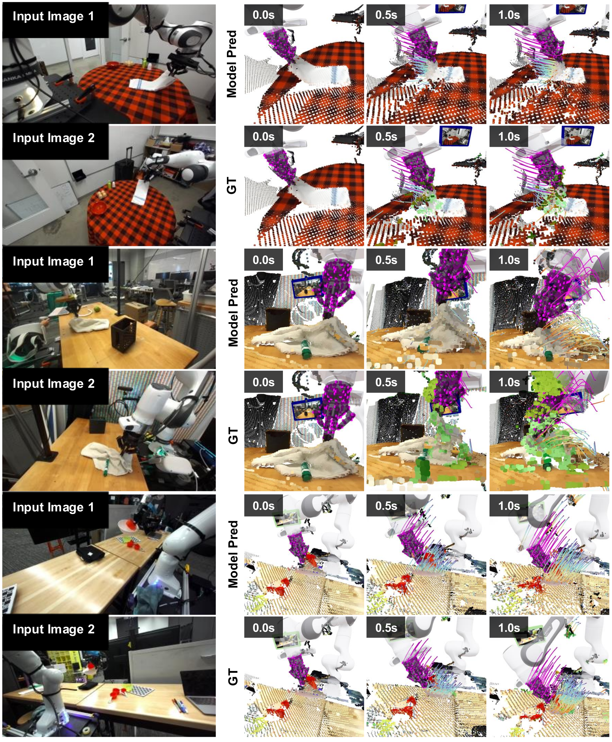
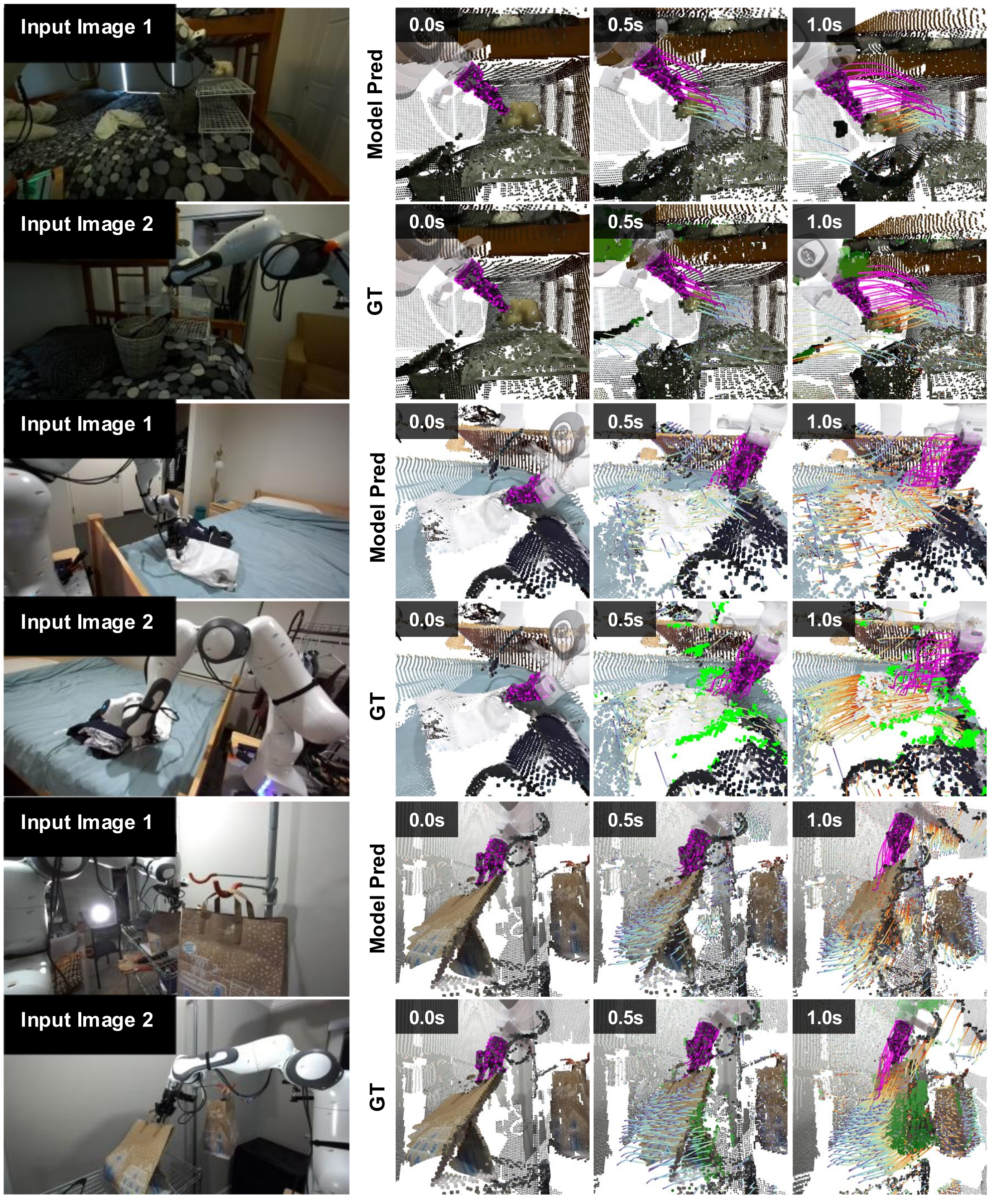
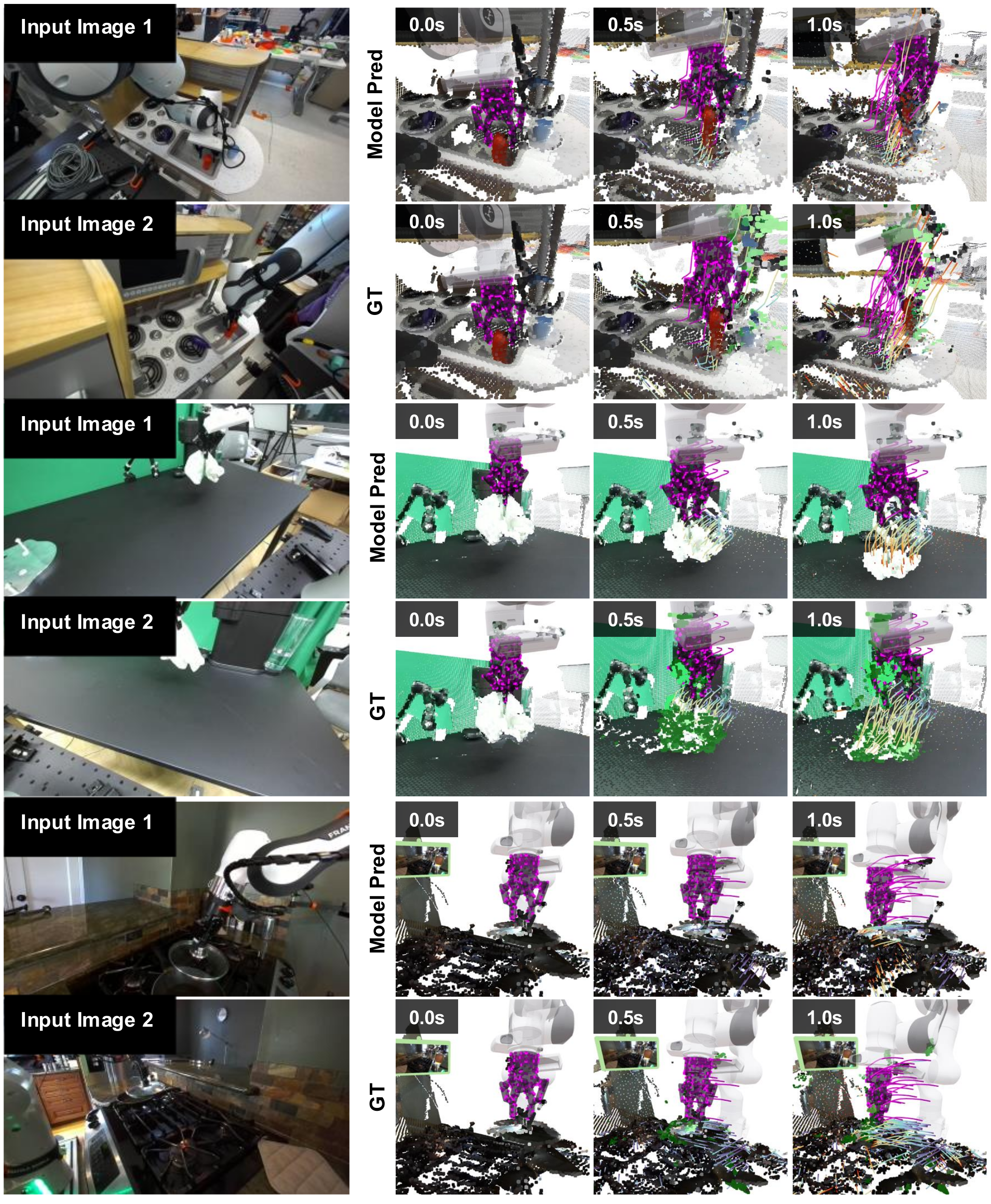
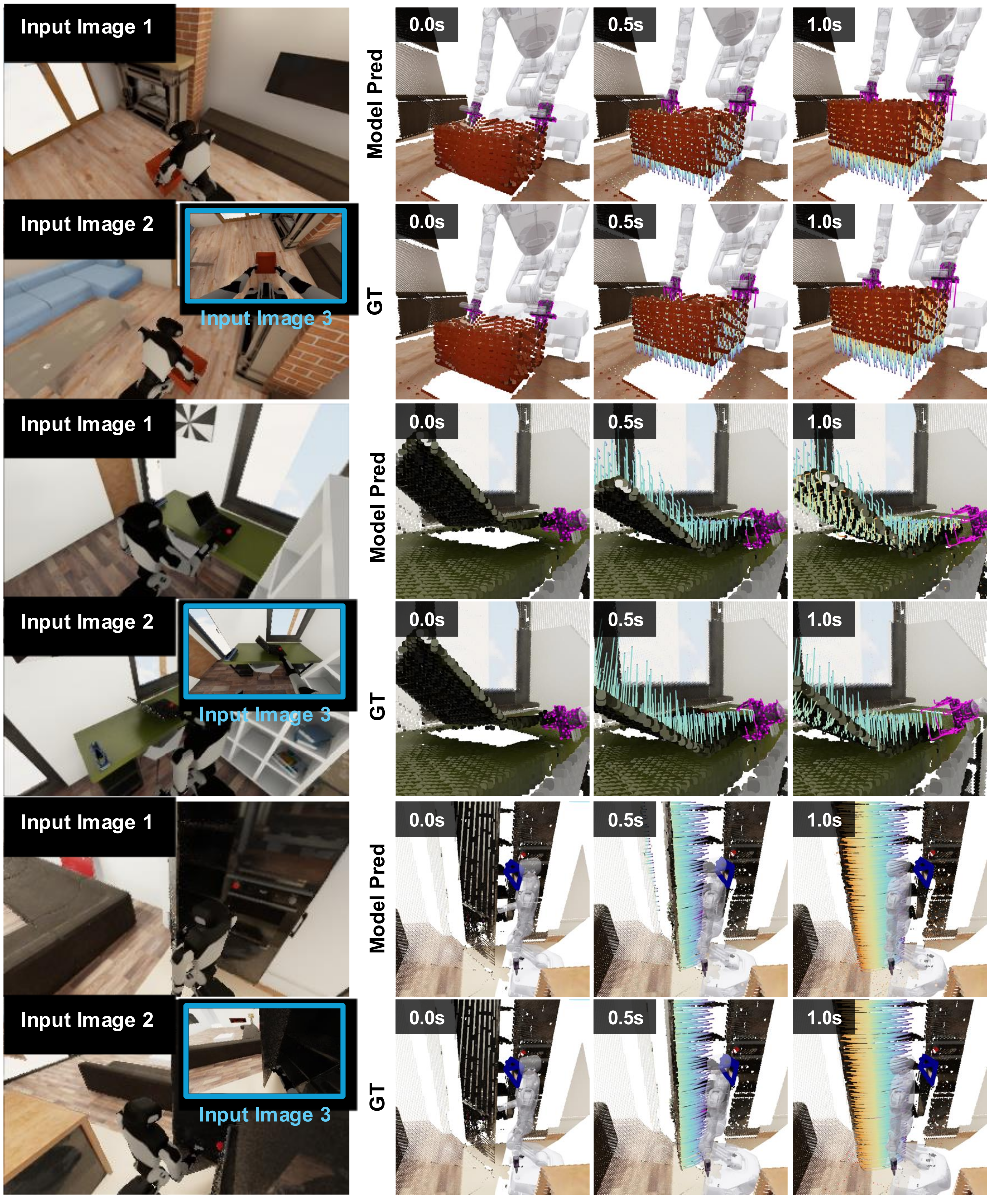
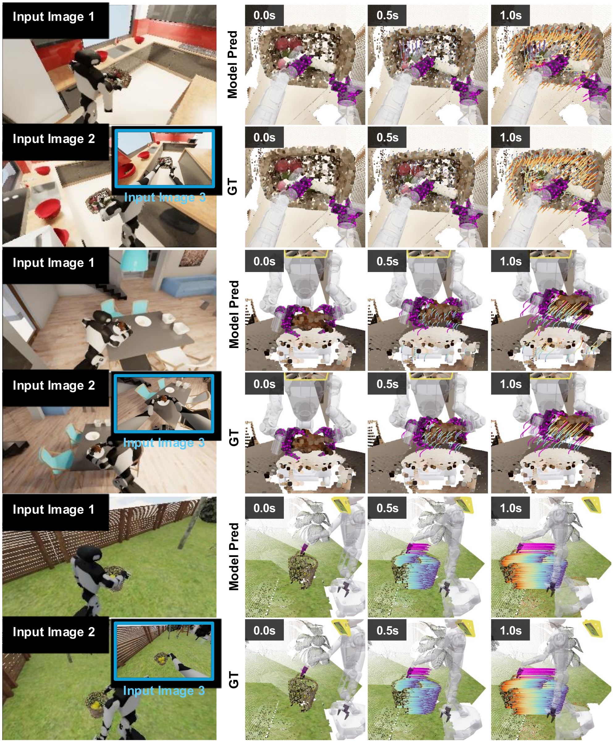
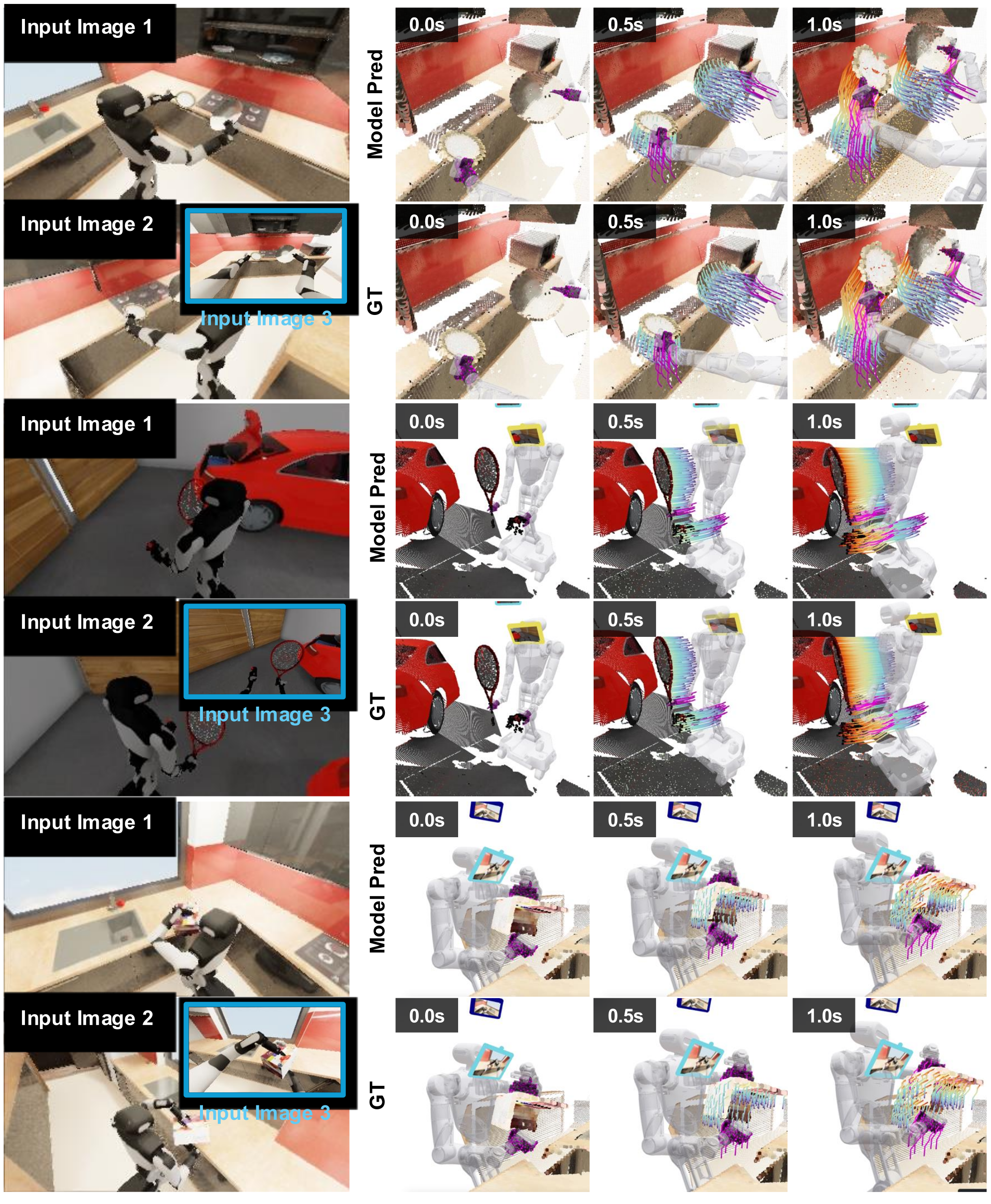
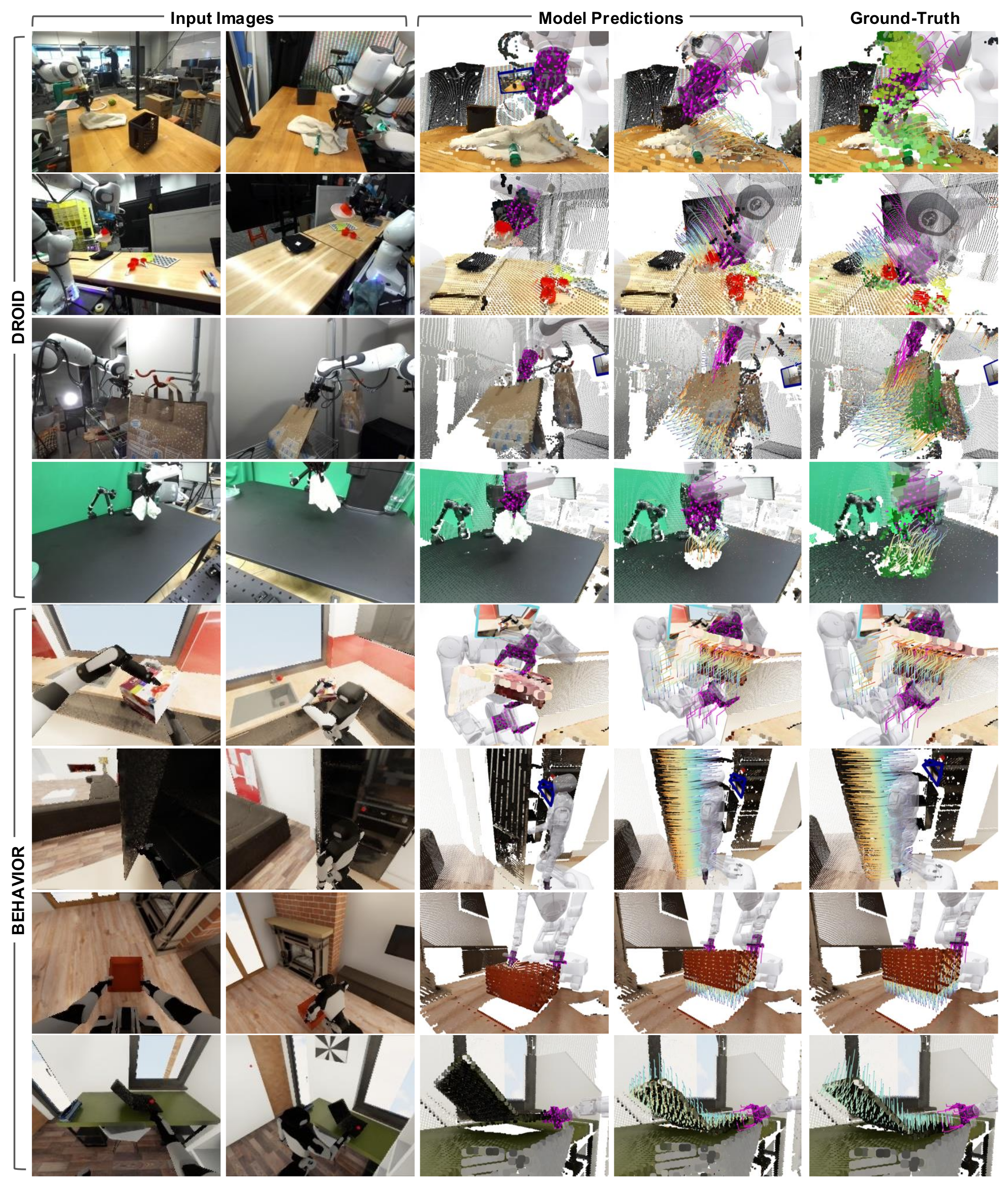
Figures 16–21 retain eighteen complete unseen rollout examples with inputs, predictions and ground-truth frames. They cover cloth, grasping, gravity, glass, bimanual lifting, articulation, baskets and whole-body interaction. Green ground-truth points mark occlusion-related tracking gaps; nearest-neighbor upsampling improves display clarity without adding model spatial resolution. Selected visual examples complement, rather than replace, the filtered quantitative evaluation.