Literature
Display
← All papers

mHC: Manifold-Constrained Hyper-Connections

Zhenda Xie · Yixuan Wei · Huanqi Cao · Chenggang Zhao · Chengqi Deng · Jiashi Li · Damai Dai · Huazuo Gao · Jiang Chang · Kuai Yu · Liang Zhao · Shangyan Zhou · Zhean Xu · Zhengyan Zhang · Wangding Zeng · Shengding Hu · Yuqing Wang · Jingyang Yuan · Lean Wang · Wenfeng Liang

Conference began · ICML 2026 · PMLR 306 ↗

Language models7 min text · CondensedOriginal paper ↗
Contents

Overview

This edition covers arXiv v2, including the full kernel, communication and model-configuration details. Figure 1 compares ordinary residual connections, Hyper-Connections and mHC. The later ICML 2026 publication lists Mingyu Xu where this source version lists Jiang Chang; this edition preserves the v2 byline.
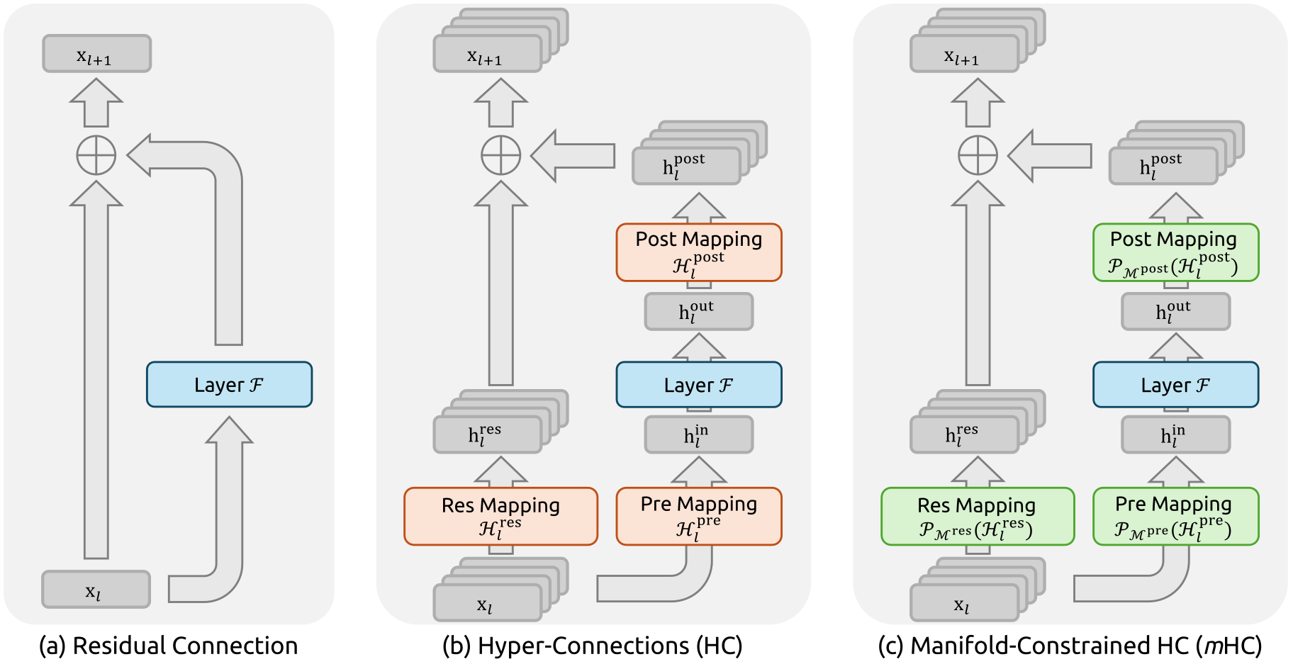
Complete original Figure 1 : Illustrations of Residual Connection Paradigms. This figure compares the structural design of (a) standard Residual Connection, (b) Hyper-Connections (HC), and (c) our proposed Manifold-Constrained Hyper-Connections ( m HC ). Unlike the unconstrained HC, m HC focuses on optimizing the residual connection space by projecting the matrices onto a constrained manifold to ensure stability.
Figure 1: Illustrations of Residual Connection Paradigms. This figure compares the structural design of (a) standard Residual Connection, (b) Hyper-Connections (HC), and (c) our proposed Manifold-Constrained Hyper-Connections (mHC). Unlike the unconstrained HC, mHC focuses on optimizing the residual connection space by projecting the matrices onto a constrained manifold to ensure stability.

At a glance

Intuition. Multiple residual streams are parallel paths carrying intermediate activations. Their mixer acts like a small signal-routing circuit. Repeating a mixer with gain two would amplify a signal exponentially across layers, so the paper restricts how streams can be mixed.

Reading the math. A two-stream example is [[0.8, 0.2], [0.2, 0.8]]: each output is a weighted average, and both row and column totals are one. These constraints define the doubly stochastic mixing matrices; Sinkhorn iterations approximately enforce them. They prevent the mixer from increasing the Euclidean norm across streams, but can still shrink differences. The restriction concerns this mixing operation, not a guarantee that every part of the network preserves signal size.

Hyper-Connections widen a network’s residual stream and learn how its parallel streams mix, but unconstrained repeated mixing can destabilize training and increase memory traffic. mHC approximately constrains residual mixing to nonnegative matrices with unit row and column sums, using Sinkhorn–Knopp normalization. Fused kernels, selective recomputation and communication overlap make the added streams more practical. Experiments on mixture-of-experts language models show better training stability and downstream results, with a reported 6.7% training-time overhead for the optimized four-stream implementation.

1 Introduction

Identity residual paths let information pass directly through depth. Hyper-Connections instead maintain n streams: a pre-map reads them into one layer input, a post-map writes the layer output back, and a residual map mixes the streams. Products of unconstrained residual maps can amplify or suppress signals. mHC targets this mixing with an approximately doubly stochastic constraint, while separately reducing the resulting memory and communication costs. Conserving a stream mean is weaker than reproducing an exact identity map on every feature.

Equations 1–4
𝐱l+1=𝐱l+ℱ⁡(𝐱l,𝒲l),\mathbf{x}_{l+1}=\mathbf{x}_{l}+\mathcal{F}(\mathbf{x}_{l},\mathcal{W}_{l}), (1)
𝐱L=𝐱l+∑i=lL−1ℱ⁡(𝐱i,𝒲i),\mathbf{x}_{L}=\mathbf{x}_{l}+\sum_{i=l}^{L-1}\mathcal{F}(\mathbf{x}_{i},\mathcal{W}_{i}), (2)
𝐱l+1=ℋlres​𝐱l+ℋlpost⊤​ℱ​(ℋlpre​𝐱l,𝒲l),\mathbf{x}_{l+1}=\mathcal{H}_{l}^{\mathrm{res}}\mathbf{x}_{l}+\mathcal{H}_{l}^{\mathrm{post}\,\top}\mathcal{F}(\mathcal{H}_{l}^{\mathrm{pre}}\mathbf{x}_{l},\mathcal{W}_{l}), (3)
𝐱L=(∏i=1L−lℋL−ires)​𝐱l+∑i=lL−1(∏j=1L−1−iℋL−jres)​ℋipost⊤​ℱ​(ℋipre​𝐱i,𝒲i),\mathbf{x}_{L}=\left(\prod_{i=1}^{L-l}\mathcal{H}_{L-i}^{\mathrm{res}}\right)\mathbf{x}_{l}+\sum_{i=l}^{L-1}\left(\prod_{j=1}^{L-1-i}\mathcal{H}_{L-j}^{\mathrm{res}}\right)\mathcal{H}_{i}^{\mathrm{post}\,\top}\mathcal{F}(\mathcal{H}_{i}^{\mathrm{pre}}\mathbf{x}_{i},\mathcal{W}_{i}), (4)

2 Related Works

The paper separates changes inside computational blocks from changes to the topology connecting those blocks. mHC addresses the latter.

2.1 Micro Design

Micro-design includes convolution, attention and feed-forward layers, along with efficiency variants such as grouped-query or latent attention and sparse mixture-of-experts feed-forward computation. These change how each block transforms its inputs.

2.2 Macro Design

Macro-design controls routing and merging across layers. DenseNet, FractalNet and aggregation methods expand paths; recent methods widen or dynamically combine residual states. mHC builds specifically on HC, retaining learned inter-stream communication while constraining the residual map and optimizing its implementation.

3 Preliminary

Represent the widened hidden state as an n×C matrix. Input-dependent projections plus static biases generate the pre-, post- and residual maps; small learned gates modulate the dynamic components. The expensive layer function still receives width C, so residual-state capacity can grow without proportionally enlarging that function’s FLOPs. In Table 1’s ablation, enabling residual mixing gives most of the observed loss improvement (−.022), with pre/post maps reaching −.025/−.027. Disabled maps use specified fixed weights to keep dimensions compatible.

Equation 5
{𝐱~l=RMSNorm​(𝐱l)ℋlpre=αlpre⋅tanh⁡(θlpre​𝐱~l⊤)+𝐛lpreℋlpost=αlpost⋅tanh⁡(θlpost​𝐱~l⊤)+𝐛lpostℋlres=αlres⋅tanh⁡(θlres​𝐱~l⊤)+𝐛lres,\begin{cases}\tilde{\mathbf{x}}_{l}=\text{RMSNorm}(\mathbf{x}_{l})\\ \mathcal{H}^{\mathrm{pre}}_{l}=\alpha_{l}^{\mathrm{pre}}\cdot\tanh(\theta^{\mathrm{pre}}_{l}\tilde{\mathbf{x}}^{\top}_{l})+\mathbf{b}_{l}^{\mathrm{pre}}\\ \mathcal{H}^{\mathrm{post}}_{l}=\alpha_{l}^{\mathrm{post}}\cdot\tanh(\theta^{\mathrm{post}}_{l}\tilde{\mathbf{x}}^{\top}_{l})+\mathbf{b}_{l}^{\mathrm{post}}\\ \mathcal{H}^{\mathrm{res}}_{l}=\alpha_{l}^{\mathrm{res}}\cdot\tanh(\theta^{\mathrm{res}}_{l}\tilde{\mathbf{x}}^{\top}_{l})+\mathbf{b}_{l}^{\mathrm{res}},\\ \end{cases} (5)
Table 1: Ablation Study of HC Components. When a specific mapping (ℋlpre\mathcal{H}^{\mathrm{pre}}_{l}, ℋlpost\mathcal{H}^{\mathrm{post}}_{l}, or ℋlres\mathcal{H}^{\mathrm{res}}_{l}) is disabled, we employ a fixed mapping to maintain dimensional consistency: uniform weights of 1/n1/n for ℋlpre\mathcal{H}^{\mathrm{pre}}_{l}, uniform weights of ones for ℋlpost\mathcal{H}^{\mathrm{post}}_{l}, and the identity matrix for ℋlres\mathcal{H}^{\mathrm{res}}_{l}.
ℋlres\mathcal{H}^{\mathrm{res}}_{l} ℋlpre\mathcal{H}^{\mathrm{pre}}_{l} ℋlpost\mathcal{H}^{\mathrm{post}}_{l} Absolute Loss Gap
0.0\phantom{-\ }0.0\phantom{00}
✓ − 0.022-\ 0.022
✓ ✓ − 0.025-\ 0.025
✓ ✓ ✓ − 0.027-\ 0.027

3.1 Numerical Instability

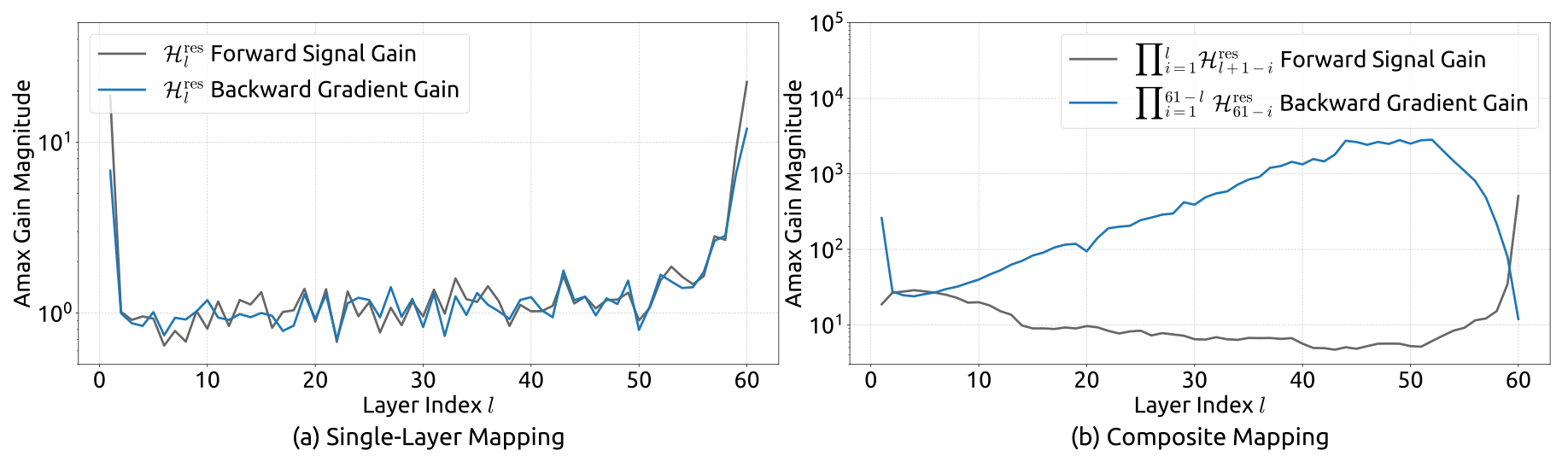
The product of learned residual matrices controls the direct multi-layer signal path. In the 27B HC run, a loss surge near step 12,000 coincides with unstable gradient norms. The reported forward/backward gain diagnostics use row/column sums of the composed map; peaks approach 3,000. These diagnose the residual branch’s propagation, rather than the complete input-dependent network Jacobian.
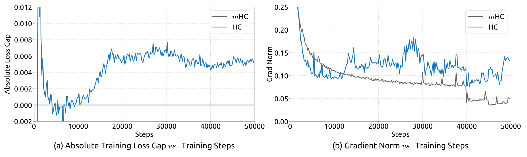
Complete original Figure 2 : Training Instability of Hyper-Connections (HC). This figure illustrates (a) the absolute loss gap of HC relative to m HC, and (b) the comparisons of gradient norms. All results are based on 27B models.
Figure 2: Training Instability of Hyper-Connections (HC). This figure illustrates (a) the absolute loss gap of HC relative to mHC, and (b) the comparisons of gradient norms. All results are based on 27B models.
Complete original Figure 3 : Propagation Instability of Hyper-Connections (HC). This figure illustrates the propagation dynamics of (a) the single-layer mapping ℋ l res \mathcal{H}^{\mathrm{res}}_{l} and (b) the composite mapping ∏ i = 1 L − l ℋ L − i res \prod_{i=1}^{L-l}\mathcal{H}_{L-i}^{\mathrm{res}} within the 27B model. The layer index l l (x-axis) unrolls each standard Transformer block into two independent layers (Attention and FFN). The Amax Gain Magnitude (y-axis) is calculated as the maximum absolute row sum (for the forward signal) and column sum (for the backward gradient), averaged over all tokens in a selected sequence.
Figure 3: Propagation Instability of Hyper-Connections (HC). This figure illustrates the propagation dynamics of (a) the single-layer mapping ℋlres\mathcal{H}^{\mathrm{res}}_{l} and (b) the composite mapping ∏i=1L−lℋL−ires\prod_{i=1}^{L-l}\mathcal{H}_{L-i}^{\mathrm{res}} within the 27B model. The layer index ll (x-axis) unrolls each standard Transformer block into two independent layers (Attention and FFN). The Amax Gain Magnitude (y-axis) is calculated as the maximum absolute row sum (for the forward signal) and column sum (for the backward gradient), averaged over all tokens in a selected sequence.

3.2 System Overhead

Small added FLOP counts can conceal substantial memory traffic. Table 2 counts forward residual-maintenance reads/writes, excluding the layer function itself. Widening also increases saved activations and pipeline communication by roughly the stream expansion factor. Fused kernels, recomputation and scheduling are therefore central to the practical method.

Table 2: Comparison of Memory Access Costs Per Token. This analysis accounts for the overhead introduced by the residual stream maintenance in the forward pass, excluding the internal I/O of the layer function ℱ\mathcal{F}.
Method Operation Read (Elements) Write (Elements)
Residual
Connection
Residual Merge 2​C2C CC
Total I/O 𝟐​𝐂\mathbf{2C} 𝐂\mathbf{C}
Hyper-
Connections
Calculate ℋlpre\mathcal{H}^{\mathrm{pre}}_{l}, ℋlpost\mathcal{H}^{\mathrm{post}}_{l}, ℋlres\mathcal{H}^{\mathrm{res}}_{l} n​CnC n2+2​nn^{2}+2n
ℋlpre\mathcal{H}^{\mathrm{pre}}_{l} n​C+nnC+n CC
ℋlpost\mathcal{H}^{\mathrm{post}}_{l} C+nC+n n​CnC
ℋlres\mathcal{H}^{\mathrm{res}}_{l} n​C+n2nC+n^{2} n​CnC
Residual Merge 2​n​C2nC n​CnC
Total I/O (𝟓​𝐧+𝟏)​𝐂+𝐧𝟐+𝟐​𝐧\mathbf{(5n+1)C+n^{2}+2n} (𝟑​𝐧+𝟏)​𝐂+𝐧𝟐+𝟐​𝐧\mathbf{(3n+1)C+n^{2}+2n}

4 Method

mHC couples constrained mixing with a different coefficient parameterization and an implementation designed for the widened residual state.

4.1 Manifold-Constrained Hyper-Connections

Constrain the residual matrix to the Birkhoff polytope: nonnegative entries and row/column sums equal to one. Such a map forms convex combinations of streams, preserves their mean, is non-expansive in spectral norm, and remains doubly stochastic under composition. It can still contract differences between streams, so the source’s “norm preservation” wording should not be read as preserving every vector’s norm or excluding all vanishing-gradient mechanisms. At n=1 it reduces to the ordinary identity residual map. Pre/post coefficients are separately constrained to be nonnegative.

Equation 6
𝒫ℳres(ℋlres):-{ℋlres∈ℝn×n∣ℋlres𝟏n=𝟏n, 1n⊤ℋlres=𝟏n⊤,ℋlres⩾0},\mathcal{P}_{\mathcal{M}^{\mathrm{res}}}(\mathcal{H}^{\mathrm{res}}_{l})\coloneq\left\{\mathcal{H}^{\mathrm{res}}_{l}\in\mathbb{R}^{n\times n}\mid\mathcal{H}^{\mathrm{res}}_{l}\mathbf{1}_{n}=\mathbf{1}_{n},\ \mathbf{1}^{\top}_{n}\mathcal{H}^{\mathrm{res}}_{l}=\mathbf{1}^{\top}_{n},\ \mathcal{H}^{\mathrm{res}}_{l}\geqslant 0\right\}, (6)

4.2 Parameterization and Manifold Projection

Flatten the entire n×C state before RMS normalization and dynamic projections, allowing each coefficient to depend on all streams. Apply sigmoid to pre-coefficients, twice sigmoid to post-coefficients, and exponentiation followed by alternating column/row normalization to the residual matrix. Sinkhorn–Knopp converges to double stochasticity in the limit; the experiments use twenty iterations, producing an approximation rather than exact unit sums.

Equations 7–9
{𝐱→l′=RMSNorm​(𝐱→l)ℋ~lpre=αlpre⋅(𝐱→l′​φlpre)+𝐛lpreℋ~lpost=αlpost⋅(𝐱→l′​φlpost)+𝐛lpostℋ~lres=αlres⋅mat​(𝐱→l′​φlres)+𝐛lres,\begin{cases}\vec{\mathbf{x}}^{\prime}_{l}=\text{RMSNorm}(\vec{\mathbf{x}}_{l})\\ \tilde{\mathcal{H}}^{\mathrm{pre}}_{l}=\alpha_{l}^{\mathrm{pre}}\cdot(\vec{\mathbf{x}}^{\prime}_{l}\varphi^{\mathrm{pre}}_{l})+\mathbf{b}_{l}^{\mathrm{pre}}\\ \tilde{\mathcal{H}}^{\mathrm{post}}_{l}=\alpha_{l}^{\mathrm{post}}\cdot(\vec{\mathbf{x}}^{\prime}_{l}\varphi^{\mathrm{post}}_{l})+\mathbf{b}_{l}^{\mathrm{post}}\\ \tilde{\mathcal{H}}^{\mathrm{res}}_{l}=\alpha_{l}^{\mathrm{res}}\cdot\text{mat}(\vec{\mathbf{x}}^{\prime}_{l}\varphi^{\mathrm{res}}_{l})+\mathbf{b}_{l}^{\mathrm{res}},\\ \end{cases} (7)
{ℋlpre=σ⁡(ℋ~lpre)ℋlpost=2​σ​(ℋ~lpost)ℋlres=Sinkhorn-Knopp​(ℋ~lres),\begin{cases}\mathcal{H}^{\mathrm{pre}}_{l}=\sigma(\tilde{\mathcal{H}}^{\mathrm{pre}}_{l})\\ \mathcal{H}^{\mathrm{post}}_{l}=2\sigma(\tilde{\mathcal{H}}^{\mathrm{post}}_{l})\\ \mathcal{H}^{\mathrm{res}}_{l}=\text{Sinkhorn-Knopp}(\tilde{\mathcal{H}}^{\mathrm{res}}_{l}),\end{cases} (8)
𝐌(t)=𝒯r​(𝒯c​(𝐌(t−1))),\mathbf{M}^{(t)}=\mathcal{T}_{r}\left(\mathcal{T}_{c}(\mathbf{M}^{(t-1)})\right), (9)

4.3 Efficient Infrastructure Design

The optimized n=4 implementation reports 6.7% additional training time. This is an infrastructure-dependent measurement, not a cost-free architectural change.

4.3.1 Kernel Fusion

Move RMS division after projection and absorb normalization weights into the projection. Fuse the projection and norm scans; fuse small coefficient operations; run Sinkhorn iterations in one kernel with a custom recomputing backward pass. Additional kernels apply the pre-map and combine post-map, residual mixing and merge. For the latter kernel, reads fall from (3n+1)C to (n+1)C and writes from 3nC to nC. Equations 10–19 retain the precise tensor shapes, precision choices and transformations. Most kernels use TileLang.

Equations 10–19
φl\displaystyle\varphi_{l} :tfloat32\displaystyle:\text{tfloat32} [n​C,n2+2​n]\displaystyle[nC,n^{2}+2n] (10)
𝐱→l\displaystyle\vec{\mathbf{x}}_{l} :bfloat16\displaystyle:\text{bfloat16} [1,n​C]\displaystyle[1,nC] (11)
αlpre,αlpost,αlres\displaystyle\alpha_{l}^{\mathrm{pre}},\alpha_{l}^{\mathrm{post}},\alpha_{l}^{\mathrm{res}} :float32\displaystyle:\text{float32} Scalars (12)
𝐛l\displaystyle\mathbf{b}_{l} :float32\displaystyle:\text{float32} [1,n2+2​n]\displaystyle[1,n^{2}+2n] (13)
[ℋ~~lpre,ℋ~~lpost,ℋ~~lres]\displaystyle\left[{\tilde{\tilde{\mathcal{H}}}^{\mathrm{pre}}_{l}},{\tilde{\tilde{\mathcal{H}}}^{\mathrm{post}}_{l}},{\tilde{\tilde{\mathcal{H}}}^{\mathrm{res}}_{l}}\right] :float32\displaystyle:\text{float32} =𝐱→l​φl\displaystyle=\vec{\mathbf{x}}_{l}\varphi_{l} (14)
r\displaystyle r :float32\displaystyle:\text{float32} =‖𝐱→l‖2/n​C\displaystyle=\left\|\vec{\mathbf{x}}_{l}\right\|_{2}/\sqrt{nC} (15)
[ℋ~lpre,ℋ~lpost,ℋ~lres]\displaystyle\left[\tilde{\mathcal{H}}^{\mathrm{pre}}_{l},\tilde{\mathcal{H}}^{\mathrm{post}}_{l},\tilde{\mathcal{H}}^{\mathrm{res}}_{l}\right] :float32\displaystyle:\text{float32} =1/r⁡[αlpre​ℋ~~lpre,αlpost​ℋ~~lpost,αlres​ℋ~~lres]+𝐛l\displaystyle=1/r\left[\alpha_{l}^{\mathrm{pre}}{\tilde{\tilde{\mathcal{H}}}^{\mathrm{pre}}_{l}},\alpha_{l}^{\mathrm{post}}{\tilde{\tilde{\mathcal{H}}}^{\mathrm{post}}_{l}},\alpha_{l}^{\mathrm{res}}{\tilde{\tilde{\mathcal{H}}}^{\mathrm{res}}_{l}}\right]+\mathbf{b}_{l} (16)
ℋlpre\displaystyle\mathcal{H}^{\mathrm{pre}}_{l} :float32\displaystyle:\text{float32} =σ⁡(ℋ~lpre)\displaystyle=\sigma\left(\tilde{\mathcal{H}}^{\mathrm{pre}}_{l}\right) (17)
ℋlpost\displaystyle\mathcal{H}^{\mathrm{post}}_{l} :float32\displaystyle:\text{float32} =2​σ​(ℋ~lpost)\displaystyle=2\sigma\left(\tilde{\mathcal{H}}^{\mathrm{post}}_{l}\right) (18)
ℋlres\displaystyle\mathcal{H}^{\mathrm{res}}_{l} :float32\displaystyle:\text{float32} =Sinkhorn-Knopp​(ℋ~lres)\displaystyle=\text{Sinkhorn-Knopp}\left(\tilde{\mathcal{H}}^{\mathrm{res}}_{l}\right) (19)

4.3.2 Recomputing

Discard mHC intermediates after the forward pass and recompute them in blocks during backward, without rerunning the expensive layer function. Save the block’s input plus each layer-function output. Balancing resident block inputs against transient reconstructed states gives the approximate block length √(nL/(n+2)) in Equation 20. Blocks cannot cross pipeline stages; the implementation aligns their boundaries with stages. Table 3 preserves which activations are stored or transient.

Table 3: Stored and Recomputed Intermediate Activations We list per token activation preserved for the backward pass and the transient activation recomputed in LrL_{r} consecutive layers. Layer l0l_{0} represents the first layer in LrL_{r} layers and layer ll is in [l0,l0+Lr−1][l_{0},l_{0}+L_{r}-1].
Activations 𝐱l0\mathbf{x}_{l_{0}} ℱ⁡(ℋlpre​𝐱l,𝒲l)\mathcal{F}(\mathcal{H}^{\mathrm{pre}}_{l}\mathbf{x}_{l},\mathcal{W}_{l}) 𝐱l\mathbf{x}_{l} ℋlpre​𝐱l\mathcal{H}^{\mathrm{pre}}_{l}\mathbf{x}_{l} RMSNorm​(ℋlpre​𝐱l)\text{RMSNorm}(\mathcal{H}^{\mathrm{pre}}_{l}\mathbf{x}_{l})
Size (Elements) n​CnC CC n​CnC CC CC
Stored Method Every LrL_{r} layers Every layer Transient inside LrL_{r} layers
Equation 20
Lr∗=arg⁡minLr⁡[n​C×⌈LLr⌉+(n+2)​C×Lr]≈n​Ln+2.L_{r}^{*}=\arg\min_{L_{r}}\left[nC\times\left\lceil\frac{L}{L_{r}}\right\rceil+(n+2)C\times L_{r}\right]\approx\sqrt{\frac{nL}{n+2}}. (20)

4.3.3 Overlapping Communication in DualPipe

Extend DualPipe to overlap the additional communication and block recomputation. Run the feed-forward post/residual kernel on a high-priority compute stream and avoid long-running persistent attention kernels that would delay it. Cached stage-input activations let recomputation proceed independently of incoming pipeline communication. Figure 4 is a scheduling schematic; block widths do not represent measured durations.

Complete original Figure 4 : Communication-Computation Overlapping for m HC. We extend the DualPipe schedule to handle the overhead introduced by m HC. Lengths of each block are illustrative only and do not represent actual duration. (F), (B), (W) refers to forward pass, backward pass, weight gradient computation, respectively. ℱ A ​ and ​ ℱ M \mathcal{F}^{\mathrm{A}}\ \text{and}\ \mathcal{F}^{\mathrm{M}} represents kernels corresponded to Attention and MLP, respectively.
Figure 4: Communication-Computation Overlapping for mHC. We extend the DualPipe schedule to handle the overhead introduced by mHC. Lengths of each block are illustrative only and do not represent actual duration. (F), (B), (W) refers to forward pass, backward pass, weight gradient computation, respectively. ℱA​and​ℱM\mathcal{F}^{\mathrm{A}}\ \text{and}\ \mathcal{F}^{\mathrm{M}} represents kernels corresponded to Attention and MLP, respectively.

5 Experiments

Experiments compare ordinary residual connections, unconstrained HC and mHC using the same four-stream expansion for the latter two.

5.1 Experimental Setup

DeepSeek-V3-inspired mixture-of-experts models cover 3B, 9B and 27B total parameters, with parameter-proportional training data. A separate 3B run examines token scaling on approximately one trillion tokens. The principal stability and downstream comparison uses the 27B model; Appendix A gives all active-parameter counts and schedules.

5.2 Main Results

The 27B mHC run finishes .021 loss below the baseline and avoids HC’s reported loss/gradient disturbance. It beats the baseline on all eight displayed benchmarks and HC on seven; MATH is 26.0 for mHC versus 26.4 for HC. Relative to HC, BBH rises 2.1 points and DROP 2.3 points. Table 4 preserves task-specific metrics and zero/few-shot settings, so these gains are percentage-point score differences rather than a uniform relative improvement.
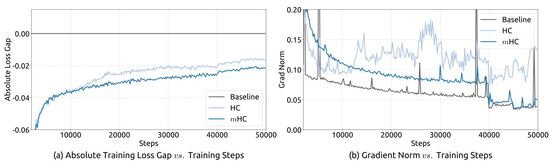
Complete original Figure 5 : Training Stability of Manifold-Constrained Hyper-Connections ( m HC). This figure illustrates (a) the absolute training loss gap of m HC and HC relative to the baseline, and (b) the gradient norm of the three methods. All experiments utilize the 27B model. The results demonstrate that m HC exhibits improved stability in terms of both loss and gradient norm.
Figure 5: Training Stability of Manifold-Constrained Hyper-Connections (mHC). This figure illustrates (a) the absolute training loss gap of mHC and HC relative to the baseline, and (b) the gradient norm of the three methods. All experiments utilize the 27B model. The results demonstrate that mHC exhibits improved stability in terms of both loss and gradient norm.
Table 4: System-level Benchmark Results for 27B Models. This table compares the zero-shot and few-shot performance of the Baseline, HC, and mHC across 8 diverse downstream benchmarks. mHC consistently outperforms the Baseline and surpasses HC on the majority of benchmarks, demonstrating its effectiveness in large-scale pre-training.
Benchmark BBH DROP GSM8K HellaSwag MATH MMLU PIQA TriviaQA
(Metric) (EM) (F1) (EM) (Acc.) (EM) (Acc.) (Acc.) (EM)
# Shots 3-shot 3-shot 8-shot 10-shot 4-shot 5-shot 0-shot 5-shot
27B Baseline 43.8 47.0 46.7 73.7 22.0 59.0 78.5 54.3
27B w/ HC 48.9 51.6 53.2 74.3 26.4 63.0 79.9 56.3
27B w/ mHC 51.0 53.9 53.8 74.7 26.0 63.4 80.5 57.6

5.3 Scaling Experiments

The loss advantage over the baseline persists across the three reported compute/model scales, with some attenuation, and through the separate 3B token-scaling trajectory. Figure 6 provides the absolute gaps and relative ratios. These observations support scaling within the tested configurations; the additional in-house large-scale result is not accompanied by a comparable detailed benchmark table.
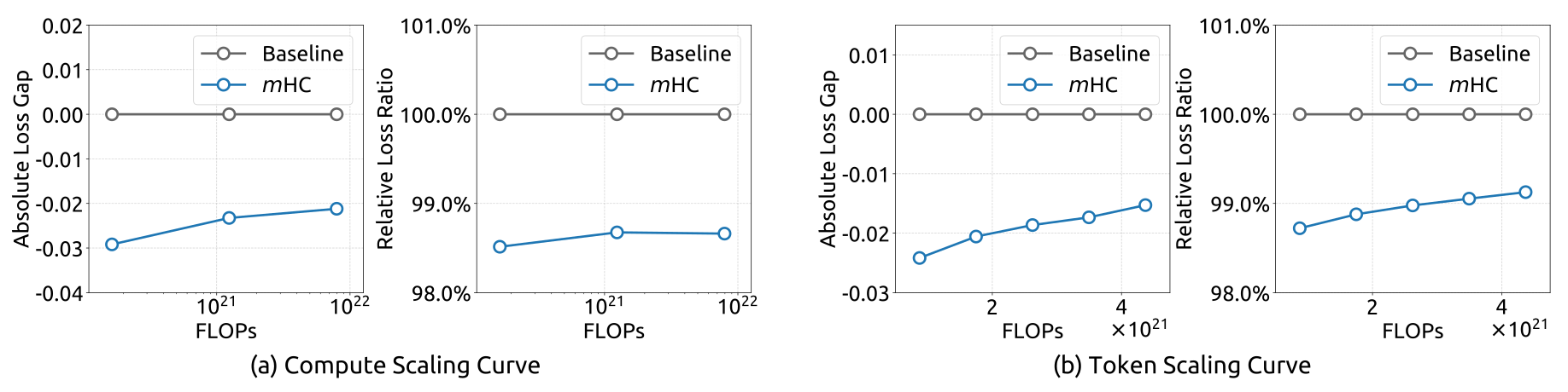
Complete original Figure 6 : Scaling properties of m HC compared to the Baseline. (a) Compute Scaling Curve. Solid lines depict the performance gap across different compute budgets. Each point represents a specific compute-optimal configuration of model size and dataset size, scaling from 3B and 9B to 27B parameters. (b) Token Scaling Curve. Trajectory of the 3B model during training. Each point represents the model’s performance at different training tokens.
Detailed architectures and training configurations are provided in Appendix A.1 .
Figure 6: Scaling properties of mHC compared to the Baseline. (a) Compute Scaling Curve. Solid lines depict the performance gap across different compute budgets. Each point represents a specific compute-optimal configuration of model size and dataset size, scaling from 3B and 9B to 27B parameters. (b) Token Scaling Curve. Trajectory of the 3B model during training. Each point represents the model’s performance at different training tokens. Detailed architectures and training configurations are provided in Appendix A.1.

5.4 Stability Analysis

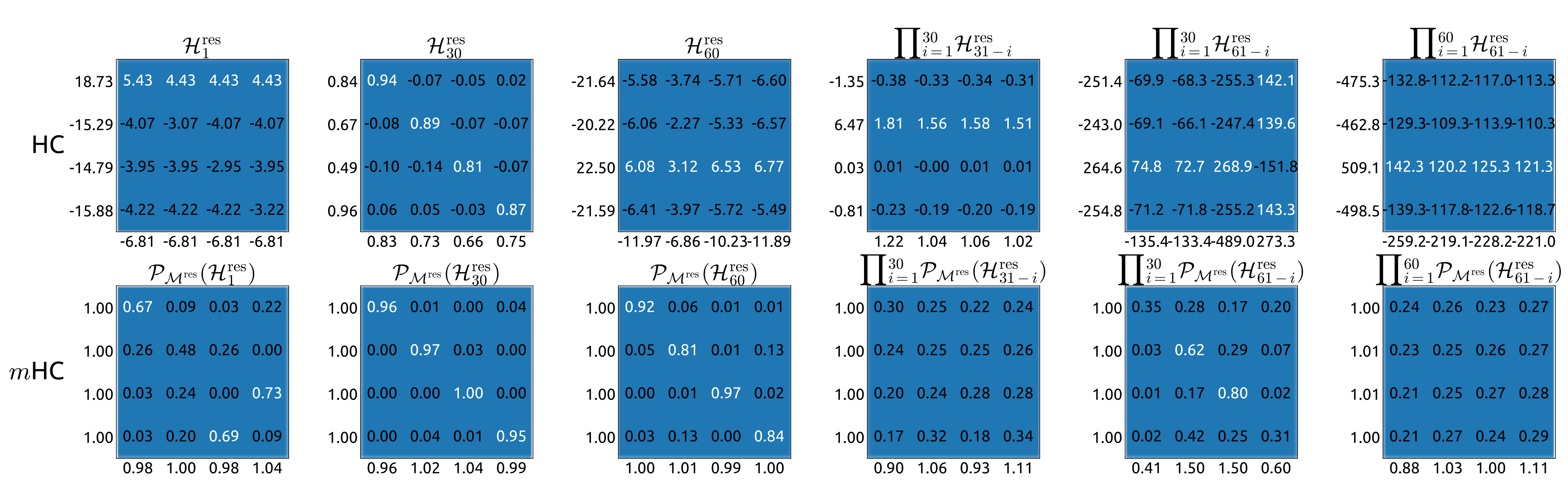
With twenty Sinkhorn iterations, single-layer backward gain deviates slightly from one and the composed-map gain reaches approximately 1.6. This is far below HC’s roughly 3,000 peak, but confirms that the practical constraint is approximate. Figures 7–8 retain all gain curves and representative matrices, averaged over tokens in a selected sequence. They measure the specified residual-map diagnostics rather than proving stability for every input or the full nonlinear network.
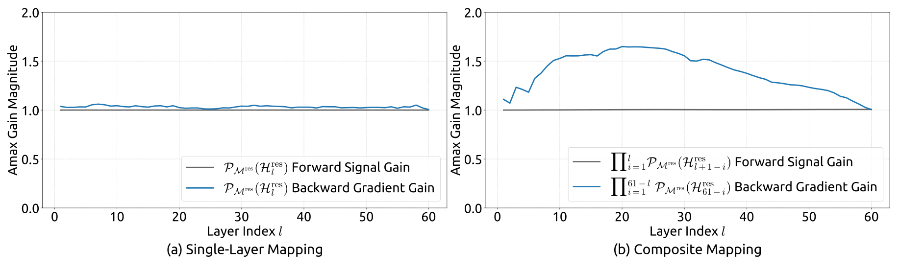
Complete original Figure 7 : Propagation Stability of Manifold-Constrained Hyper-Connections ( m HC). This figure illustrates the propagation dynamics of (a) the single-layer mapping 𝒫 ℳ res ​ ( ℋ l res ) \mathcal{P}_{\mathcal{M}^{\mathrm{res}}}(\mathcal{H}^{\mathrm{res}}_{l}) and (b) the composite mapping ∏ i = 1 L − l 𝒫 ℳ res ​ ( ℋ L − i res ) \prod_{i=1}^{L-l}\mathcal{P}_{\mathcal{M}^{\mathrm{res}}}(\mathcal{H}_{L-i}^{\mathrm{res}}) within the 27B model. The results demonstrate that m HC significantly enhances propagation stability compared to HC.
Figure 7: Propagation Stability of Manifold-Constrained Hyper-Connections (mHC). This figure illustrates the propagation dynamics of (a) the single-layer mapping 𝒫ℳres​(ℋlres)\mathcal{P}_{\mathcal{M}^{\mathrm{res}}}(\mathcal{H}^{\mathrm{res}}_{l}) and (b) the composite mapping ∏i=1L−l𝒫ℳres​(ℋL−ires)\prod_{i=1}^{L-l}\mathcal{P}_{\mathcal{M}^{\mathrm{res}}}(\mathcal{H}_{L-i}^{\mathrm{res}}) within the 27B model. The results demonstrate that mHC significantly enhances propagation stability compared to HC.
Complete original Figure 8 : Visualizations of Learnable Mappings. This figure displays representative single-layer and composite mappings for HC (first row) and m HC (second row). Each matrix is computed by averaging over all tokens within a selected sequence. The labels annotated along the y-axis and x-axis indicate the forward signal gain (row sum) and the backward gradient gain (column sum), respectively.
Figure 8: Visualizations of Learnable Mappings. This figure displays representative single-layer and composite mappings for HC (first row) and mHC (second row). Each matrix is computed by averaging over all tokens within a selected sequence. The labels annotated along the y-axis and x-axis indicate the forward signal gain (row sum) and the backward gradient gain (column sum), respectively.

6 Conclusion and Outlook

Constraining inter-stream mixing and engineering its execution yields a more stable practical form of HC in the reported language-model runs. Mean conservation and non-expansive mixing explain part of the motivation; empirical training behavior supplies the broader evidence. Other geometric constraints and the balance between mixing flexibility and stability remain future work.

Appendix A Appendix

The appendix supplies the complete model, optimizer and training configurations used in the experiments.

A.1 Detailed Model Specifications and Hyper-parameters.

The 3B/9B/27B models have 12/18/30 layers and 612M/1.66B/4.14B active parameters. Proportional-data runs use 39.3B/105B/262B tokens; the separate 3B run uses 1.05T. All use length 4,096, expansion four, initial dynamic gates .01 and twenty Sinkhorn iterations. Table 5 retains expert counts, latent-attention and rotary settings, normalization, batch sizes, steps, warmup and learning-rate schedules. Total parameter count and per-token active parameter count are distinct quantities.

Table 5: Detailed Model Specifications and Hyper-parameters. This table presents the architectural configurations for the 3B, 9B, and 27B models based on the DeepSeek-V3 (Liu et al., 2024b) architecture. It outlines the specific hyper-parameters for mHC and HC, including the residual stream expansion and Sinkhorn-Knopp settings, alongside the optimization and training protocols used in the experiments.
Attribute 3B 9B 27B 3B
1T Tokens
Vocab Params 331M 496M 662M 331M
Active Params 612M 1.66B 4.14B 612M
Total Params 2.97B 9.18B 27.0B 2.97B
Layers 12 18 30 12
Leading Dense Layers 1 1
Routed Experts 64 64 72 64
Active Experts 6 6
Shared Experts 2 2
Dimension 1280 1920 2560 1280
FFN Dimension 896 1280 1536 896
Load Balancing Method Loss-Free (Wang et al., 2024) Loss-Free
Attention Heads 16 24 32 16
Attention Dimension 128 128
Attention Variant MLA (Liu et al., 2024a) MLA
KV Rank 512 512
Position Embedding RoPE (Su et al., 2024) RoPE
RoPE Dimension 64 64
RoPE θ\theta 10000 10000
Layer Norm Type RMSNorm (Zhang and Sennrich, 2019) RMSNorm
Layer Norm ε\varepsilon 1e-20 1e-20
mHC/HC Expansion Rate nn 4 4
mHC/HC Gating Factor Init α\alpha 0.01 0.01
mHC Sinkhorn-Knopp tmaxt_{\text{max}} 20 20
Sequence Length 4096 4096
Vocab Size 129280 129280
Batch Size 320 512 1280 2560
Training Steps 30000 50000 50000 100000
Training Tokens 39.3B 105B 262B 1.05T
Warmup Steps 2000 2000
Optimizer AdamW (Loshchilov and Hutter, 2017) AdamW
AdamW Betas (0.9, 0.95) (0.9, 0.95)
AdamW ε\varepsilon 1e-20 1e-20
Base Learning Rate 8.6e-4 5.9e-4 4.0e-4 9.0e-4
Lr Scheduler Step Step
Lr Decay Step Ratio [0.8 ×\times, 0.9 ×\times] [0.8 ×\times, 0.9 ×\times]
Lr Decay Rate [0.316, 0.1] [0.316, 0.1]
Weight Decay 0.1 0.1
Concept demonstration

Open image ↗