Overview
The work has an open review record at OpenReview. The study compares technical choices within explicit latent world-model planning.
At a glance
Intuition. A world model can imagine convincing future frames and still choose the wrong action: the representation may miss small task-relevant differences, or the planner may get stuck before finding a useful route. This study varies the encoder, predictor, training objective, observation context and planning algorithm within a common family of explicit latent JEPA world models. It then combines favorable choices into stronger task-specific recipes. The key result is practical and conditional: proprioception, short rollout training, suitable image features and the optimizer all matter, while scaling and architecture preferences change with the domain. Results include simulation and offline real-robot action comparisons. They do not prove a universal optimal JEPA architecture or that lower prediction loss necessarily yields higher closed-loop success.
1 Introduction
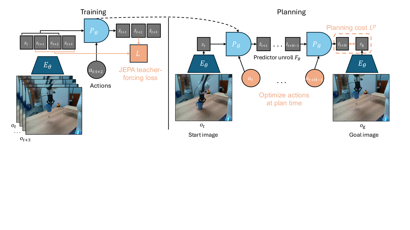
The work studies implementation choices within a specified model family rather than proposing a new general JEPA principle. A frozen visual encoder supplies state features, an action-conditioned predictor learns their dynamics, and a goal-distance planner selects actions. Isolating these components reveals why promising predictive representations can fail as controllers.
2 Related work
World modeling and planning.
World-model planning uses learned dynamics to evaluate candidate futures. The JEPA-WM family here avoids pixel reconstruction and reward training for its main predictive objective. Related generative and policy-learning systems differ in supervision and deployment procedure.
Explicit and implicit world models.
Explicit models generate successive latent states and can be paired with different costs and search methods. Implicit approaches fold temporal information or value-like structure into representations. These are different modeling commitments, not interchangeable implementations of the same rollout.
Goal-conditioned RL.
Goal-conditioned reinforcement learning learns how to reach goals through values, policies or representation distances. Its offline reward-free data can resemble JEPA training data, but amortized policy execution differs from optimizing fresh action sequences through an explicit predictor.
Robotics.
Classical model-predictive control, visual servoing and vision-language-action policies provide complementary robotics context. They differ in dynamics knowledge, task supervision, sensors and whether computation occurs during training or planning.
3 Background
The background formalizes the common training and deployment pipeline. It is the shared experimental framework rather than a new algorithmic contribution.
Training method.
A fixed visual encoder and optional learned proprioceptive encoder produce state embeddings. An action encoder and predictor learn next-state features with teacher forcing. Frozen visual targets avoid co-adaptation collapse but inherit the pretrained encoder’s information and geometry.
Equation 1
| (1) |
Planning.
The planner searches action sequences whose rolled-out final representation matches the encoded goal, with optional proprioceptive weighting. A sliding context window supplies recent predicted states. Goal distance is a heuristic task cost whose usefulness depends on both perception and search.
Equations 2–4
| (2) |
| (3) | ||||
| (4) |
| Component | Candidates | Best: [1pt] Simu. Nav. | Best: [1pt] Real Manip. |
|---|---|---|---|
| Encoder | |||
| Visual encoder | DINOv2 (ViT-S/B/L), DINOv3 (L), V-JEPA (L), V-JEPA-2 (L) | DINOv2-S | DINOv3-L |
| Predictor | |||
| Architecture | Feat. cond. + sincos, Seq. cond. + RoPE, Feat. cond. + RoPE, | AdaLN + RoPE | AdaLN + RoPE |
| AdaLN + RoPE, AdaLN-zero + RoPE | |||
| Depth | 3, 6, 9, 12 | 6 | 12 |
| Training | |||
| Rollout steps | 1-step (teacher forcing), 2-step, 3-step, 6-step | 2 | 6 |
| Context length () | 1, 2, 3, 5, 7, 9, 14 | 3 | 5 |
| Proprioception | With / Without | ✓ | |
| Planning | |||
| Optimizer | CEM, NG (NeverGrad), Adam, GD | CEM | CEM |
| Cost | , | ||
4 Studied design choices
The study first tunes planning choices, then varies training and architecture from a stated baseline, and finally tests scaling and combined recipes. This staged protocol is more informative than assuming a named model’s success follows from its high-level objective alone.
Planner.
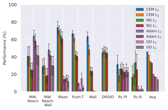
Sampling-based CEM and Nevergrad optimization are compared with gradient descent and Adam through the same predictive cost. Horizons, context, candidate populations and iteration counts control runtime and success. Nevergrad’s meta-optimizer chooses its internal search method from the parameterization and budget.
Multistep rollout training.
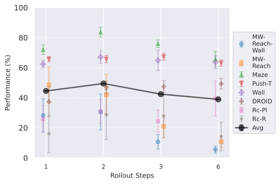
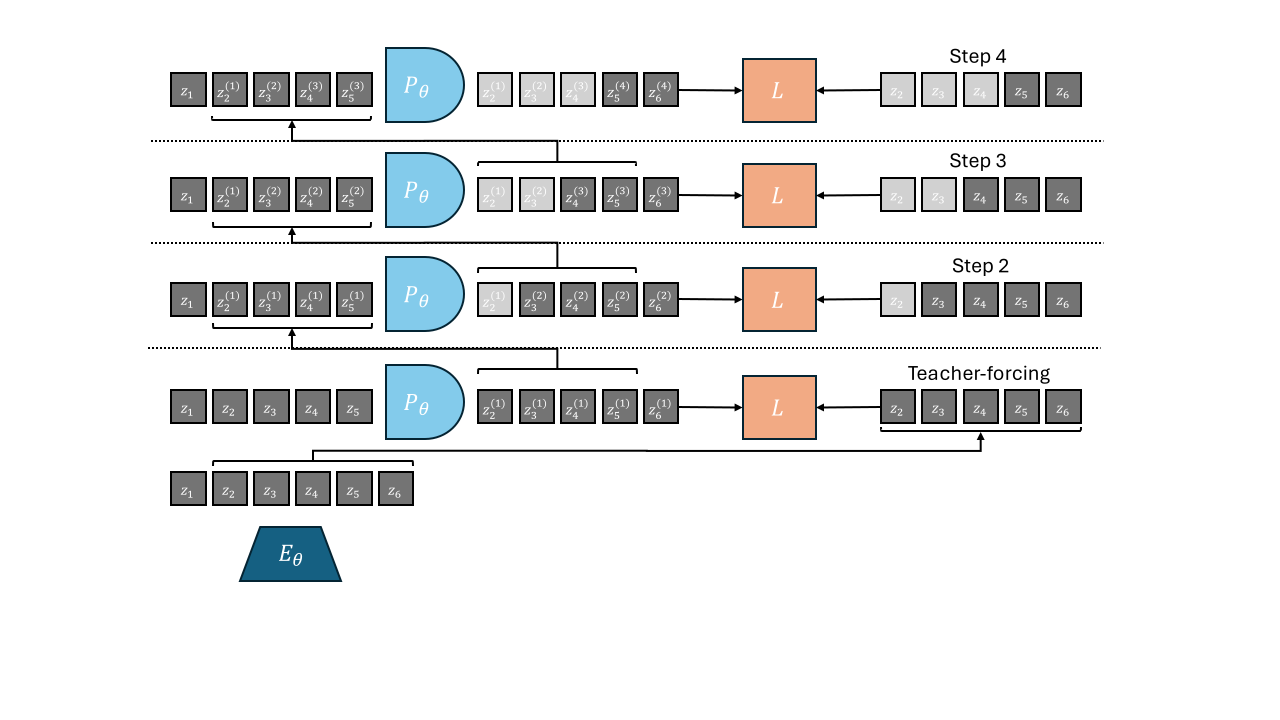
Teacher forcing sees real context, while rollout training also sees the model’s own predicted context. Additional rollout losses aim to reduce the train–deployment mismatch. Truncated derivatives limit backpropagation depth; more rollout steps need not monotonically improve local accuracy or control.
Equation 5
| (5) |
Proprioception.
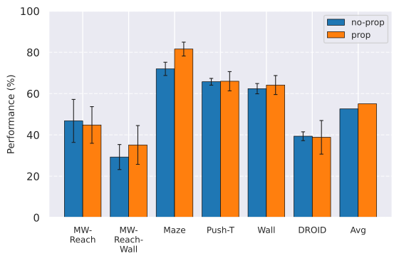
Proprioceptive inputs add precise state measurements to image features. Both visual and proprioceptive predictions are trained where used. A vision-only versus augmented comparison therefore changes the available information, not merely the architecture.
Training context size.
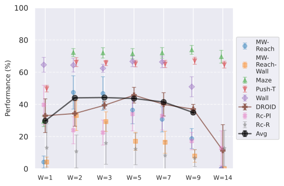
Training context lengths are varied from one to fourteen frames. Longer history can reveal velocity or acceleration, but changes available trajectory slices and prediction difficulty.
Encoder type.
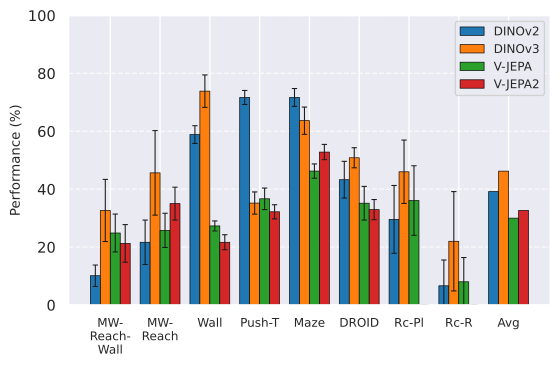
Frozen DINOv2, DINOv3, V-JEPA and V-JEPA2 encoders are compared with token counts and preprocessing controlled as described. Video encoders are applied to duplicated-frame inputs in the selected setting, so this is not an unrestricted comparison of every possible video encoding procedure.
Predictor architecture.
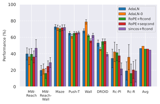
Action information can enter as concatenated features, separate tokens or per-layer adaptive normalization. Positional encoding and zero initialization are also varied. Action-to-visual capacity ratios can confound comparisons, motivating additional matched-ratio controls.
Model and data scaling.
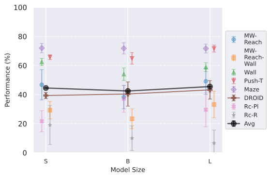
Encoder size, predictor width/depth and data fraction are varied. Larger capacity can help complex real-world data while making optimization harder or providing little benefit on simpler simulations.
5 Experiments
5.1 Evaluation Setup.
Datasets.
The study uses simulated navigation/manipulation datasets and DROID-trained models evaluated on offline Franka videos and RoboCasa transfer. The DROID action score compares planned commands with recorded commands; it is not a measured real-robot task-completion rate.
Goal definition.
Goal states come from expert trajectories, held-out observations or simulator samplers depending on the task. Proprioceptive goal costs are weighted differently where state conventions align, and omitted for the stated cross-domain comparison.
Metrics.
Success is the main control metric, supplemented by latent rollout error, decoded-state error and image reconstruction diagnostics. These supplementary measures inspect model behavior but do not guarantee that a particular optimizer finds a useful action sequence.
Statistical significance.
Final recipes are trained with three seeds and evaluated across multiple episodes and checkpoints. Smoothing across training epochs and sampling multiple task pairs reduces noise but should be distinguished from independent training replications.
5.2 Results
Accurate autoregressive prediction is not sufficient for planning success. The subsequent controls locate failures in objective geometry, observation precision, optimization and domain shift.
Comparing planning optimizers.
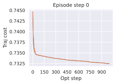
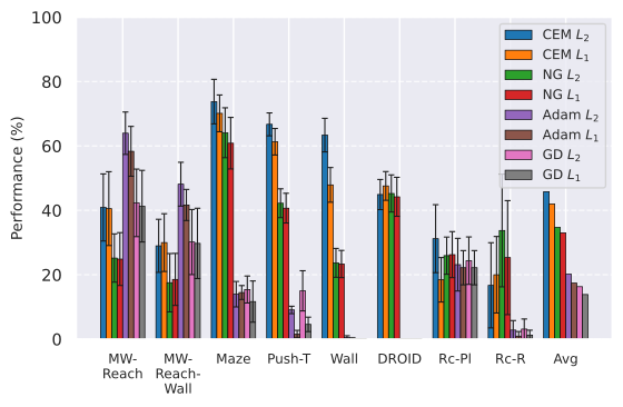
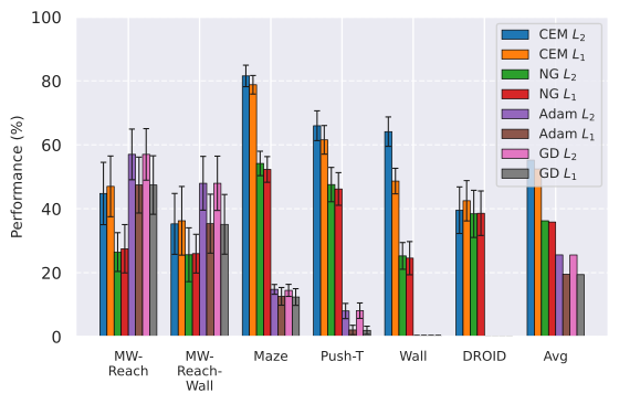
CEM with squared-distance cost is strongest overall, while Adam is especially effective on smoother Metaworld objectives. Gradient methods struggle with non-greedy obstacle and manipulation landscapes. Nevergrad is competitive on some robot-data settings with less tuning. No single optimizer wins uniformly.
Multistep rollout predictor training.
A short rollout-training horizon helps several tasks, but longer training rollouts can reduce one-step accuracy or alter data coverage. The appendix’s Lipschitz bounds explain potential error amplification rather than asserting that every actual error grows exponentially. Training and planning context choices must be interpreted together.
Impact of proprioception.
Measured state information improves precise goal reaching when visual patch features cannot resolve small displacements. Cross-domain transfer can invalidate proprioceptive coordinates, so the benefit does not transfer unchanged between DROID and RoboCasa.
Maximum context size.
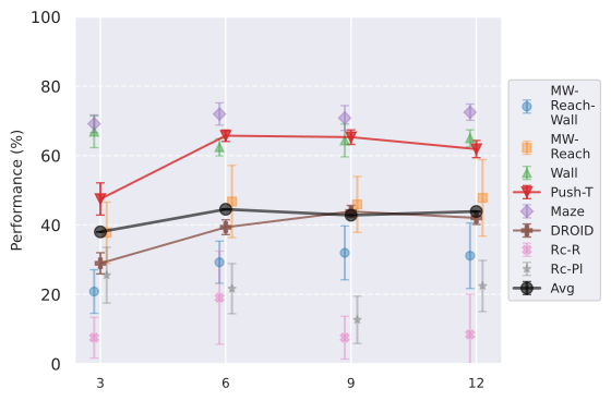
Two frames can supply motion information missing from a single image, but very long context does not consistently help. Deployment contexts longer than those seen in training can degrade rollouts. Larger context also changes the number and diversity of available training slices.
Encoder type.
DINO features are stronger in these controlled planning comparisons, and DINOv3 helps especially on photorealistic data. The proposed explanation concerns object boundaries and spatially localized changes. This is evidence for the examined frozen-feature planning setup, not a general ranking of all video-understanding or representation-learning tasks.
Predictor architecture.
Adaptive normalization with RoPE gives a useful average recipe, but differences are small and task-dependent; feature conditioning is best in some settings. Zero initialization and positional encoding do not produce a universal improvement. Matched action-ratio controls help separate conditioning from capacity.
Model scaling.
Simple simulated tasks often saturate or degrade with larger encoders and deeper predictors, while DROID benefits more consistently. Explanations include task complexity, harder latent optimization and fixed-compute undertraining. The study does not isolate one universal scaling mechanism.
Data scaling.
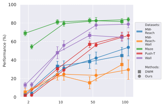
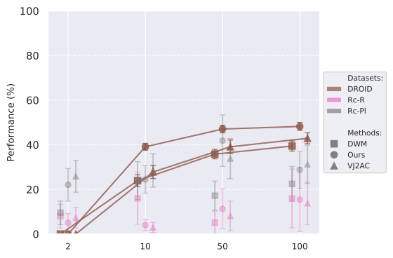
More data generally helps within the studied distributions, but transfer gains to RoboCasa are weaker because of domain shift. A larger training corpus cannot by itself guarantee camera, action or scene calibration in a new environment.
5.3 Our proposed optimum in the class of JEPA-WMs
The combined recipe uses short rollout training, appropriate context, selected image encoders and action conditioning, with smaller simulation models and larger photorealistic models. It improves most examined comparisons with DINO-WM and V-JEPA2-AC. Optimal here means best among the tested choices and tasks, not a theorem over all JEPA designs.
6 Conclusion
Planning outcomes emerge from representation, model training and search together. Deterministic regression is also a limitation when several futures are genuinely possible: predicting their conditional mean can be a poor physical future. Stochastic extensions and broader evaluation remain necessary beyond these largely deterministic benchmarks.
Broader Impact Statement
The impact statement discusses applications and risks of learned physical planning. The tested benchmarks do not certify safe deployment.
Author Contributions
The source specifies author contributions to methodology, implementation, experiments and writing. These disclosures remain separate from the evidence for individual design choices.
Acknowledgments
Acknowledgments and research support are retained as source context rather than treated as an additional result.
Appendix
The appendices retain the full implementation recipes, dataset definitions, planner algorithms, theoretical bounds, extra ablations and failure examples needed to qualify the main recommendations.
Appendix A Notation
The full symbol table defines training context, planning context, horizons, modalities and optimizer budgets. Distinguishing these quantities avoids conflating a longer training slice with a longer executed plan.
| Symbol | Description |
|---|---|
| Observations, actions and embeddings | |
| Observation (image frame) at time | |
| Action at time | |
| State embedding at time , i.e. | |
| Predicted state embedding at time | |
| Model components | |
| Encoder (visual, and optionally proprioceptive) | |
| Proprioceptive encoder | |
| Predictor | |
| Action encoder | |
| Predictor unrolling function (Equations 3 and 4) | |
| Planning evaluation function | |
| Parameters | |
| Encoder parameters (frozen) | |
| Learnable parameters (predictor, action encoder, proprioceptive encoder) | |
| Losses and objectives | |
| Teacher-forcing training loss (Equation 1) | |
| -step rollout loss (Equation 5) | |
| Planning objective (Equation 2) | |
| , | Visual and proprioceptive dissimilarity metrics |
| Proprioceptive loss weight in planning | |
| Dimensional and architectural parameters | |
| Embedding dimension of encoder / predictor | |
| Action dimension | |
| Frameskip factor | |
| Action embedding dimension (feature conditioning) | |
| Number of spatial patches of the visual encoder | |
| Training batch size | |
| Training parameters | |
| Maximum teacher-forcing context length at training time | |
| Maximum rollout context length at training time | |
| Planning parameters (see also Table 10) | |
| Maximum rollout context length at planning time | |
| Planning horizon (number of predicted steps) | |
| Number of candidate action trajectories | |
| Number of optimizer iterations | |
| Number of top trajectories retained (CEM) | |
| Number of planned actions stepped in environment | |
| Maximum number of steps per planning episode | |
Appendix B Extended Related Work
Alternative latent-space planning paradigms.
Locally linear models, control-oriented latent spaces and alternative latent planning methods impose different representations or objectives. The survey defines the narrower explicit JEPA-WM family studied here rather than subsuming every model-based controller.
Explicit and implicit world models.
Autoregressive latent predictors permit new rollout costs and search procedures at test time. Implicit predictive representations may encode longer-term structure without exposing the same explicit transition interface, changing what planning operations are available.
Reward- and reconstruction-based latent world models vs. JEPA-WMs.
Generative and reward-based latent models often jointly learn reconstruction, rewards, values or policies. Their success is not an isolated test of reconstruction-free next-embedding prediction, and the paper details those differences model by model.
Appendix C Training details
Predictor.
The appendix retains the exact predictor, action encoder and proprioceptive encoder optimization schedule. These settings make the controlled design comparisons reproducible.
Action conditioning of the predictor.
Feature concatenation, action-token concatenation, AdaLN and AdaLN-zero distribute conditioning differently across dimensions and layers. The complete architectural definitions prevent treating the labels as equivalent implementations.
| Hyperparameter | WM | WM-L | WM-V |
|---|---|---|---|
| data | |||
| 3 | 3 | 3 | |
| 5 | - | - | |
| resolution | 224 | 224 | 256 |
| optimization | |||
| lr | 5e-4 | - | - |
| start_weight_decay | 1e-7 | - | - |
| final_weight_decay | 1e-6 | - | - |
| AdamW | 0.9 | - | - |
| AdamW | 0.995 | - | - |
| clip_grad | 1 | - | - |
| architecture | |||
| patch_size | 14 | - | 16 |
| pred_depth | 6 | - | - |
| pred_embed_dim | 384 | 1024 | 1024 |
| enc_embed_dim | 384 | 1024 | 1024 |
| hardware | |||
| dtype | bfloat16 | - | - |
| accelerator | H100 80G | - | - |
| Hyperparameter | Metaworld | Push-T | Maze | Wall | DROID |
| optimization | |||||
| batch_size | 256 | 256 | 128 | 128 | 128 |
| epochs | 50 | 50 | 50 | 50 | 315 |
| architecture | |||||
| action_dim | 20 | 10 | 10 | 10 | 7 |
| action_embed_dim | 20 | 10 | 10 | 10 | 10 |
| proprio_dim | 4 | 4 | 4 | 4 | 7 |
| proprio_embed_dim | 20 | 20 | 20 | 10 | 10 |
Train time.
Measured per-epoch times expose training-cost differences across models and datasets. They are tied to the stated hardware and data pipeline.
| Model | Metaworld | Push-T | Maze | Wall | DROID |
|---|---|---|---|---|---|
| 1-step | 23 | 48 | 5 | 1 | 7 |
| 2-step | 23 | 49 | 5 | 1 | 8 |
| 3-step | 23 | 50 | 5 | 1 | 9 |
| 6-step | 30 | 64 | 16 | 2 | 17 |
| 20 | 42 | 5 | 1 | 13 | |
| WM-B | 23 | 50 | 5 | 1 | 8 |
| WM-L | 25 | 50 | 5 | 1 | 8 |
| WM-prop | 24 | 50 | 5 | 1 | 7 |
| WM-V | 25 | 60 | 7 | 2 | 9 |
Visual decoder.
A separately trained visual decoder reconstructs each encoder’s representations for diagnostic plots. Decoder quality and perceptual loss can affect apparent image fidelity, so the visualization does not directly measure task success.
State decoder.
A supervised state decoder probes physical variables from frozen features. It allows evaluating represented state along imagined rollouts but does not add those labels to the main predictive training objective.
V-JEPA-2-AC reproduction.
The reproduction identifies and corrects a particular rollout-loss indexing issue in the referenced action-conditioned implementation. Reported reproduction settings and fixes matter; this finding should not be generalized into a claim that all V-JEPA2 results are invalid.
Data augmentation ablations.
Cropping and image aspect ratios affect which scene information remains visible. The augmentation ablations distinguish realistic robot-data preprocessing from synthetic square images.
Ablations on models trained with video encoders.
Video encoder frame duplication and loss choices are explicitly tested before selecting the comparative recipe. The result depends on that adaptation; it is not a proof that video pretraining cannot support good control.
Encoder comparison details.
Token counts, patch sizes and preprocessing are documented along with encoder weights. Equal token counts improve comparability but do not make the pretrained data and objectives identical.
| Configuration | DINOv2 ViT-L | DINOv3 ViT-L | V-JEPA ViT-L | V-JEPA2 ViT-L |
|---|---|---|---|---|
| Encoder Architecture | ||||
| Encoder type | Image | Image | Video | Video |
| Model size | ViT-L/14 | ViT-L/16 | ViT-L/16 | ViT-L/16 |
| Patch embedding | Conv2d(14, 14) | Conv2d(16, 16) | Conv3d(2, 16, 16) | Conv3d(2, 16, 16) |
| Embedding dimension | 1024 | 1024 | 1024 | 1024 |
| Patches per timestep | ||||
| Input normalization | ImageNet stats | ImageNet stats | ImageNet stats | ImageNet stats |
| Positional encoding | Sincos | RoPE | Sincos | RoPE |
| Attention mask | Full | Full | Full | Full |
| Input Preprocessing | ||||
| Input resolution | ||||
| Input frame count | 1 per timestep | 1 per timestep | 2 per timestep | 2 per timestep |
| Frame duplication | No | No | Yes (duplicate each) | Yes (duplicate each) |
Multistep rollout variants ablations.
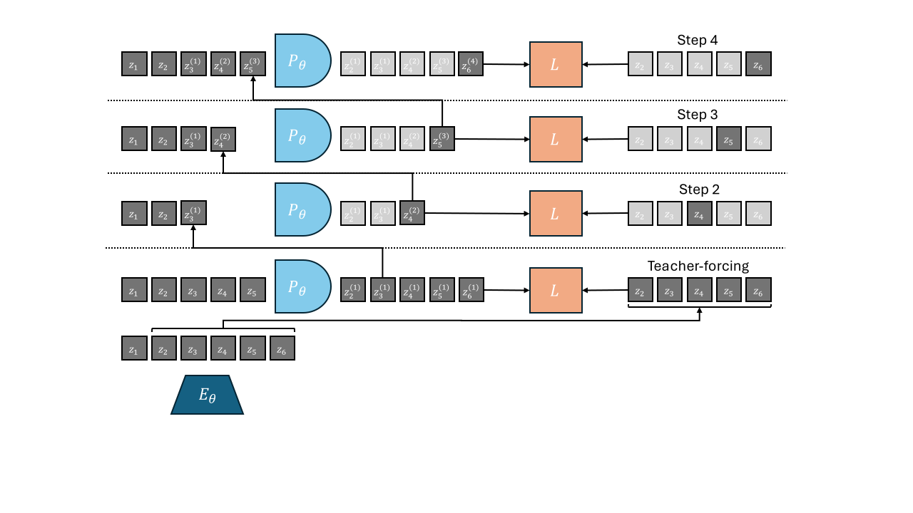
Several teacher-forced and self-fed context variants change where prediction errors are measured and where derivatives stop. The diagrams retain the precise schedules, because a nominal two-step rollout loss can otherwise refer to materially different procedures.
Appendix D Error propagation in autoregressive latent prediction
A recurrence bounds rollout error by accumulated one-step error amplified through the predictor’s Lipschitz constant. The upper bound is geometric for an expansive predictor, linear when the constant equals one and bounded when contractive. Tight examples and stronger lower-bound assumptions are distinguished from a universal claim of exponential observed error. Context windows, training error and robustness create additional tradeoffs.
Equations 6–17
| (6) |
| (7) |
| (8) |
| (9) |
| (10) |
| (11) |
| (12) |
| (13) |
| (14) |
| (15) |
| (16) |
| (17) |
Appendix E Planning environments and datasets
Actions and proprioception are normalized per dataset and denormalized for execution. Shared parameter shapes do not imply shared physical coordinates across datasets.
Data slicing.
Splitting occurs by trajectories before constructing temporal slices, reducing adjacent-frame leakage across train and validation. Slice length and stride change training coverage as context grows.
| Dataset Size | Traj. Len. | |
|---|---|---|
| PointMaze | 2000 | 100 |
| Push-T | 18500 | 100-300 |
| Wall | 1920 | 50 |
| Metaworld | 12600 | 100 |
| DROID | 8000 | 20-50 |
DROID.
DROID uses measured pose deltas and selected exterior camera views rather than joint multi-view input. Its offline action comparison is sensitive to coordinate and action calibration.
Robocasa.
RoboCasa provides simulated household manipulation for transfer from DROID-trained models. Camera and action-domain differences can make a plausible predicted movement physically inaccurate in the new simulator.
Metaworld.
Metaworld data is gathered with trained agents across the listed tasks. Evaluation includes pose-reaching and object-interaction settings, whose requirements differ despite sharing the same model family.
| Task | Description |
|---|---|
| turn on faucet | Rotate the faucet counter-clockwise. Randomize faucet positions |
| sweep | Sweep a puck off the table. Randomize puck positions |
| assemble nut | Pick up a nut and place it onto a peg. Randomize nut and peg positions |
| turn off faucet | Rotate the faucet clockwise. Randomize faucet positions |
| push | Push the puck to a goal. Randomize puck and goal positions |
| pull lever | Pull a lever down degrees. Randomize lever positions |
| push with stick | Grasp a stick and push a box using the stick. Randomize stick positions. |
| get coffee | Push a button on the coffee machine. Randomize the position of the coffee machine |
| pull handle side | Pull a handle up sideways. Randomize the handle positions |
| pull with stick | Grasp a stick and pull a box with the stick. Randomize stick positions |
| disassemble nut | pick a nut out of the a peg. Randomize the nut positions |
| place onto shelf | pick and place a puck onto a shelf. Randomize puck and shelf positions |
| press handle side | Press a handle down sideways. Randomize the handle positions |
| hammer | Hammer a screw on the wall. Randomize the hammer and the screw positions |
| slide plate | Slide a plate into a cabinet. Randomize the plate and cabinet positions |
| slide plate side | Slide a plate into a cabinet sideways. Randomize the plate and cabinet positions |
| press button wall | Bypass a wall and press a button. Randomize the button positions |
| press handle | Press a handle down. Randomize the handle positions |
| pull handle | Pull a handle up. Randomize the handle positions |
| soccer | Kick a soccer into the goal. Randomize the soccer and goal positions |
| retrieve plate side | Get a plate from the cabinet sideways. Randomize plate and cabinet positions |
| retrieve plate | Get a plate from the cabinet. Randomize plate and cabinet positions |
| close drawer | Push and close a drawer. Randomize the drawer positions |
| press button top | Press a button from the top. Randomize button positions |
| reach | reach a goal position. Randomize the goal positions |
| press button top wall | Bypass a wall and press a button from the top. Randomize button positions |
| reach with wall | Bypass a wall and reach a goal. Randomize goal positions |
| insert peg side | Insert a peg sideways. Randomize peg and goal positions |
| pull | Pull a puck to a goal. Randomize puck and goal positions |
| push with wall | Bypass a wall and push a puck to a goal. Randomize puck and goal positions |
| pick out of hole | Pick up a puck from a hole. Randomize puck and goal positions |
| pick&place w/ wall | Pick a puck, bypass a wall and place the puck. Randomize puck and goal positions |
| press button | Press a button. Randomize button positions |
| pick&place | Pick and place a puck to a goal. Randomize puck and goal positions |
| unplug peg | Unplug a peg sideways. Randomize peg positions |
| close window | Push and close a window. Randomize window positions |
| open door | Open a door with a revolving joint. Randomize door positions |
| close door | Close a door with a revolving joint. Randomize door positions |
| open drawer | Open a drawer. Randomize drawer positions |
| close box | Grasp the cover and close the box with it. Randomize the cover and box positions |
| lock door | Lock the door by rotating the lock clockwise. Randomize door positions |
| pick bin | Grasp the puck from one bin and place it into another bin. Randomize puck positions |
Push-T.
Push-T requires accurate contact between a pusher and a T-shaped block. Small action-position errors can cause failure even when the visual future appears broadly plausible.
PointMaze.
PointMaze includes velocity and inertia in a force-actuated navigation task. Random start–goal tests require enough state information and search ability to navigate the layout.
Wall.
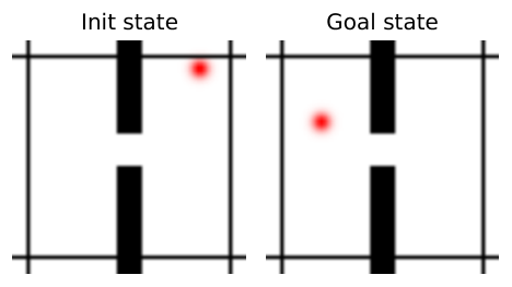
Wall requires moving through a doorway between rooms. Its non-greedy geometry tests whether a planner escapes directly goal-directed local minima.
Appendix F Planning Optimization
The same latent-goal objective is paired with several planning algorithms. Their complete pseudocode and budgets are retained so runtime and success comparisons can be assessed independently of model training.
Model Predictive Control.
The study uses repeated model-predictive replanning on Metaworld as specified; other reported protocols should not automatically be assumed to have the same feedback opportunities.
Cross-Entropy Method.
CEM samples time-indexed actions from a factorized Gaussian, ranks candidates and refits using elites. Its useful exploration depends on variance, population and stopping settings.
Equation


NG Planner.
The Nevergrad interface supplies the same predictive cost and a comparable evaluation budget. Its meta-optimizer selects a diagonal evolutionary strategy in these experiments, rather than an entirely fixed universal algorithm.
Gradient Descent Planner.
Gradient descent differentiates final goal distance through the latent rollout. It can refine smooth local paths efficiently but is sensitive to initialization and non-greedy local minima.
Adam Planner.
Adam changes the action optimizer’s directional scaling through moving gradient moments. It uses the same learned predictive objective, so changing the planner does not independently improve representation quality.
Planning hyperparameters.
Horizon, context, candidate population, elite count and iteration budgets are reported per environment. Success is sensitive to these settings even for an unchanged world model.
| PointMaze | 300 | 6 | 6 | 10 | 30 | 2 | 5 | 30 |
|---|---|---|---|---|---|---|---|---|
| Push-T | 300 | 6 | 6 | 10 | 30 | 2 | 5 | 30 |
| Wall | 300 | 6 | 6 | 10 | 30 | 2 | 5 | 30 |
| Metaworld | 300 | 6 | 3 | 10 | 15 | 2 | 5 | 100 |
| Robocasa | 300 | 3 | 1 | 10 | 15 | 2 | 5 | 60 |
| DROID | 300 | 3 | 3 | 10 | 15 | 2 | 1 |
Appendix G Additional experiments
G.1 Additional results
Equalized action ratio experiments.
Equalized action-to-visual ratios control a capacity confound in comparing conditioning schemes. Remaining preferences still depend on the task, limiting universal architecture conclusions.
Additional planner ablations.
Additional optimizer and seed tables test how the chosen combined recipe behaves across planners and initializations. Reproducibility at a checkpoint and stability across training are distinct forms of variability.
| Model | Planner | Maze | Wall | Push-T | MW-R | MW-RW | Rc-R | Rc-Pl | DROID |
|---|---|---|---|---|---|---|---|---|---|
| CEM | DWM | 81.6 (3.4) | 64.1 (4.6) | 66.0 (4.7) | 44.8 (8.9) | 35.1 (9.4) | 19.1 (13.4) | 21.7 (7.2) | 39.4 (2.1) |
| VJ2AC | — | — | — | — | — | 16.2 (8.3) | 33.1 (7.2) | 42.9 (2.5) | |
| Ours | 83.9 (2.3) | 78.8 (3.9) | 70.2 (2.8) | 58.2 (9.3) | 41.6 (10.0) | 25.4 (16.6) | 30.7 (8.0) | 48.2 (1.8) | |
| CEM | DWM | 78.8 (2.9) | 48.7 (4.0) | 61.6 (4.5) | 45.1 (10.4) | 34.0 (9.1) | 14.4 (11.3) | 19.6 (7.4) | 41.7 (2.7) |
| VJ2AC | — | — | — | — | — | 13.2 (10.3) | 30.9 (7.3) | 38.5 (5.7) | |
| Ours | 79.7 (3.1) | 46.7 (3.6) | 63.4 (2.1) | 55.1 (8.5) | 40.8 (9.2) | 17.6 (12.3) | 30.5 (8.7) | 47.2 (1.8) | |
| NG | DWM | 54.2 (3.8) | 25.3 (4.2) | 47.6 (5.4) | 28.1 (7.8) | 27.9 (10.0) | 25.8 (16.7) | 27.1 (8.6) | 36.0 (3.6) |
| VJ2AC | — | — | — | — | — | 22.1 (8.9) | 31.1 (7.0) | 36.2 (3.2) | |
| Ours | 72.7 (4.5) | 35.4 (5.9) | 48.0 (3.0) | 29.3 (8.6) | 21.0 (7.7) | 30.5 (10.7) | 36.9 (9.1) | 39.9 (1.9) | |
| NG | DWM | 52.3 (4.0) | 24.6 (5.2) | 46.2 (5.1) | 27.5 (8.5) | 28.6 (8.9) | 21.6 (15.5) | 26.0 (8.0) | 35.4 (3.3) |
| VJ2AC | — | — | — | — | — | 18.4 (11.8) | 29.4 (5.1) | 33.7 (3.9) | |
| Ours | 69.5 (2.1) | 30.9 (4.1) | 48.2 (5.1) | 27.8 (8.2) | 21.3 (8.9) | 25.7 (12.0) | 32.0 (9.9) | 40.0 (2.2) | |
| Adam | DWM | 14.8 (1.5) | 0.1 (0.3) | 8.0 (2.4) | 62.0 (8.3) | 49.9 (9.9) | 2.8 (3.7) | 21.5 (8.6) | 0.0 (0.0) |
| VJ2AC | — | — | — | — | — | 0.0 (0.0) | 5.9 (5.1) | 0.0 (0.0) | |
| Ours | 17.7 (3.3) | 1.1 (1.1) | 9.0 (2.1) | 55.3 (9.9) | 39.7 (9.7) | 0.0 (0.0) | 10.5 (5.0) | 0.0 (0.0) | |
| Adam | DWM | 12.6 (2.8) | 0.1 (0.3) | 2.1 (1.5) | 50.7 (8.5) | 37.2 (8.3) | 0.9 (1.4) | 22.1 (7.5) | 0.0 (0.0) |
| VJ2AC | — | — | — | — | — | 0.0 (0.0) | 3.5 (2.8) | 0.0 (0.0) | |
| Ours | 16.1 (3.5) | 0.0 (0.2) | 0.9 (0.9) | 53.2 (7.4) | 43.1 (6.4) | 0.2 (0.7) | 7.5 (3.9) | 0.0 (0.0) | |
| GD | DWM | 14.5 (1.9) | 0.1 (0.3) | 8.1 (2.4) | 62.2 (8.2) | 50.0 (10.1) | 2.9 (3.8) | 21.9 (8.4) | 0.0 (0.0) |
| VJ2AC | — | — | — | — | — | 0.0 (0.0) | 8.1 (3.6) | 0.0 (0.0) | |
| Ours | 17.7 (3.3) | 1.1 (1.1) | 9.1 (1.9) | 55.3 (9.9) | 39.7 (9.7) | 0.0 (0.0) | 10.5 (5.0) | 0.0 (0.0) | |
| GD | DWM | 12.4 (2.6) | 0.1 (0.3) | 2.0 (1.3) | 50.9 (8.5) | 37.1 (8.4) | 1.0 (1.4) | 22.2 (7.3) | 0.0 (0.0) |
| VJ2AC | — | — | — | — | — | 0.0 (0.0) | 4.0 (2.6) | 0.0 (0.0) | |
| Ours | 16.1 (3.5) | 0.0 (0.2) | 0.9 (0.9) | 53.3 (7.3) | 40.1 (12.3) | 0.2 (0.7) | 7.5 (3.9) | 0.0 (0.0) |
| Model | Planner | Maze | Wall | Push-T | MW-R | MW-RW | Rc-R | Rc-Pl | DROID |
|---|---|---|---|---|---|---|---|---|---|
| CEM | DWM | 79.2 (2.9) | 63.1 (2.3) | 63.3 (3.9) | 44.4 (5.5) | 31.9 (2.6) | 11.5 (7.8) | 20.8 (9.7) | 40.4 (1.6) |
| VJ2AC | — | — | — | — | — | 7.3 (6.4) | 33.3 (5.9) | 43.2 (1.9) | |
| Ours | 83.3 (3.1) | 80.9 (4.9) | 69.4 (4.0) | 49.0 (9.4) | 29.2 (11.5) | 22.9 (21.4) | 34.4 (7.7) | 46.5 (0.4) | |
| CEM | DWM | 78.3 (2.1) | 50.0 (3.7) | 60.6 (2.2) | 49.3 (5.5) | 38.2 (10.4) | 13.5 (8.2) | 14.6 (5.3) | 41.6 (1.8) |
| VJ2AC | — | — | — | — | — | 8.3 (3.9) | 31.2 (6.8) | 40.9 (3.1) | |
| Ours | 81.2 (4.7) | 47.6 (2.1) | 55.9 (3.0) | 48.4 (10.7) | 30.7 (7.0) | 20.8 (22.9) | 29.2 (11.8) | 45.0 (0.3) | |
| NG | DWM | 55.6 (2.3) | 25.2 (4.3) | 48.8 (3.0) | 25.7 (2.0) | 27.1 (1.7) | 20.8 (7.8) | 33.3 (8.2) | 35.4 (2.2) |
| VJ2AC | — | — | — | — | — | 18.8 (4.4) | 29.2 (2.9) | 35.7 (2.1) | |
| Ours | 76.4 (0.5) | 38.9 (4.2) | 49.7 (2.7) | 23.4 (8.4) | 13.0 (5.6) | 26.0 (16.6) | 35.4 (6.4) | 39.8 (0.7) | |
| NG | DWM | 52.3 (2.0) | 23.1 (6.6) | 42.1 (4.4) | 31.2 (6.1) | 29.2 (3.4) | 24.0 (8.2) | 28.1 (15.9) | 38.4 (3.2) |
| VJ2AC | — | — | — | — | — | 9.4 (2.6) | 28.1 (2.6) | 34.0 (4.9) | |
| Ours | 73.6 (3.0) | 30.6 (1.3) | 43.8 (0.9) | 27.6 (6.5) | 12.5 (6.4) | 18.8 (19.9) | 32.3 (12.6) | 39.9 (1.3) | |
| Adam | DWM | 14.6 (3.1) | 0.0 (0.0) | 8.9 (0.5) | 60.4 (2.9) | 44.4 (7.7) | 7.3 (2.9) | 24.0 (10.3) | 0.0 (0.0) |
| VJ2AC | — | — | — | — | — | 0.0 (0.0) | 12.5 (5.1) | 0.0 (0.0) | |
| Ours | 21.5 (4.2) | 1.0 (0.9) | 8.3 (0.9) | 45.8 (3.9) | 25.5 (10.6) | 3.1 (3.1) | 9.4 (3.1) | 0.0 (0.0) | |
| Adam | DWM | 12.0 (1.6) | 0.0 (0.0) | 3.1 (1.0) | 45.8 (6.8) | 34.7 (5.2) | 3.1 (4.4) | 21.9 (0.0) | 0.0 (0.0) |
| VJ2AC | — | — | — | — | — | 0.0 (0.0) | 4.2 (1.5) | 0.0 (0.0) | |
| Ours | 17.7 (1.5) | 0.0 (0.0) | 1.0 (0.0) | 45.8 (2.6) | 33.9 (3.1) | 0.0 (0.0) | 7.8 (4.7) | 0.0 (0.0) | |
| GD | DWM | 13.5 (2.1) | 0.0 (0.0) | 8.3 (1.0) | 61.8 (2.0) | 45.8 (6.8) | 7.3 (2.9) | 25.0 (9.2) | 0.0 (0.0) |
| VJ2AC | — | — | — | — | — | 0.0 (0.0) | 5.2 (1.5) | 0.0 (0.0) | |
| Ours | 21.5 (4.2) | 1.0 (0.9) | 8.3 (0.9) | 45.8 (3.9) | 25.5 (10.6) | 3.1 (3.1) | 9.4 (3.1) | 0.0 (0.0) | |
| GD | DWM | 12.0 (1.6) | 0.0 (0.0) | 2.1 (0.0) | 45.8 (6.8) | 34.7 (5.2) | 3.1 (4.4) | 21.9 (0.0) | 0.0 (0.0) |
| VJ2AC | — | — | — | — | — | 0.0 (0.0) | 4.2 (1.5) | 0.0 (0.0) | |
| Ours | 17.7 (1.5) | 0.0 (0.0) | 1.0 (0.0) | 45.8 (2.6) | 33.9 (3.1) | 0.0 (0.0) | 7.8 (4.7) | 0.0 (0.0) |

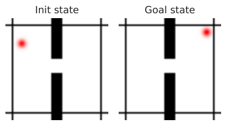

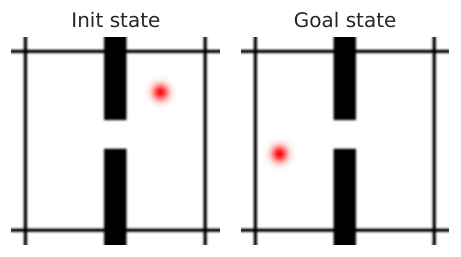
Object manipulation on Robocasa and DROID.
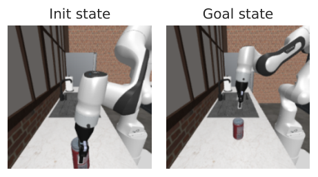
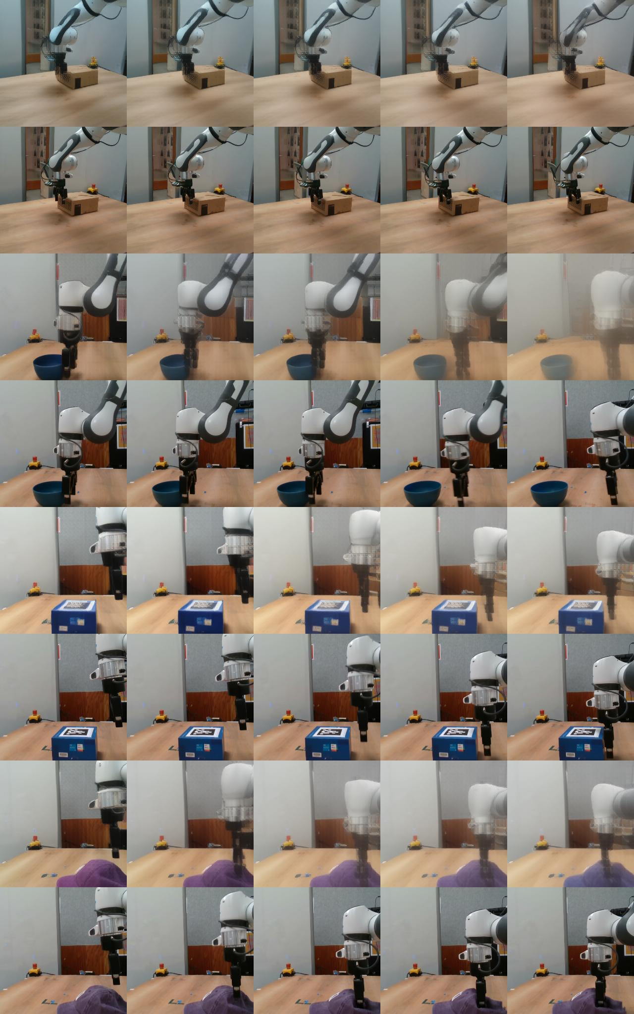
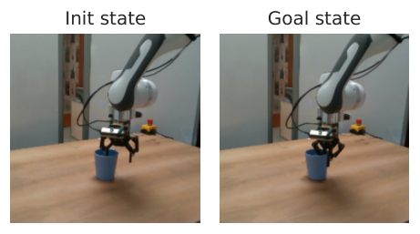
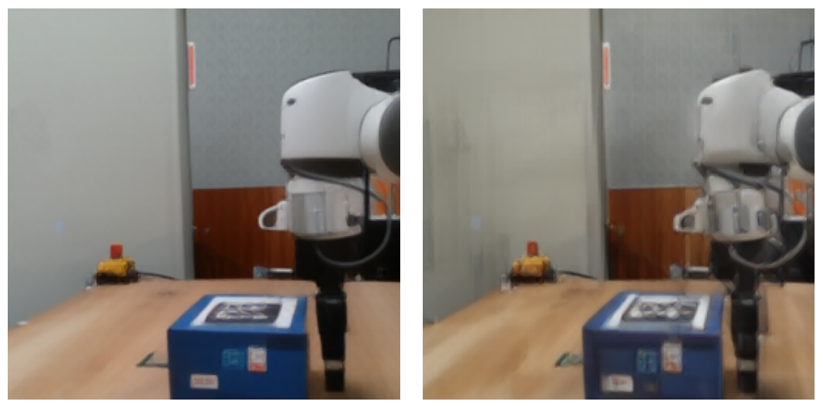
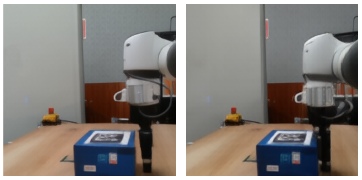
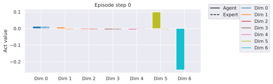
Selected RoboCasa and DROID examples expose calibration errors and differing success on reaching, placing and picking. A favorable latent objective can coexist with the wrong physical arm location.
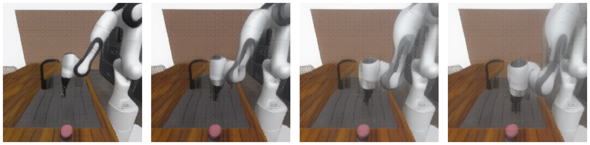

Object manipulation on Metaworld.
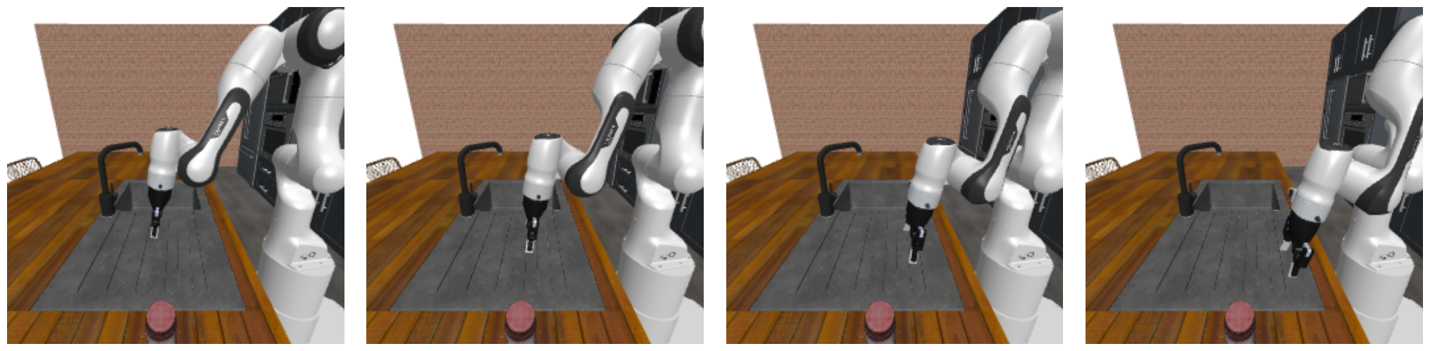
In Metaworld, the model can imagine grasping an object when execution does not grasp it. These failure examples separate visual plausibility and interaction modeling from actual controlled outcome.



 |
 |
Action precision Push-T.
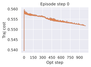
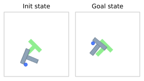
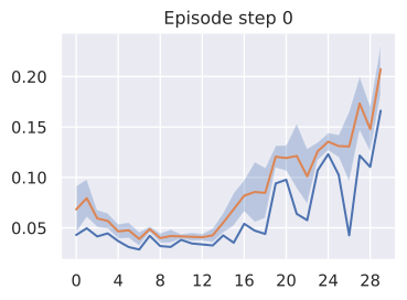
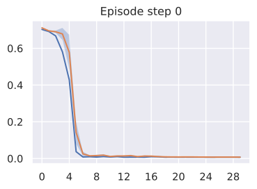
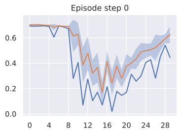
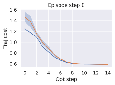
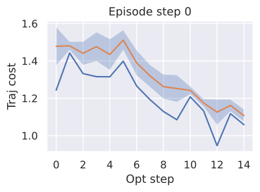
Push-T needs precise final actions, favoring convergence before execution. Nevergrad can explore useful alternatives yet remain less precise than CEM under the stated budgets.
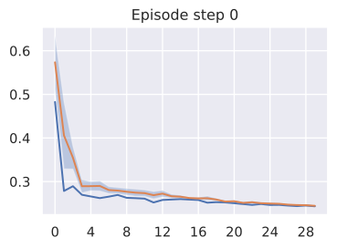
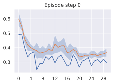
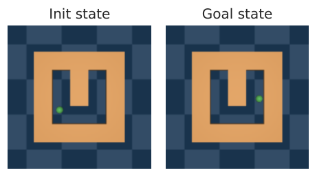
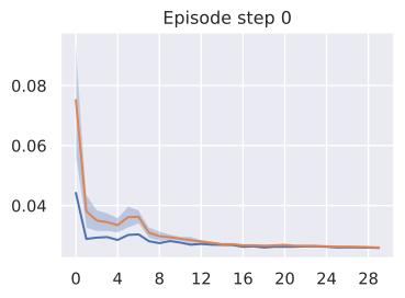
Embedding space and model size.
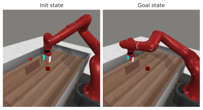
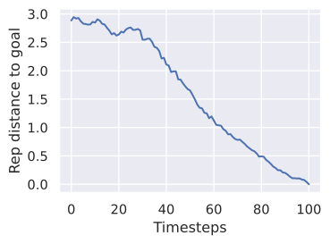
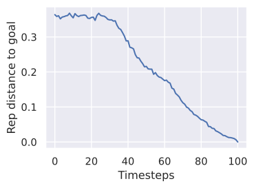
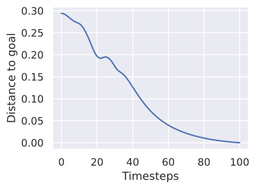
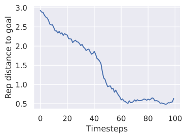
A larger feature space can make relative goal-distance differences smaller. This can complicate optimization despite greater representation capacity, providing one explanation for why scaling is task-dependent.
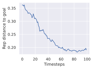
G.2 Evaluation metrics
Statistical significance.
The statistical protocol averages multiple task pairs and training checkpoints and reports seed variability where available. Correlated checkpoints should not be mistaken for fully independent training runs.
Embedding space error throughout unrolling.
Latent prediction error is evaluated at several autoregressive horizons on validation trajectories. It measures the forecasting problem on those trajectories rather than whether an optimizer can solve a new goal.
Proprioceptive decoding error throughout unrolling.
A fixed state decoder maps imagined latents to physical-state predictions, testing rollout content with a supervised probe. Its own approximation error limits interpretation.
Visual decoder.
Visual decoders act frame by frame to reduce artificial temporal consistency from a powerful decoder. Reconstructed video remains a diagnostic rather than direct proof of the model’s physical accuracy.
Action error.
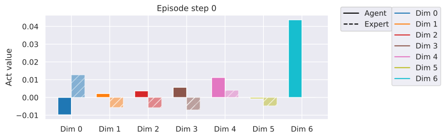
Offline action error compares one planned command sequence with a recorded one. Multiple action sequences may reach the same goal, and out-of-distribution action magnitudes can distort this proxy.
G.3 Is there a proxy for success rate?
Validation losses correlate with success inconsistently across tasks and planners. Forecasting under held-out trajectories differs from goal-directed search, whose optimizer can exploit out-of-distribution actions or get stuck. The study therefore retains direct control evaluation rather than treating any single loss as a universal success proxy.
| Model name | WM | WM-prop | WM-2-step | WM-L | Mean | |
|---|---|---|---|---|---|---|
| Proprio dec | 0.40 | 0.44 | 0.40 | 0.26 | 0.20 | 0.34 |
| Proprio dec | 0.41 | 0.34 | 0.45 | 0.27 | 0.21 | 0.34 |
| Proprio dec | 0.38 | 0.44 | 0.40 | 0.33 | 0.18 | 0.35 |
| Vis emb | 0.44 | 0.51 | 0.62 | 0.39 | 0.23 | 0.44 |
| Vis emb | 0.42 | 0.46 | 0.62 | 0.39 | 0.24 | 0.42 |
| Vis emb | 0.36 | 0.44 | 0.59 | 0.37 | 0.20 | 0.39 |
| Vis emb | 0.45 | 0.55 | 0.69 | 0.41 | 0.24 | 0.47 |
| Vis emb | 0.45 | 0.52 | 0.72 | 0.43 | 0.25 | 0.47 |
| Vis emb | 0.42 | 0.52 | 0.72 | 0.42 | 0.22 | 0.46 |
| SR | 29.7 ±3.8 | 24.9 ±7.6 | 39.2 ±4.1 | 28.7 ±5.8 | 19.4 ±5.8 |
| Model name | WM | WM-prop | WM-2-step | WM-L | Mean | |
|---|---|---|---|---|---|---|
| Proprio dec | 0.70 | 0.73 | 0.85 | 0.71 | 0.81 | 0.76 |
| Proprio dec | 0.78 | 0.66 | 0.87 | 0.79 | 0.84 | 0.79 |
| Proprio dec | 0.76 | 0.70 | 0.78 | 0.83 | 0.86 | 0.79 |
| Vis emb | 0.80 | 0.73 | 0.88 | 0.82 | 0.87 | 0.82 |
| Vis emb | 0.85 | 0.76 | 0.91 | 0.84 | 0.87 | 0.85 |
| Vis emb | 0.86 | 0.70 | 0.89 | 0.80 | 0.87 | 0.82 |
| Vis emb | 0.87 | 0.79 | 0.92 | 0.83 | 0.90 | 0.86 |
| Vis emb | 0.88 | 0.78 | 0.93 | 0.84 | 0.88 | 0.86 |
| Vis emb | 0.87 | 0.75 | 0.91 | 0.83 | 0.87 | 0.85 |
| Model name | WM | WM-prop | WM-2-step | WM-3-step | WM-L | Mean | |
|---|---|---|---|---|---|---|---|
| Proprio dec | 0.25 | 0.38 | 0.19 | 0.23 | 0.26 | 0.16 | 0.25 |
| Proprio dec | 0.23 | 0.51 | 0.22 | 0.30 | 0.14 | 0.28 | 0.28 |
| Proprio dec | 0.22 | 0.49 | 0.39 | 0.26 | 0.34 | 0.23 | 0.32 |
| Vis emb | 0.72 | 0.94 | 0.74 | 0.73 | 0.69 | 0.75 | 0.76 |
| Vis emb | 0.69 | 0.94 | 0.69 | 0.70 | 0.61 | 0.74 | 0.73 |
| Vis emb | 0.68 | 0.94 | 0.65 | 0.69 | 0.56 | 0.70 | 0.70 |
| Vis emb | 0.78 | 0.96 | 0.81 | 0.77 | 0.73 | 0.80 | 0.81 |
| Vis emb | 0.74 | 0.96 | 0.76 | 0.72 | 0.69 | 0.79 | 0.78 |
| Vis emb | 0.73 | 0.96 | 0.73 | 0.72 | 0.64 | 0.75 | 0.75 |
| Model name | WM | WM-prop | WM-2-step | WM-3-step | WM-L | Mean | |
|---|---|---|---|---|---|---|---|
| Proprio dec | 0.15 | 0.19 | 0.15 | 0.14 | 0.25 | 0.09 | 0.16 |
| Proprio dec | 0.13 | 0.21 | 0.10 | 0.35 | 0.23 | 0.21 | 0.21 |
| Proprio dec | 0.10 | 0.34 | 0.25 | 0.10 | 0.27 | 0.10 | 0.19 |
| Vis emb | 0.43 | 0.50 | 0.82 | 0.53 | 0.42 | 0.19 | 0.48 |
| Vis emb | 0.23 | 0.24 | 0.74 | 0.50 | 0.53 | 0.03 | 0.38 |
| Vis emb | 0.21 | 0.30 | 0.67 | 0.46 | 0.49 | 0.17 | 0.38 |
| Vis emb | 0.58 | 0.68 | 0.86 | 0.54 | 0.38 | 0.36 | 0.57 |
| Vis emb | 0.37 | 0.49 | 0.78 | 0.55 | 0.50 | 0.19 | 0.48 |
| Vis emb | 0.29 | 0.38 | 0.74 | 0.51 | 0.50 | 0.29 | 0.45 |
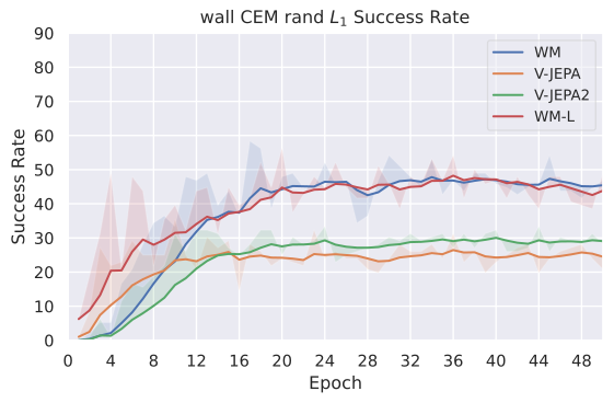
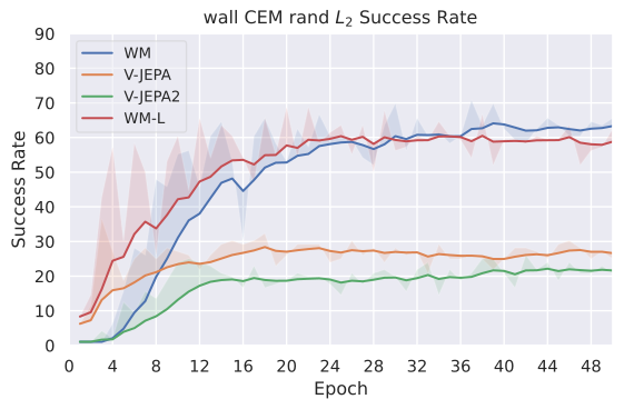
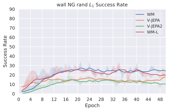
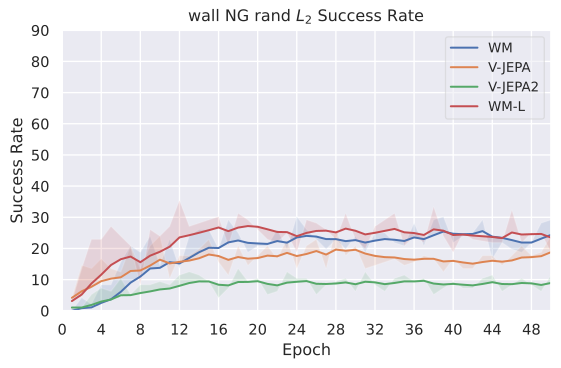
G.4 Success over epochs
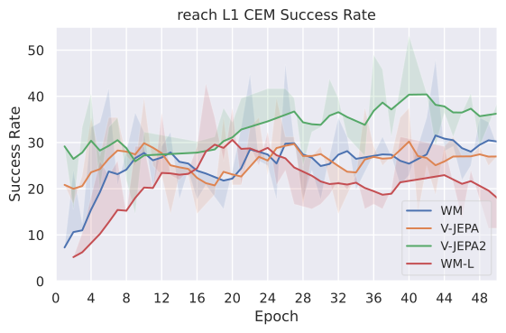
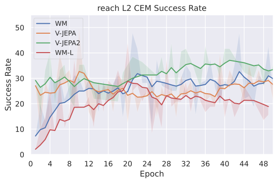
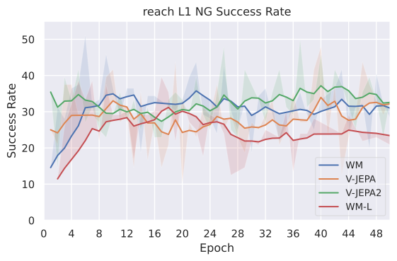
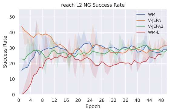
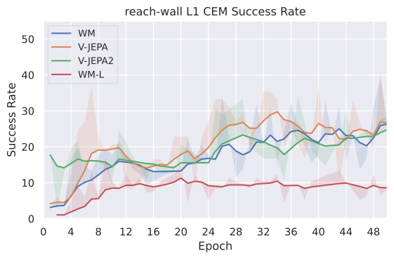
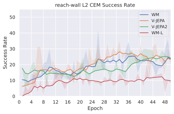
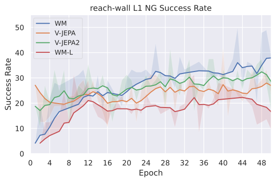
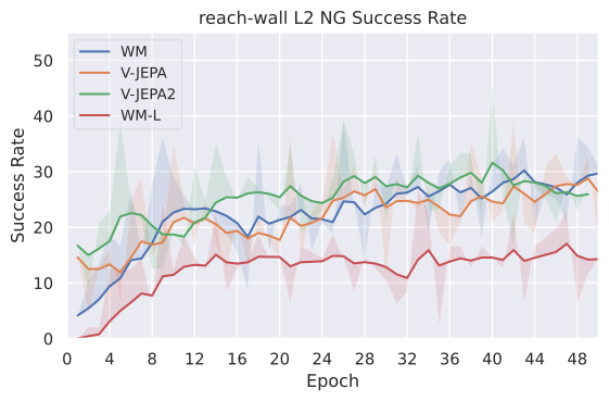
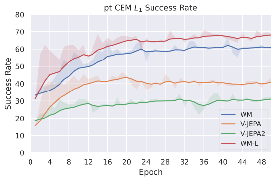
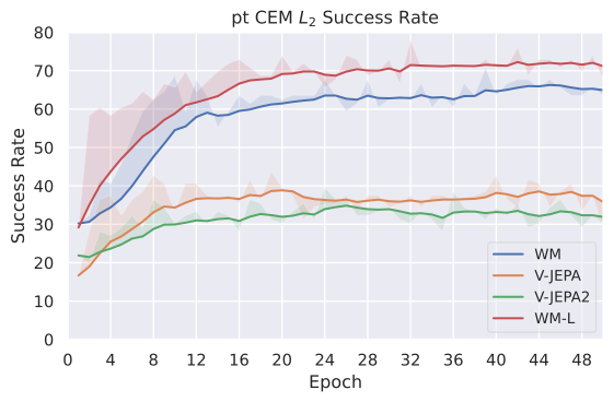
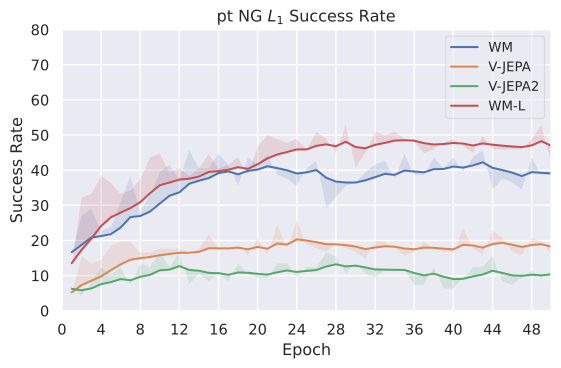
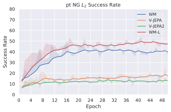
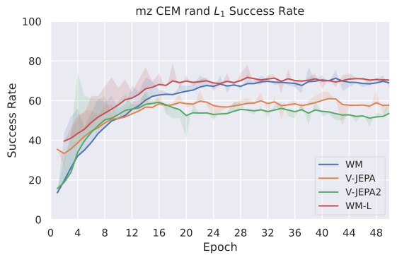
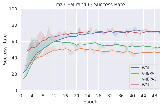
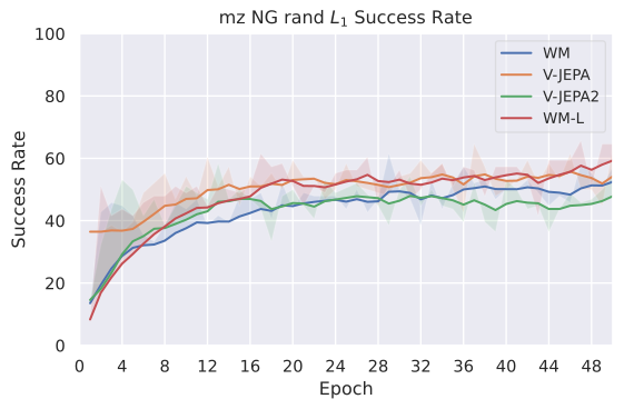
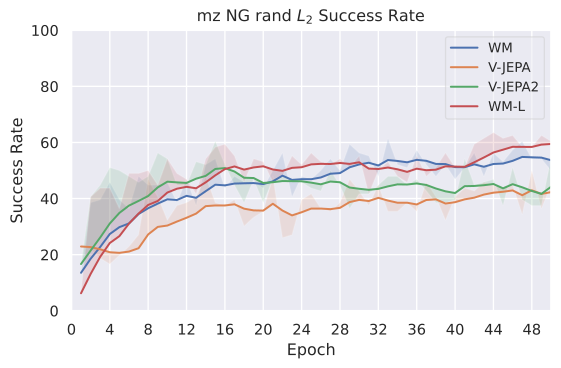
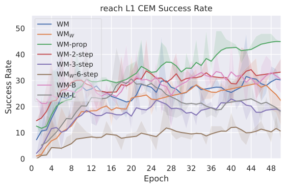
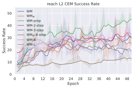
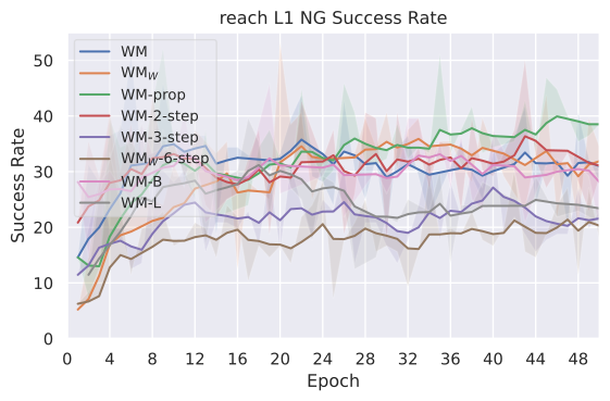
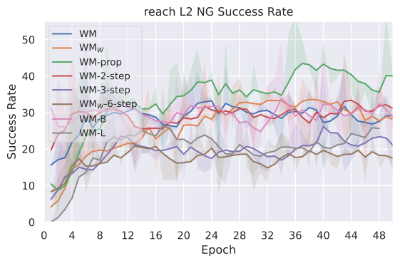
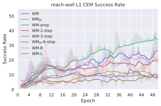
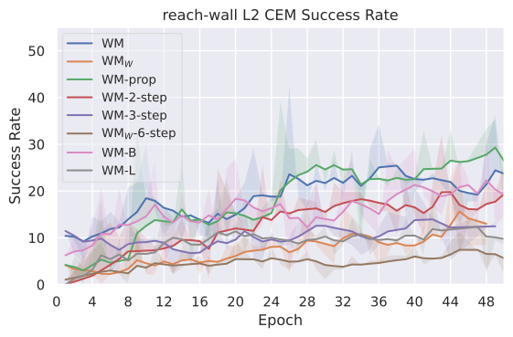
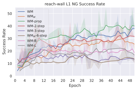
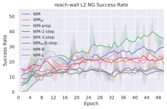
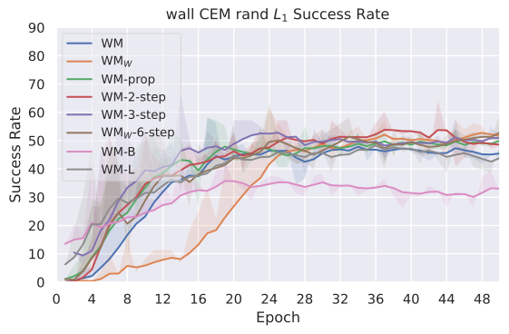
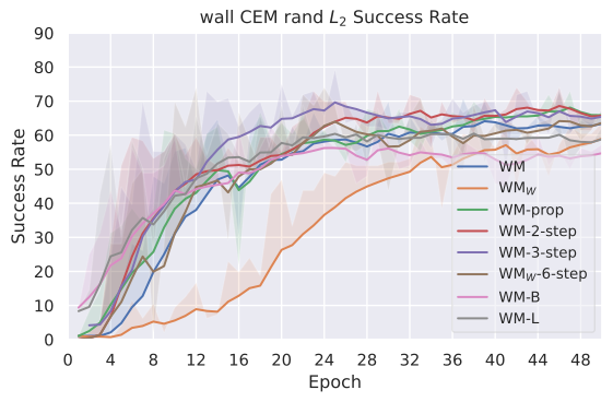
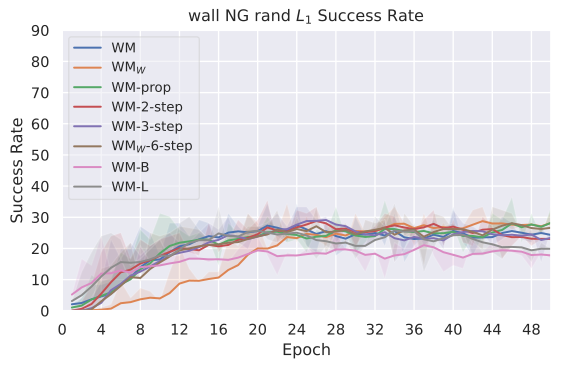
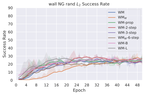
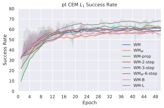
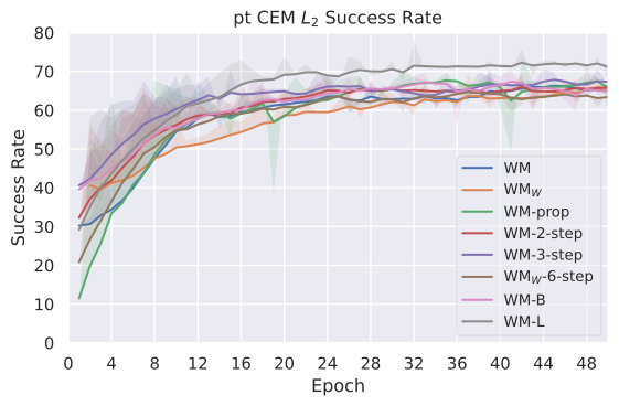
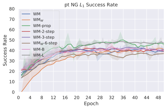
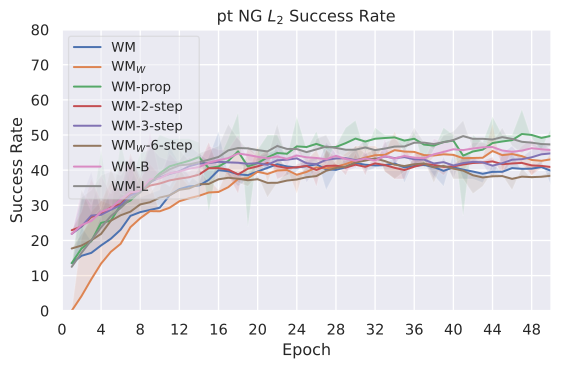
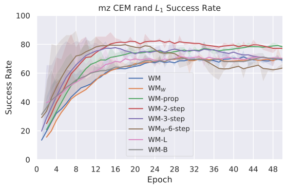
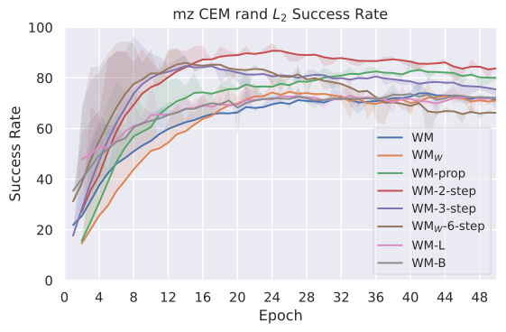
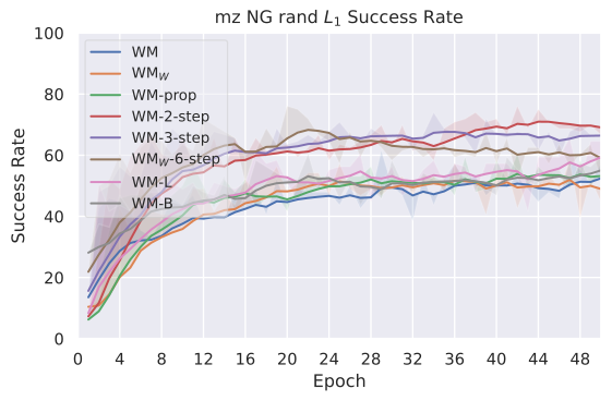
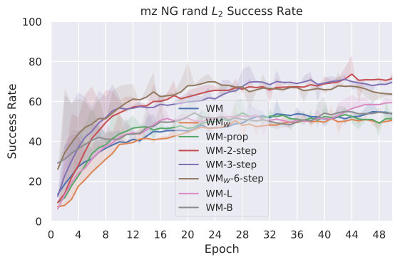
The complete success-over-training grids retain favorable and unfavorable dynamics across tasks, encoders and rollout settings. They contextualize final averages and expose instability hidden by a single checkpoint.