At a glance
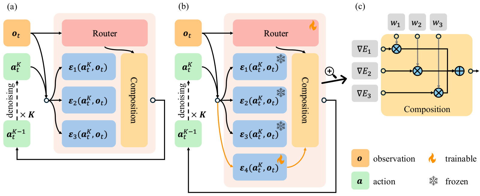
FDP learns several diffusion-policy components jointly and combines their denoising predictions using observation-dependent weights. The aim is to model varied robot behaviors and adapt to new tasks by tuning a small subset of parameters or adding a component.
Simulation and four physical manipulation tasks support improved average performance and efficient adaptation. Freezing old components alone does not prevent forgetting: the encoder and router can still change, and a small replay buffer substantially improves retention.
Introduction
A single policy can struggle to represent varied manipulation behaviors. FDP distributes modeling across diffusion components and continuously combines their outputs, instead of selecting a few experts through discrete routing. New tasks can reuse old components and add a copied, trainable component.
The experiments study multitask success, adaptation, scaling, and component behavior. The evidence supports a useful modular architecture; it does not establish fully independent, uniquely identifiable skills.
Related Works
The design connects diffusion-based action generation with modular multitask policies.
II- 1 Diffusion Models for Robotics
Diffusion models generate actions or trajectories by repeatedly denoising a sample. Prior work applies them to visuomotor control, planning, grasping, and bimanual manipulation. FDP builds on Diffusion Policy and compositional diffusion modeling. [10]
II- 2 Multitask Imitation Learning and Adaptation
SDP routes among experts using observations, while MoDE routes according to diffusion noise level. FDP combines complete diffusion components continuously and trains every component on each update. This avoids hard selection in its training design; qualitative analyses examine whether meaningful behavior specialization emerges.
FDP : Factorized Diffusion Policy
The policy factorizes an observation-conditioned action distribution into weighted component distributions. A learned router determines how strongly each component contributes at each observation.
Probabilistic Policy Modeling
Multiplying powered component densities favors actions compatible with their combined preferences. Each component is represented through a diffusion denoiser. The product-of-distributions view motivates interpreting components as soft behavioral constraints, rather than as an exclusive choice between skills.
Equations 1
| (1) |
Compositional Sampling and Routing
The sampler sums component noise predictions with router weights at each denoising step. A single reconstruction loss trains the components and an MLP router jointly. Every component receives gradients; the model does not require separately labeled demonstrations for each component. The original training and inference algorithms are retained.
Equations 2
| (2) |
Multitask Learning and Adaptation
The same composition supports initial multitask training and several forms of adaptation.
1 Multitask Learning
Joint training lets components share the burden of fitting varied observation–action patterns. Their roles are learned from the common demonstration loss, rather than prescribed as distinct named skills.
2 Adapting to New Tasks
A new component is initialized by copying an existing one, then trained with an updated router while old components remain frozen. The experiments also vary encoder and router tuning. Preserving component weights does not guarantee preservation of the complete policy: changes in routing or perception can still degrade old tasks.
Equation
Experiments
Experiments compare multitask performance and new-task adaptation against DP, SDP, and MoDE, using simulations and physical robot demonstrations.
Experiments Setup
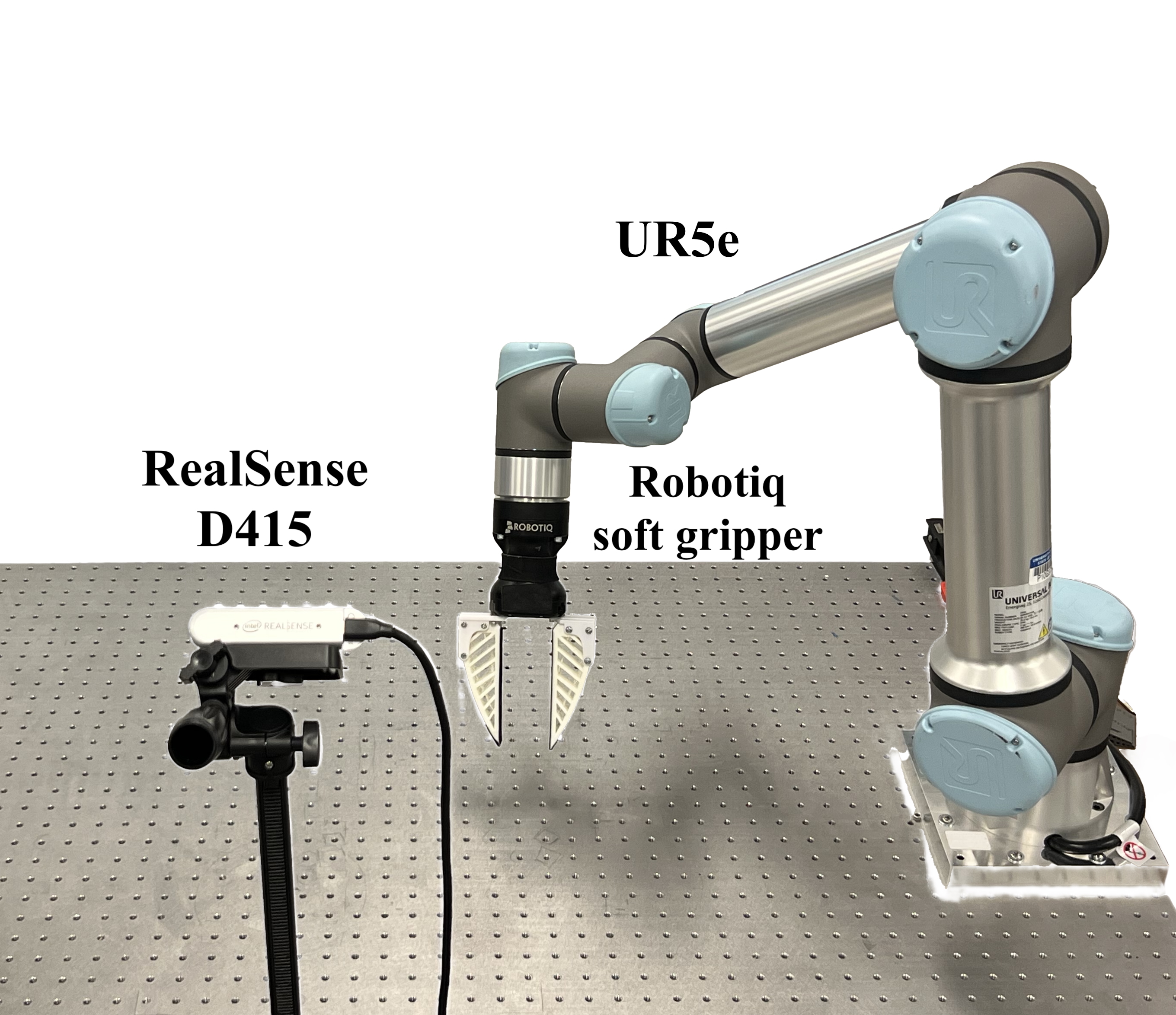
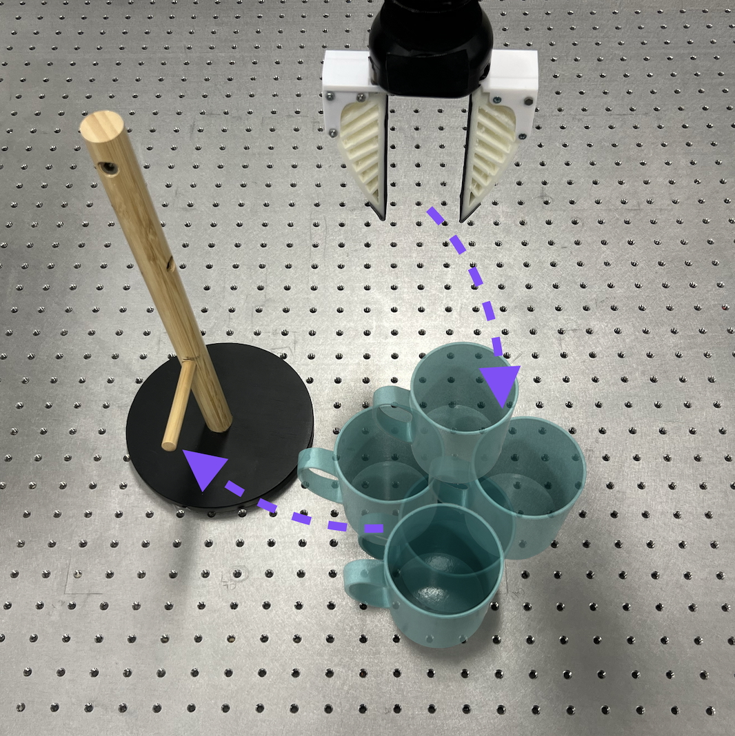
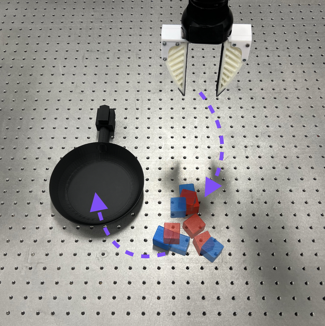
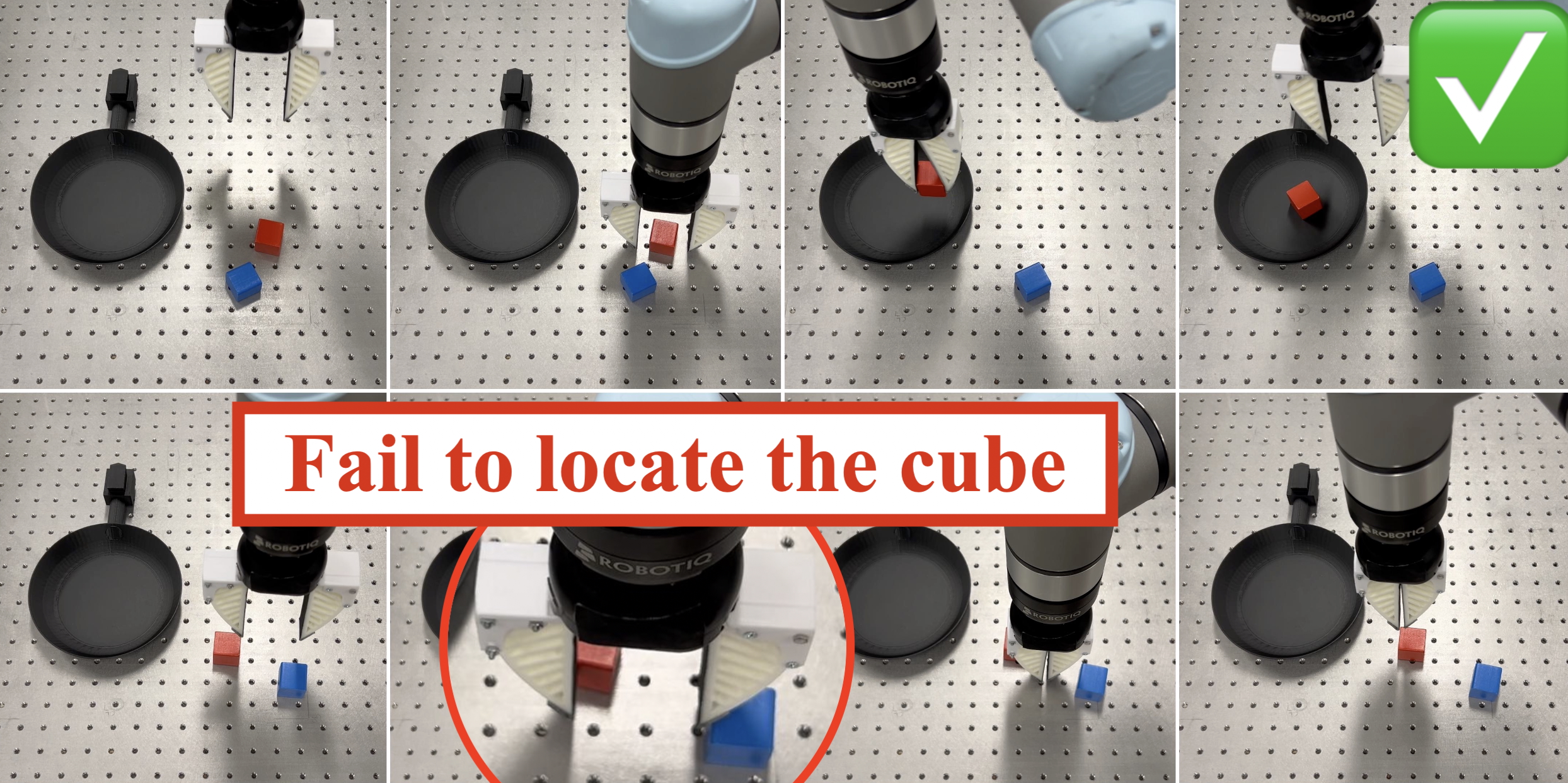
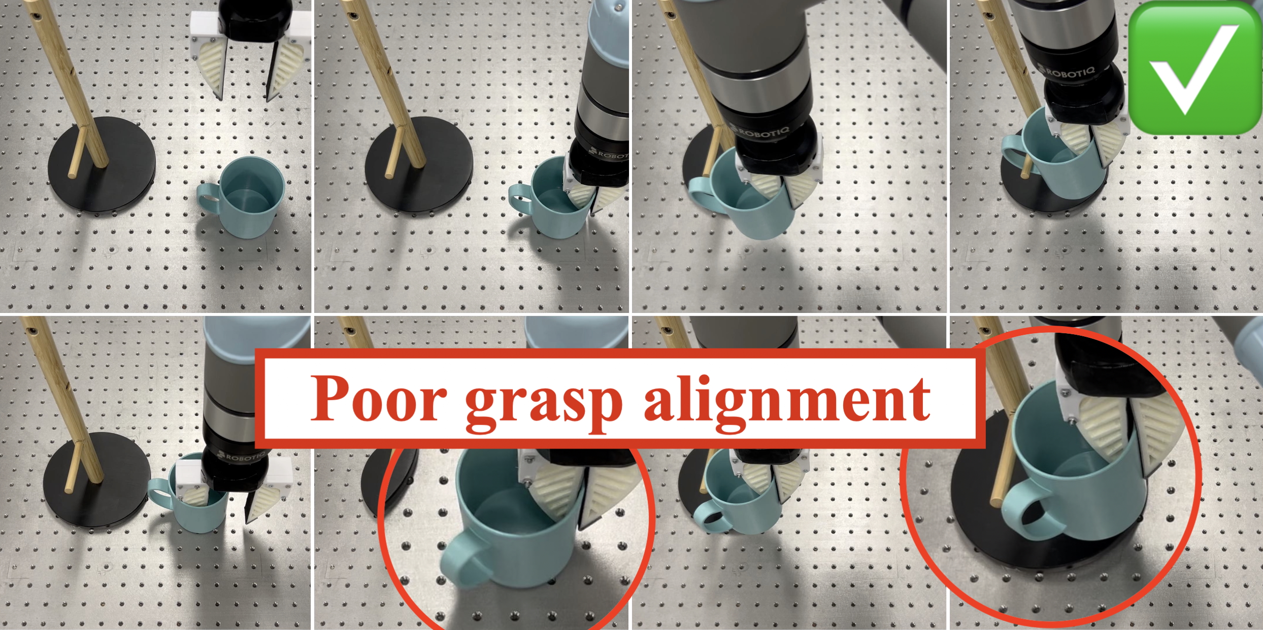
Simulation tasks come from MetaWorld, RLBench, and LIBERO. Physical tests use a UR5e arm, Robotiq gripper, and RealSense D415 camera for placing colored cubes into a bowl and hanging a mug at different heights. MetaWorld and RLBench goals are implicit in scenes; LIBERO and physical tasks use discrete task indices.
| MetaWorld | |||||||||
| Door | Drawer | Window | Peg | ||||||
| Policy | Open | Open | Assembly | Close | Insert | Hammer | Avg. | ||
| DP | 87.0 ± 1.92 | 100.0 ± 0.00 | 100.0 ± 0.00 | 94.0 ± 0.89 | 20.0 ± 1.22 | 24.0 ± 0.89 | 70.8 ± 0.24 | ||
| SDP | 80.0 ± 1.87 | 100.0 ± 0.00 | 100.0 ± 0.00 | 100.0 ± 0.00 | 20.5 ± 0.84 | 18.0 ± 1.64 | 69.8 ± 0.51 | ||
| MoDE | 100.0 ± 0.00 | 100.0 ± 0.00 | 94.0 ± 2.51 | 100.0 ± 0.00 | 19.5 ± 2.77 | 23.5 ± 0.89 | 72.8 ± 0.76 | ||
| FDP | 100.0 ± 0.00 | 100.0 ± 0.00 | 100.0 ± 0.00 | 100.0 ± 0.00 | 26.5 ± 2.19 | 22.0 ± 2.39 | 74.8 ± 0.67 | ||
| RLBench | |||||||||
| Close | Close | Close | Close | Toilet Seat | Take | Reach | Pick & | ||
| Policy | Box | Drawer | Fridge | Microwave | Down | Umbrella | Target | Lift | Avg. |
| DP | 33.5 ± 1.52 | 100.0 ± 0.00 | 77.0 ± 1.64 | 65.5 ± 1.48 | 64.0 ± 2.19 | 19.0 ± 1.95 | 3.5 ± 0.89 | 2.0 ± 0.84 | 45.6 ± 0.43 |
| SDP | 24.0 ± 1.34 | 100.0 ± 0.00 | 68.0 ± 3.11 | 42.5 ± 2.00 | 58.5 ± 2.88 | 6.5 ± 1.14 | 36.0 ± 2.61 | 1.0 ± 0.55 | 42.1 ± 0.70 |
| MoDE | 31.0 ± 2.88 | 97.0 ± 2.17 | 70.5 ± 1.64 | 50.5 ± 1.10 | 60.0 ± 1.73 | 10.5 ± 1.92 | 37.0 ± 1.10 | 3.5 ± 1.95 | 45.0 ± 0.87 |
| FDP | 72.0 ± 1.30 | 100.0 ± 0.00 | 75.5 ± 1.10 | 93.0 ± 1.92 | 27.5 ± 2.12 | 78.0 ± 2.17 | 61.0 ± 1.52 | 4.5 ± 2.39 | 63.9 ± 0.23 |
| MetaWorld | RLBench | ||||||||||
| Door | Drawer | Window | Open | Open | Open | Open | |||||
| Method | Policy | Close | Close | Disassemble | Open | Avg. | Box | Drawer | Fridge | Microwave | Avg. |
| Full Parameter | DP | 100.0 ± 0.00 | 100.0 ± 0.00 | 60.5 ± 1.10 | 100.0 ± 0.00 | 90.1 ± 0.27 | 75.5 ± 1.30 | 81.0 ± 0.55 | 64.0 ± 2.07 | 63.5 ± 1.52 | 71.0 ± 0.76 |
| SDP | 89.5 ± 2.05 | 100.0 ± 0.00 | 58.0 ± 2.17 | 100.0 ± 0.00 | 86.9 ± 0.31 | 67.0 ± 0.84 | 88.5 ± 2.88 | 58.5 ± 2.61 | 66.0 ± 1.52 | 70.0 ± 0.90 | |
| MoDE | 100.0 ± 0.00 | 100.0 ± 0.00 | 66.5 ± 2.97 | 100.0 ± 0.00 | 91.6 ± 0.74 | 60.5 ± 0.45 | 88.0 ± 1.92 | 71.0 ± 0.89 | 75.0 ± 1.22 | 73.6 ± 0.48 | |
| FDP | 100.0 ± 0.00 | 100.0 ± 0.00 | 62.0 ± 2.17 | 100.0 ± 0.00 | 90.5 ± 0.54 | 87.0 ± 1.92 | 72.5 ± 3.39 | 65.0 ± 1.87 | 79.0 ± 1.67 | 75.9 ± 0.91 | |
| Router | SDP | 72.0 ± 1.30 | 0.0 ± 0.00 | 1.0 ± 0.55 | 4.0 ± 1.52 | 19.3 ± 0.67 | 4.5 ± 1.92 | 23.5 ± 1.95 | 11.5 ± 1.14 | 15.5 ± 2.49 | 13.8 ± 0.40 |
| MoDE | 4.0 ± 2.30 | 1.0 ± 0.89 | 1.5 ± 1.34 | 24.0 ± 1.67 | 7.6 ± 1.08 | 2.5 ± 1.41 | 4.0 ± 1.95 | 19.5 ± 0.84 | 1.5 ± 1.34 | 6.9 ± 0.71 | |
| FDP | 85.5 ± 1.48 | 64.5 ± 2.28 | 4.0 ± 2.19 | 5.5 ± 0.84 | 39.9 ± 0.67 | 17.5 ± 1.41 | 1.5 ± 1.34 | 17.5 ± 1.73 | 0.0 ± 0.00 | 9.1 ± 0.82 | |
| + Observation Encoder | SDP | 100.0 ± 0.00 | 100.0 ± 0.00 | 31.0 ± 0.89 | 100.0 ± 0.00 | 82.8 ± 0.22 | 25.5 ± 0.84 | 48.0 ± 2.17 | 41.0 ± 1.14 | 22.5 ± 1.87 | 34.3 ± 0.45 |
| MoDE | 93.0 ± 0.45 | 100.0 ± 0.00 | 40.0 ± 1.58 | 100.0 ± 0.00 | 83.2 ± 0.37 | 19.0 ± 1.34 | 65.5 ± 1.10 | 29.5 ± 1.30 | 25.0 ± 1.00 | 34.8 ± 0.91 | |
| FDP | 100.0 ± 0.00 | 93.0 ± 2.68 | 52.5 ± 1.87 | 100.0 ± 0.00 | 86.4 ± 0.99 | 30.0 ± 3.08 | 57.0 ± 1.48 | 47.5 ± 2.55 | 18.5 ± 1.82 | 38.3 ± 1.19 | |
| + New Module | SDP | 100.0 ± 0.00 | 100.0 ± 0.00 | 60.5 ± 1.79 | 100.0 ± 0.00 | 90.1 ± 0.45 | 69.0 ± 1.14 | 23.5 ± 2.88 | 40.5 ± 1.92 | 22.5 ± 1.00 | 38.9 ± 0.89 |
| MoDE | 100.0 ± 0.00 | 100.0 ± 0.00 | 61.5 ± 2.30 | 100.0 ± 0.00 | 90.4 ± 0.58 | 58.0 ± 1.92 | 54.0 ± 1.14 | 58.0 ± 1.79 | 53.0 ± 1.92 | 55.8 ± 0.78 | |
| FDP | 100.0 ± 0.00 | 100.0 ± 0.00 | 68.5 ± 1.52 | 100.0 ± 0.00 | 92.1 ± 0.38 | 86.5 ± 1.34 | 77.0 ± 1.10 | 78.0 ± 2.28 | 77.5 ± 3.08 | 79.8 ± 0.91 | |
Implementations
Policies receive RGB images and joint angles, use two observations of history, predict 16 joint-angle steps, and execute eight before replanning. FDP uses four U-Net diffusion modules. Baselines follow their original designs, with MoDE reduced in size for comparison; new components copy existing weights.
Multitask Learning
The first comparison learns several tasks together from demonstrations.
1 Simulation
Training uses 25 demonstrations per task for six MetaWorld tasks and 50 for eight RLBench tasks. Evaluation reports 40 rollouts per task per seed across five seeds. Table I gives average success of 74.8% versus 70.8% for DP on MetaWorld and 63.9% versus 45.6% on RLBench. Improvements vary by task, with some baselines matching or exceeding FDP on individual tasks.
2 Real-world
Physical multitask training uses 300 red-cube and 200 low-mug demonstrations. Across 20 trials per task, FDP succeeds 15 and 17 times, compared with DP’s 14 and 16. These small trial counts show a modest advantage in this setup; selected rollouts illustrate baseline placement errors.
Task Transfer and Adaptation
Adaptation compares full fine-tuning with router-only tuning, encoder-plus-router tuning, and adding a new component. These partial FDP settings update approximately 0.5%, 11%, and 27% of parameters respectively.
| Method | Policy | Cube Blue | Hang High |
| Full Param. | DP | 15 / 20 | 17 / 20 |
| SDP | 14 / 20 | 16 / 20 | |
| MoDE | 15 / 20 | 16 / 20 | |
| FDP | 17 / 20 | 15 / 20 | |
| Router + Obs. Enc. | SDP | 10 / 20 | 9 / 20 |
| MoDE | 10 / 20 | 11 / 20 | |
| FDP | 11 / 20 | 11 / 20 | |
| + New Module | SDP | 13 / 20 | 11 / 20 |
| MoDE | 14 / 20 | 13 / 20 | |
| FDP | 17 / 20 | 17 / 20 |
1 Simulation
Four new tasks per simulation benchmark use ten demonstrations each in MetaWorld and 25 in RLBench. Evaluation uses 60 and 40 rollouts per seed respectively. Adding a component yields FDP averages of 92.1% and 79.8%, versus 90.5% and 75.9% with full fine-tuning. Router-only adaptation is often insufficient.
2 Real-world
Blue-cube and high-mug adaptation each use 100 demonstrations and 20 evaluation trials. Adding a component reaches 17/20 on both tasks. Full FDP fine-tuning reaches 17/20 and 15/20; full DP reaches 15/20 and 17/20. Modular adaptation therefore works well here without dominating every full-tuning result.
| # Comp | MetaWorld | RLBench |
| 2 | 86.7 ± 0.89 | 54.4 ± 1.22 |
| 3 | 90.0 ± 0.71 | 58.8 ± 0.84 |
| 4 | 91.3 ± 0.45 | 63.9 ± 0.23 |
| 5 | 91.3 ± 0.89 | 64.4 ± 0.71 |
| 6 | 91.7 ± 1.14 | 65.0 ± 0.45 |
| 7 | 91.9 ± 0.55 | 65.6 ± 0.84 |
Analysis
Further experiments examine capacity, data, inference cost, continual adaptation, retention, and the interpretation of components.
Scaling of Number of Diffusion Components
Increasing the component count from two to four improves the selected task sets, with diminishing gains beyond four. The authors find four to six components useful for these experiments. Computation grows approximately linearly with component count; pruning offers an explicit speed–performance trade-off.
| Policy | Close Box | Close Drawer | Close Fridge | Close Microwave | Toilet Seat Down | Take Umbrella | Reach Target | Pick & Lift | Avg. |
| DP | 33.5 ± 1.52 | 100.0 ± 0.00 | 77.0 ± 1.64 | 65.5 ± 1.48 | 64.0 ± 2.19 | 19.0 ± 1.95 | 3.5 ± 0.89 | 2.0 ± 0.84 | 45.6 ± 0.43 |
| FDP | 72.0 ± 1.30 | 100.0 ± 0.00 | 75.5 ± 1.10 | 93.0 ± 1.92 | 27.5 ± 2.12 | 78.0 ± 2.17 | 61.0 ± 1.52 | 4.5 ± 2.39 | 63.9 ± 0.23 |
| FDP | 63.5 ± 1.14 | 95.5 ± 1.64 | 69.0 ± 1.00 | 90.5 ± 0.71 | 22.5 ± 2.70 | 30.5 ± 2.70 | 41.5 ± 1.30 | 1.0 ± 0.55 | 51.8 ± 0.27 |
| Multitask 4 Experts | + Expert Modules (5–12) | |||||||||||||||||||||||||||||||||||||
| Policy |
|
|
|
|
|
|
|
|
|
|
|
|
| |||||||||||||||||||||||||
| SDP | 57.2 ± 1.56 | 22.4 ± 1.04 | 100.0 ± 0.00 | 50.8 ± 1.34 | 30.4 ± 0.67 | 56.0 ± 1.50 | 46.4 ± 0.88 | 94.8 ± 2.63 | 56.0 ± 1.13 | 22.4 ± 0.36 | 25.6 ± 1.73 | 35.6 ± 1.43 | 49.8 ± 0.44 | |||||||||||||||||||||||||
| MoDE | 65.2 ± 1.84 | 33.6 ± 0.36 | 94.8 ± 0.72 | 45.6 ± 1.91 | 30.8 ± 0.91 | 63.6 ± 0.67 | 41.6 ± 1.91 | 100.0 ± 0.00 | 58.8 ± 1.21 | 35.6 ± 1.54 | 42.4 ± 1.54 | 50.8 ± 1.21 | 55.2 ± 0.30 | |||||||||||||||||||||||||
| FDP | 83.2 ± 0.91 | 34.4 ± 1.54 | 100.0 ± 0.00 | 60.8 ± 2.30 | 40.0 ± 0.57 | 89.6 ± 0.88 | 56.8 ± 1.75 | 100.0 ± 0.00 | 82.0 ± 1.26 | 40.8 ± 2.50 | 64.8 ± 1.21 | 55.6 ± 1.54 | 67.3 ± 0.39 | |||||||||||||||||||||||||
Scaling of Number of Tasks
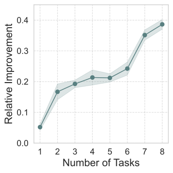
On the selected RLBench task combinations, FDP’s relative advantage over DP grows as more tasks are included. This supports its intended use for varied task distributions within the tested range.
Scaling of Number of Demonstrations
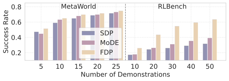
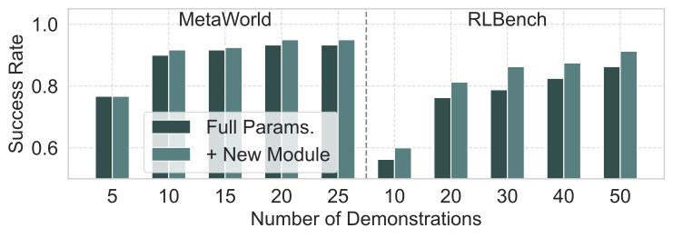
The data-scaling plots distinguish joint learning from adaptation.
1 Multitask Learning
More demonstrations generally improve multitask success. The reported comparisons favor FDP, particularly on the tested RLBench tasks; this is an empirical scaling observation rather than a universal sample-complexity guarantee.
2 Task Adaptation
Both full fine-tuning and adding a component improve with more adaptation data. On the selected RLBench tasks, component expansion can match or improve full tuning with fewer demonstrations.
Partial Reconstruction of Action Distribution
Keeping only the two highest-weight components at inference reduces mean RLBench success from 63.9% to 51.8%, a roughly 19% relative decrease. Table VI reports a twofold inference speedup without retraining. The table values and caption support 19%; the accompanying source prose says 17%.
Continual Adaptation
A LIBERO sequence starts with four components and four tasks, then adds one component for each of eight new tasks, ending with twelve. Across five seeds and 50 evaluations per seed, the reported overall average is 67.3% for FDP, 55.2% for MoDE, and 49.8% for SDP.
Knowledge Retention
The separate retention experiment reports 57.6% on four base tasks before adaptation, 29.3% after adaptation without replay, and 53.5% with five replay demonstrations per base task. These results show that frozen experts alone do not prevent forgetting. Frozen visual features and cached routers are suggested remedies; replay is the tested intervention.
| Policy |
|
|
|
|
| |||||||||
| FDP | 57.2 ± 1.56 | 22.4 ± 1.04 | 100.0 ± 0.00 | 50.8 ± 1.34 | 57.6 ± 0.61 | |||||||||
| FDP | 32.5 ± 1.00 | 5.0 ± 1.22 | 50.5 ± 1.10 | 29.0 ± 1.14 | 29.3 ± 0.45 | |||||||||
| FDP | 53.0 ± 1.64 | 17.5 ± 1.00 | 96.0 ± 0.89 | 47.5 ± 1.22 | 53.5 ± 0.63 |
Diffusion Components Analysis
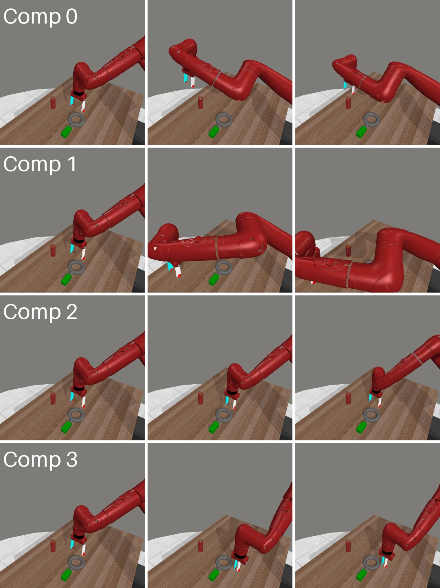
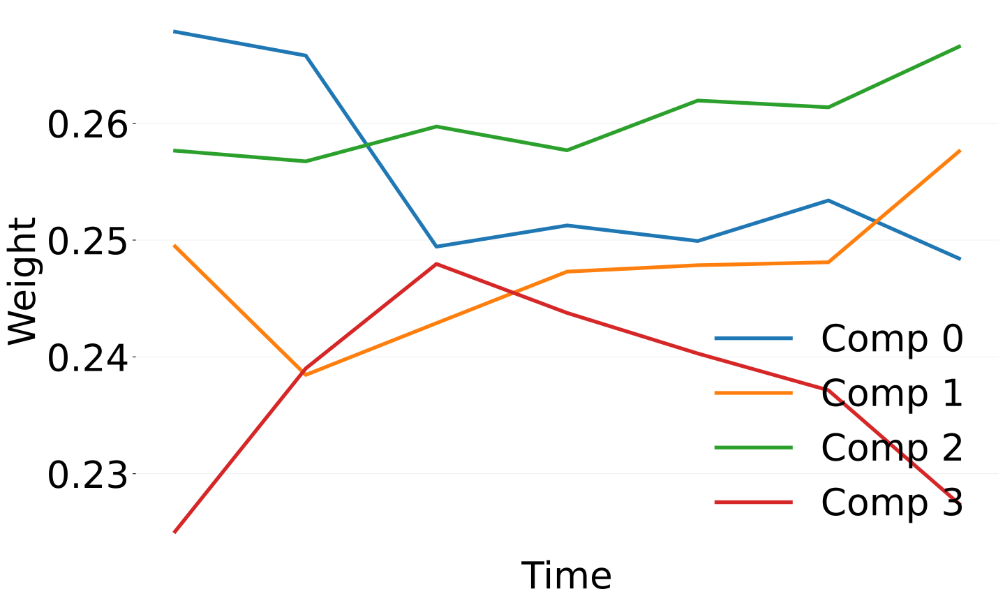
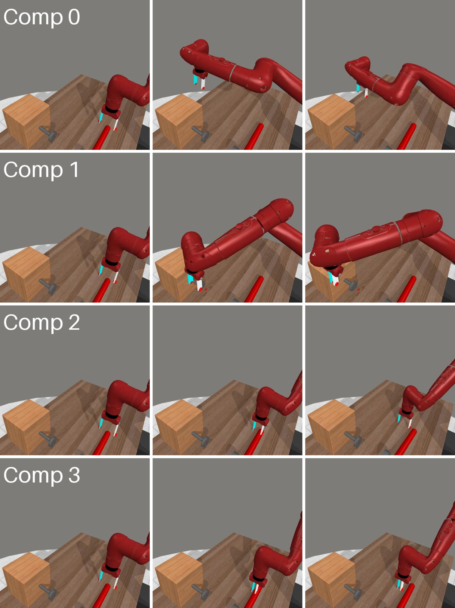
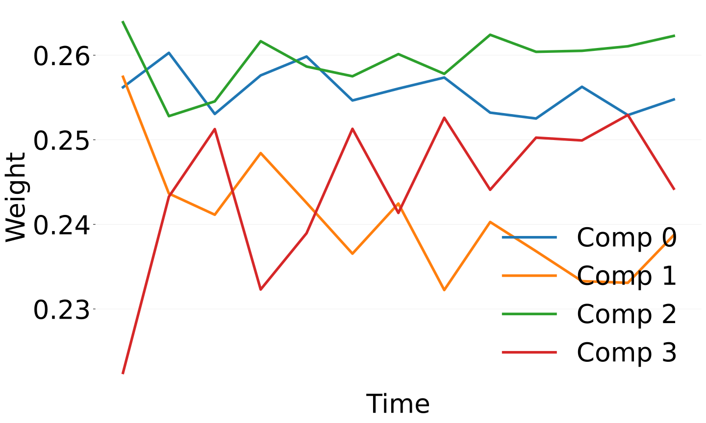
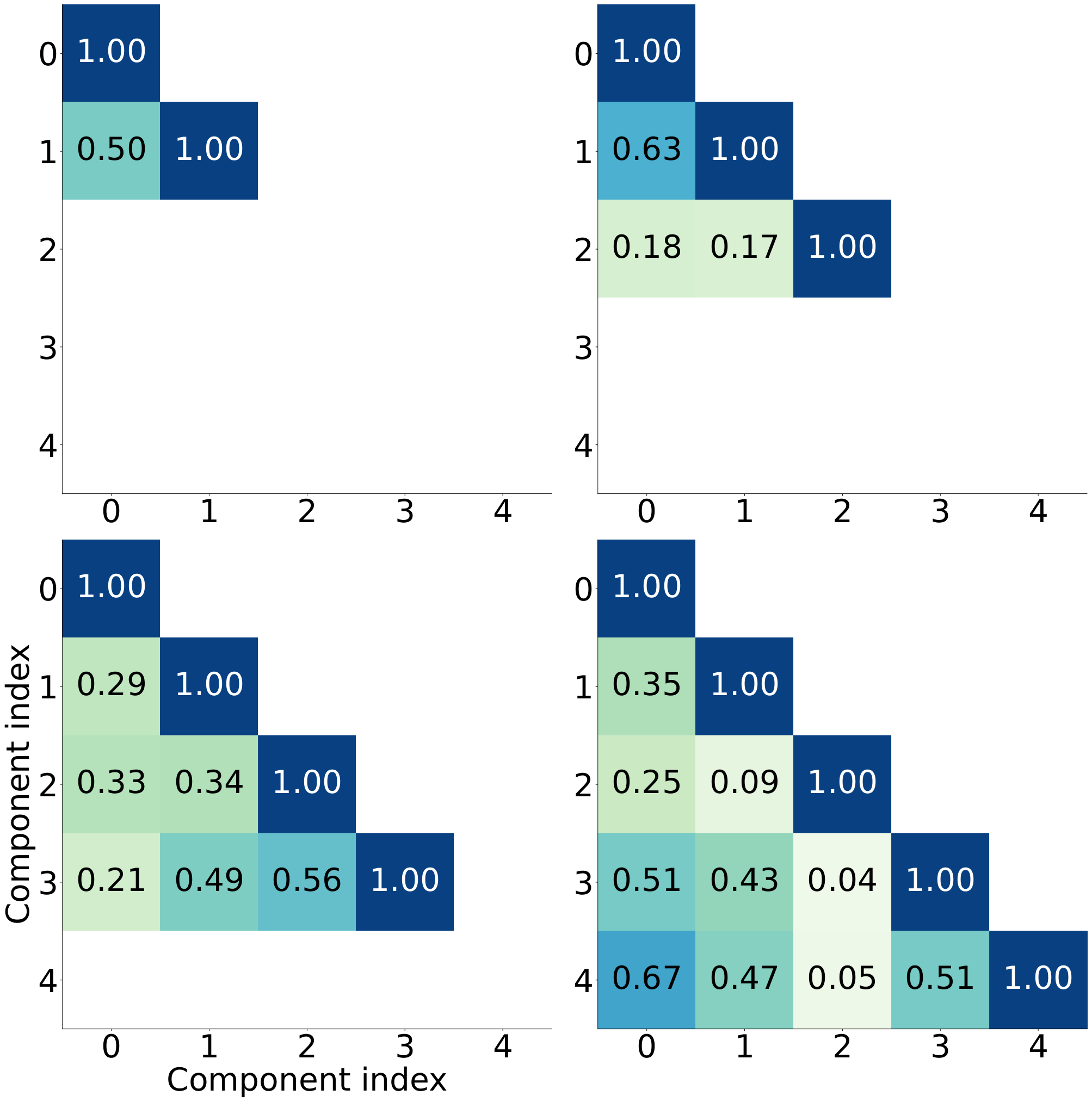
Assembly and hammer rollouts associate components with approach, alignment, and grasping phases. Pairwise score similarities show distinct but overlapping behavior, rather than orthogonal components. These observations suggest specialization but do not isolate causal roles through component removal. The source uses “Fig. 5” for both the demonstration-scaling and rollout panels; both panels are preserved.
Training Convergence of Policies
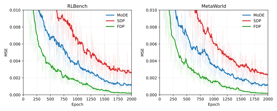
Validation denoising losses decrease faster and more steadily for FDP than the tested SDP and MoDE implementations. This measures optimization behavior on the reported datasets, separately from deployment success or wall-clock efficiency.
Conclusion And Limitations
Continuous composition of diffusion components improves several multitask and adaptation comparisons while supporting selective expansion. Current modules share architecture and size, specialization is primarily analyzed through visualizations, and retention still benefits from replay. Heterogeneous modules, component-removal studies, and longer continual-learning sequences remain future work.