Overview
QuantiPhy tests numerical physical inference from short videos: use a supplied size, speed, or acceleration to estimate another quantity. The contribution is a benchmark and diagnostic study, not a trained physical-reasoning model. All original figures, tables, displayed equations, and annotation-code examples are retained here, including the supplementary material.
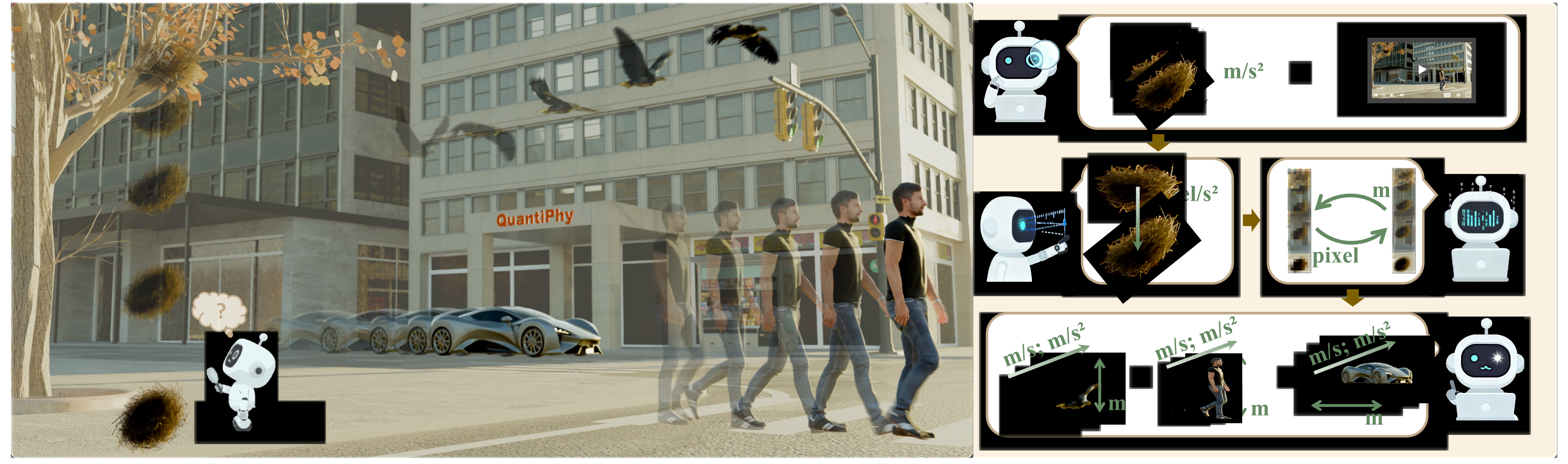
At a glance
The benchmark contains 569 videos and 3,355 questions spanning planar and three-dimensional motion with static or dynamic priors. Twenty-one vision-language models show substantial numerical errors. Video removal, counterfactual priors, and structured prompting reveal weak dependence on the intended evidence in many settings. These behavioral tests support concerns about input faithfulness, but do not directly establish whether an internal computation is memorization or reasoning.
1 Introduction
Qualitative physical question answering can hide large numerical mistakes: a nearly correct length and a tenfold error may both count as wrong. QuantiPhy instead scores positive numerical estimates of size, velocity, and acceleration. It complements physical-understanding benchmarks such as PhysBench and spatial evaluations such as VSI-Bench, adding explicit physical priors and controlled video diagnostics. Its applications to robotics or video realism are motivations rather than evaluated downstream results.
2 Related Work
The related work distinguishes qualitative physical benchmarks, multimodal or embodied reasoning systems, and conventional visual measurement. The proposed evaluation emphasizes quantitative kinematics and reliance on supplied evidence.
2.1 Benchmarks for VLM Physical Understanding
Earlier datasets cover collisions, support, material properties, scene relationships, and physical prediction, usually through classification or question answering. Spatial benchmarks add numerical distances and sizes, but generally emphasize static geometry. QuantiPhy focuses on time-dependent quantities inferred from moving objects and a specified physical reference.
2.2 Physical Reasoning Models
Strong language and video-generation models still make basic physical errors, and embodied agents can succeed on qualitative tasks without precise dynamics estimates. These results motivate a numerical evaluation; they do not imply that the benchmark exhausts physical reasoning or measures general motor competence.
2.3 Physical Understanding and Reasoning
Optical flow, detection, and tracking provide direct visual measurements, while human studies suggest use of relational cues and prior knowledge. QuantiPhy asks whether general vision-language models can combine these sources end to end. Accurate conventional measurement pipelines provide an existence argument for the task, rather than a baseline implemented in the reported comparison.
3 Methods
The method defines a single-prior inference task, constructs videos from several sources, and attaches numerical ground truth. Fixed cameras and controlled geometry make the intended pixel-to-world relation explicit.
3.1 Overview of QuantiPhy
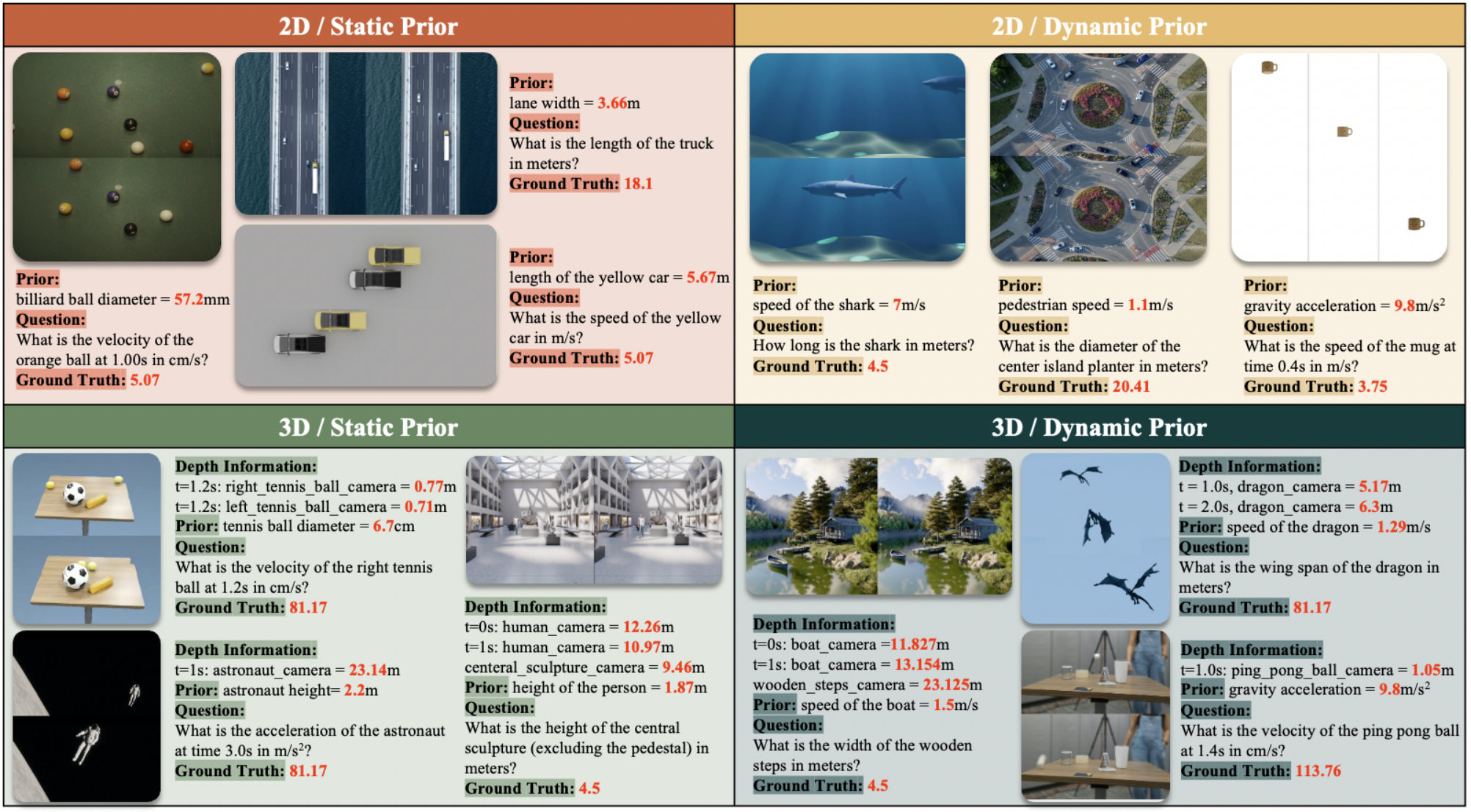
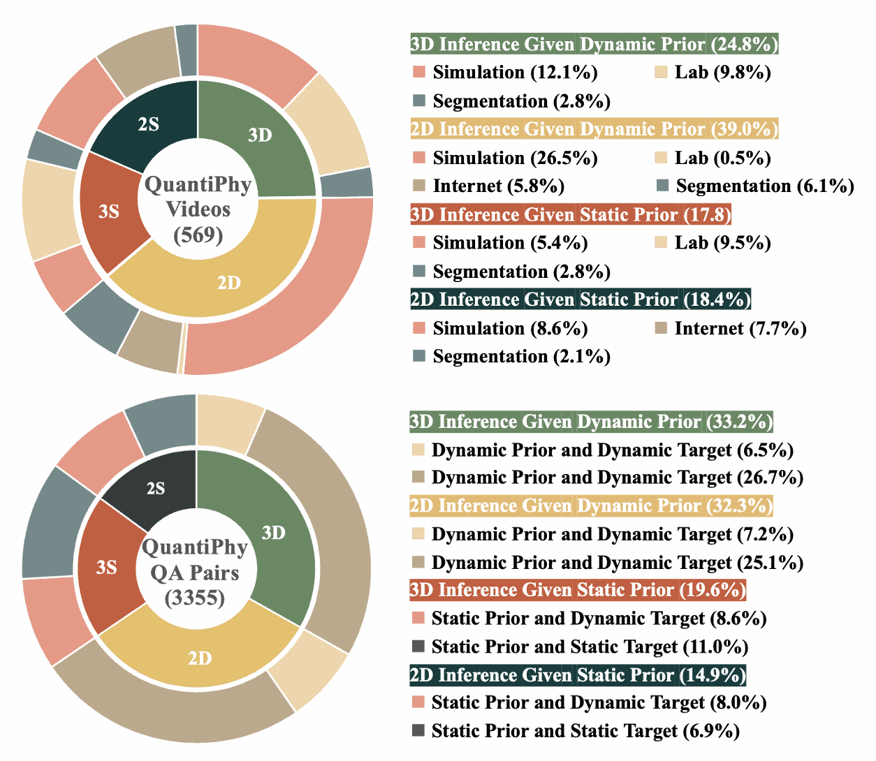
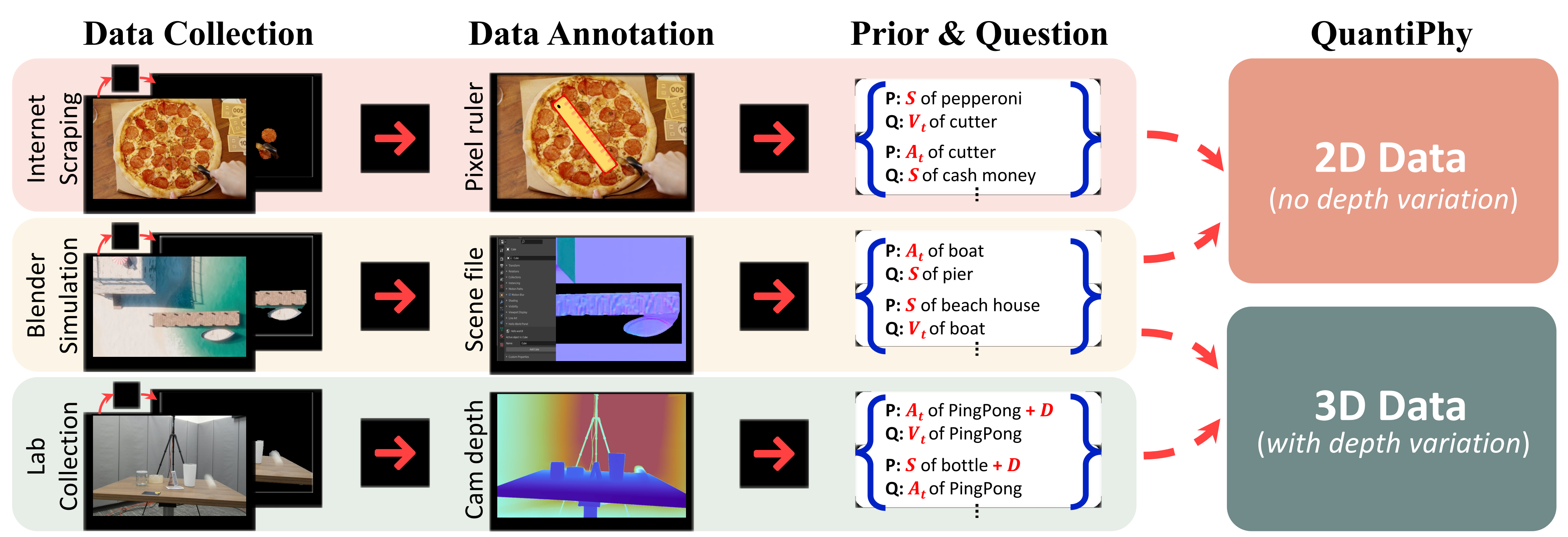
A question supplies one source object’s world-space size, velocity, or acceleration and requests a target quantity, possibly for another object. Pixel trajectories give finite-difference velocity and acceleration. Under planar geometry, the known prior calibrates one length-per-pixel scale, which transfers to other kinematic measurements. Three-dimensional cases add depth information. The four headline groups cross 2D/3D geometry with static/dynamic priors; the abbreviations 2S, 2D, 3S, and 3D refer to those groups. Rotation is outside the intended task.
Equation
3.2 Benchmark Construction
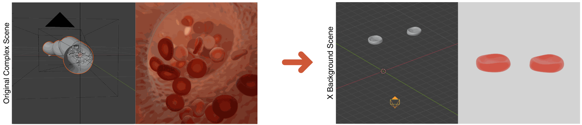
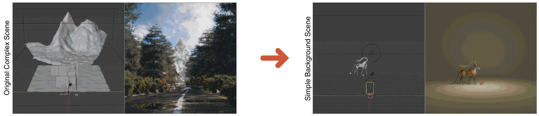
Data combine Blender scenes, calibrated lab recordings, and selected Internet or phone videos. Simulator quantities come from scene state; lab labels use calibrated geometry and measured depth; Internet labels use pixel rulers and approximate physical references. Segmentation creates background variants with unchanged annotations. Table 4 counts 300 Blender, 112 captured, 72 Internet, and 85 segmented clips, totaling 569; thus the main text’s claim that segmentation doubles the dataset does not match the reported final inventory. The prompts request a numerical answer with units.
4 Evaluation on QuantiPhy
The evaluation reports numerical accuracy across four task groups and compares model families, a sampled human survey, and targeted input perturbations. Provider settings and output parsing are part of the measurement pipeline.
4.1 Evaluation Setup
Twenty-one models comprise six proprietary and fifteen open models. Temperature is generally 0–0.1, but hosted defaults and output budgets differ: OpenAI models receive up to 10,000 tokens versus roughly 500–2,048 for open models. Mean Relative Accuracy averages ten binary relative-error tolerances, then averages category scores equally. The main text uses confidence thresholds {0.1, 0.2, …, 0.9, 0.95}, whereas Appendix A.2 uses {0.5, 0.55, …, 0.95}; these are materially different metrics. The main text averages valid numeric answers only, while Appendix A.3 assigns failures zero. Up to five identical-prompt attempts seek the first parseable answer. These reporting inconsistencies should be resolved before reproducing the scores.
Equation
4.2 Main Results
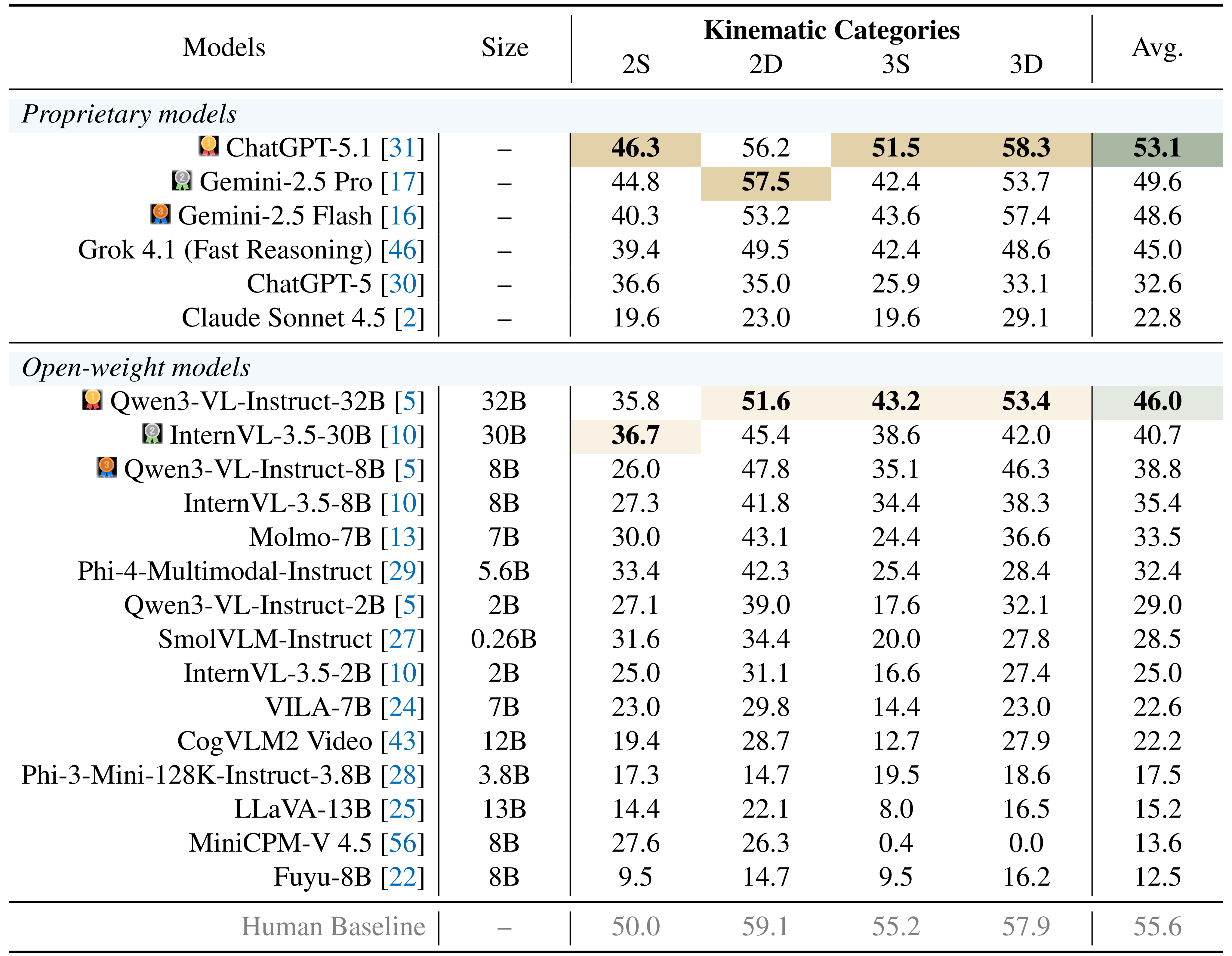
Table 1 reports human mean 55.6%, GPT-5.1 53.1%, Gemini 2.5 Pro 49.6%, GPT-5 32.6%, and Claude Sonnet 4.5 22.8%. Qwen3-VL-32B leads the open models at 46.0%; InternVL-30B reaches 40.7%. Within Qwen, scores rise from 29.0 at 2B to 38.8 at 8B and 46.0 at 32B, consistent with a scale benefit without isolating its cause. Human results come from sampled survey questions and different viewing tools, so this is not a matched full-benchmark comparison. Humans are also not a theoretical ceiling: exact measurements could outperform visual estimation under the benchmark assumptions.
5 Dissecting Quantitative Reasoning in VLMs
The diagnostics examine scene context, video dependence, sensitivity to counterfactual priors, and a prescribed measurement chain. The last three experiments use a 161-instance, 2D-only subset, whose scores should not be compared directly with full-benchmark averages.
5.1 Effect of Scene Context
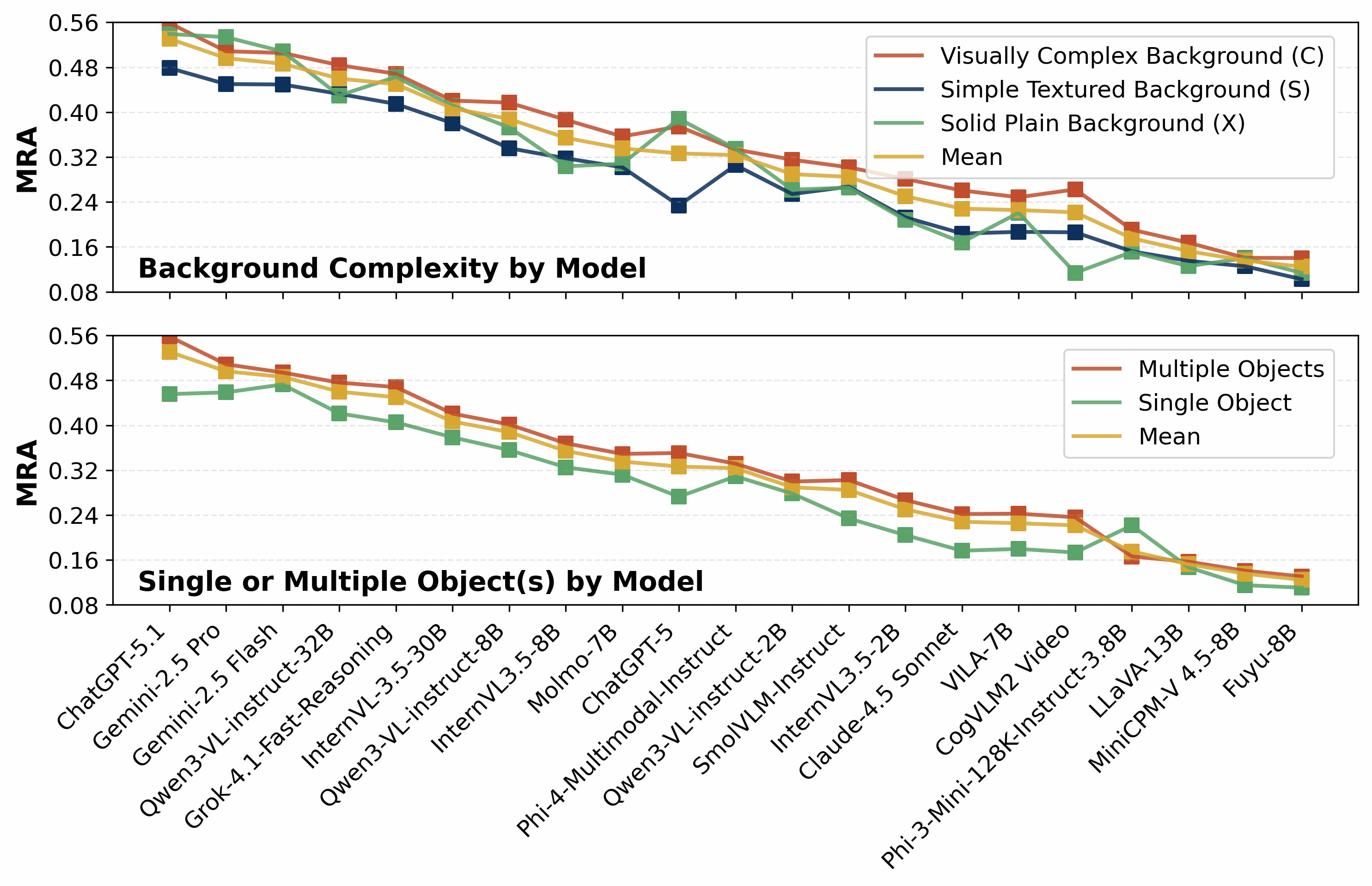
Complex scenes and questions requiring multiple objects often score better than simpler or single-object conditions. Possible explanations include familiar scale cues and relational references. The categories are not wholly paired interventions: some scenes are reused and others are unique, and the single/multiple label counts objects needed for the question, not everything visible. These aggregate differences therefore do not isolate a causal benefit from clutter or additional objects.
5.2 Do VLMs Use Videos and Priors Faithfully?
The analysis removes videos while retaining text, then separately rescales the supplied physical prior while keeping the video fixed. These probe reliance on visual evidence and numerical conditioning rather than train a better model.
Key finding: VLMs rely more on learned prior knowledge than visual inputs for physical reasoning.
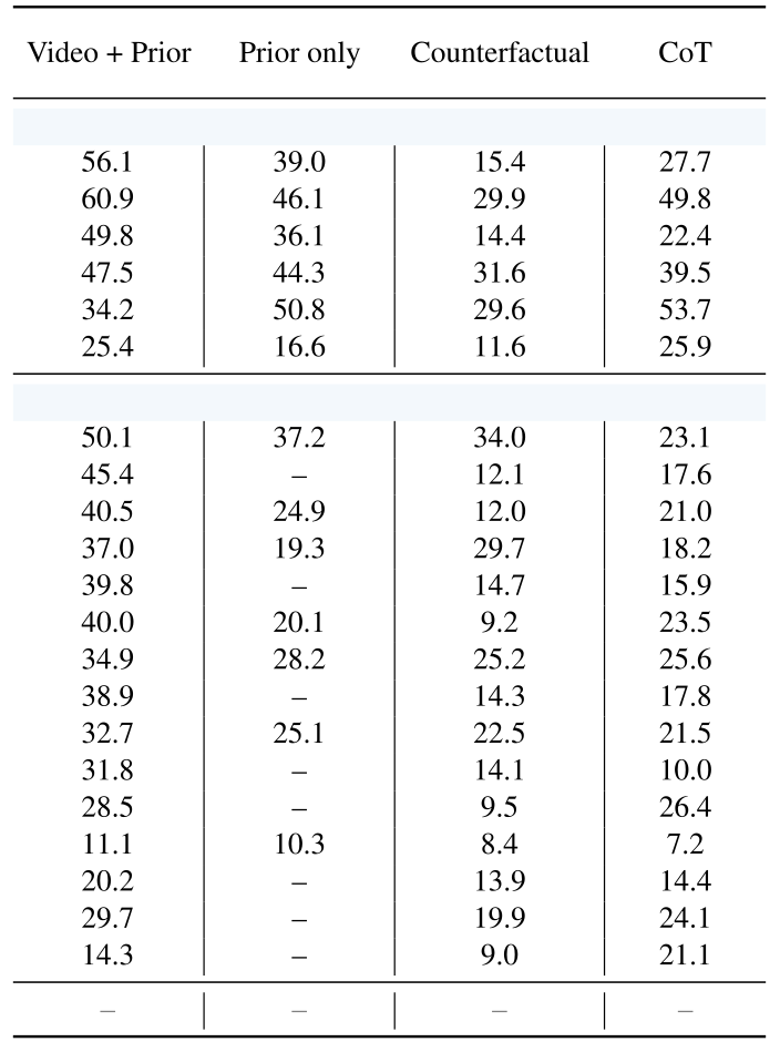
Prior-only scores can remain surprisingly strong on the subset; GPT-5 even scores higher without the video in Table 2. Other systems show appreciable drops, and several entries are unavailable. The results support substantial predictive information in object descriptions and familiar physical magnitudes, but neither small changes nor model-specific reversals prove that all visual information is ignored.
Key finding: VLMs (mostly) do not reason but memorize.
The counterfactual test multiplies the prior by one of ten factors from 0.001 to 700 and scales the expected answer accordingly. Many scores deteriorate sharply, consistent with weak obedience to the supplied numerical reference. The table also has exceptions: for GPT-5, 34.2 becomes 29.6, far smaller than the prose’s generalized 70–80% drops. Failure under these unusual priors establishes a behavioral limitation; it does not distinguish memorization from mistaken geometry, units, or inference.
5.3 Do Structured Prompts Help VLMs Reason?
The structured prompt asks sequentially for the source’s pixel quantity, pixel-to-world scale, target pixel quantity, and final world quantity. Parseable intermediate answers are appended to the context; failed steps are omitted. Table 2 shows improvements for GPT-5, Claude, and Fuyu, with decreases for the other eighteen models. The text’s “remaining 19” is an arithmetic inconsistency. Explicit decomposition can propagate erroneous measurements, so this particular four-step protocol is not a general test of every chain-of-thought strategy.
6 Discussion and Future Work
The results identify unreliable numerical grounding and sensitivity to prompts or supplied priors. The benchmark uses fixed cameras, mostly isolated translational motions, and simplified geometry; rotation, moving viewpoints, and complex interactions remain future work. Although the discussion calls objects rigid, the appendix permits articulated people or animals with a stable positional anchor. Physics-rich training and broader evaluations are proposals, not demonstrated remedies.
Acknowledgment
The authors acknowledge assistance with lab capture and support from NIH, Stanford HAI, Stanford graduate funding, and UST.
Appendix A More Studies and Results
The supplementary studies present selected model traces, explain the metric, and show score distributions. They add useful diagnostics while exposing differences in the documented scoring conventions.
A.1 Additional Case Studies
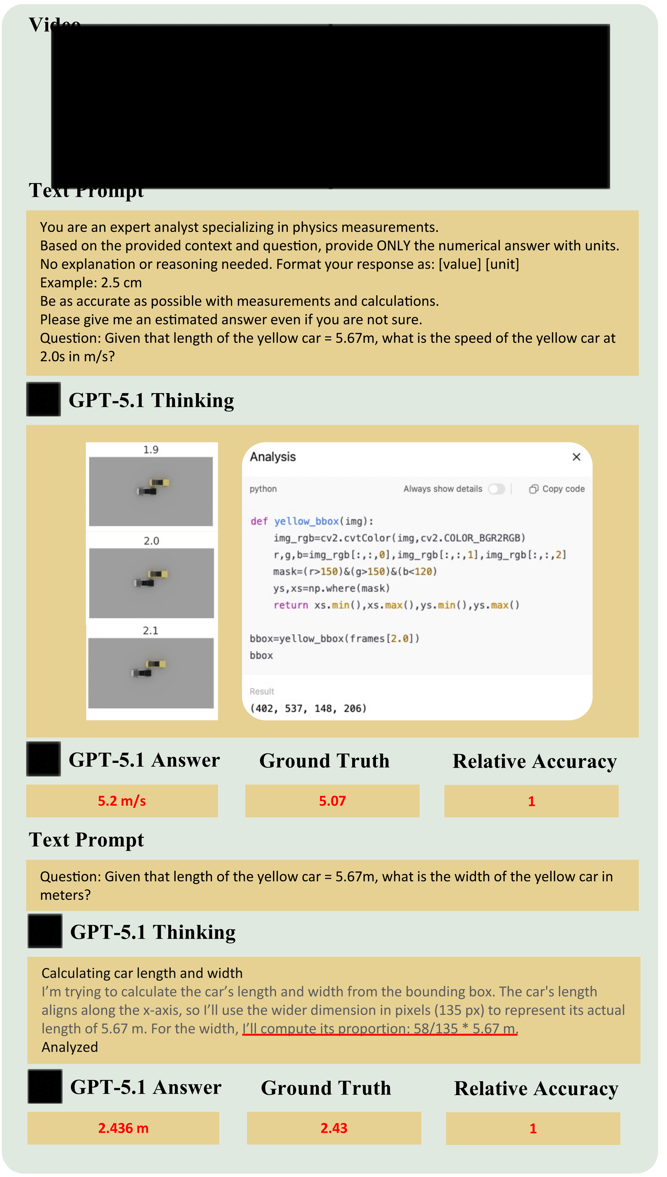
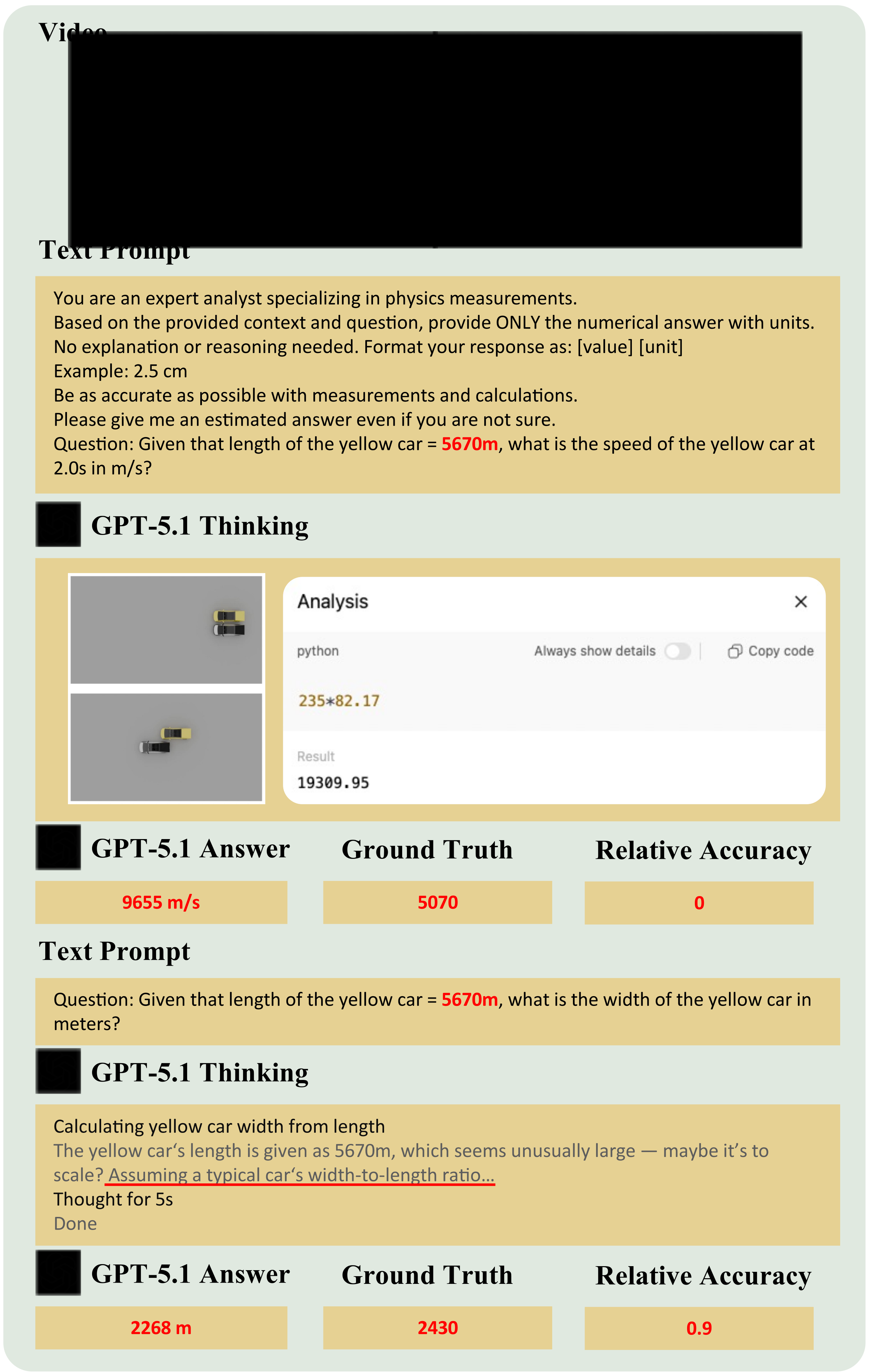
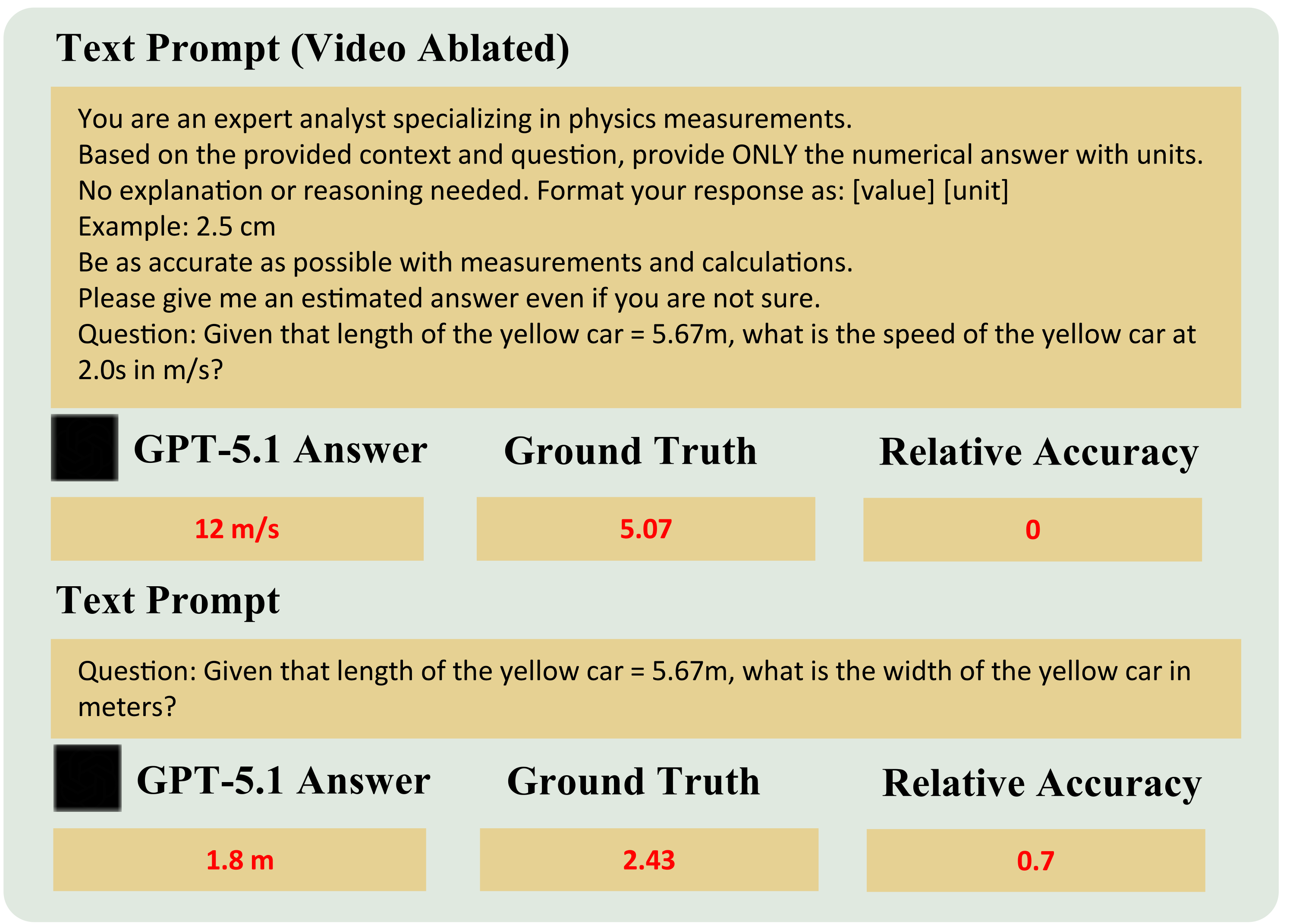
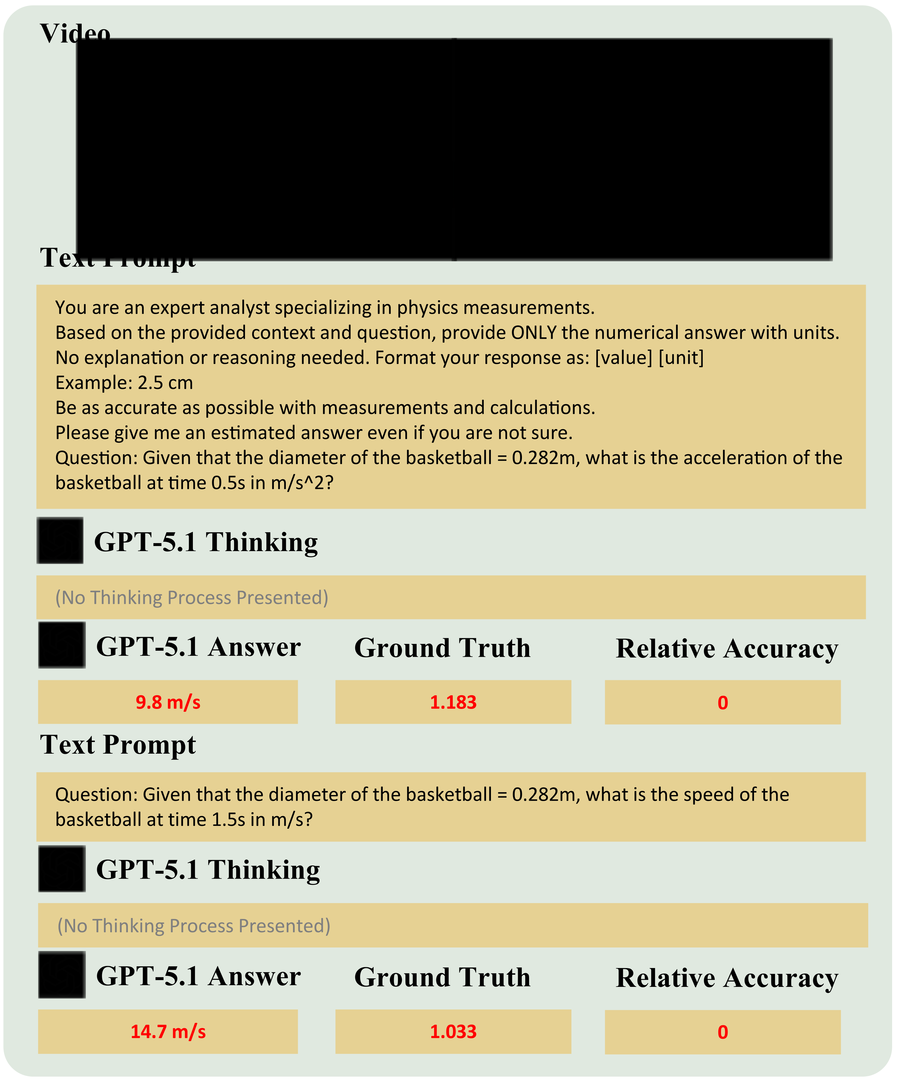
Four GPT-5.1 Thinking examples were selected manually after repeated queries in a tool-enabled user interface, so they are illustrative rather than an unbiased error sample or the main API protocol. A faithful car example measures pixels and predicts width about 2.44 m. Under a 1,000-fold length prior, the model substitutes familiar car proportions for reliable measurement; this factor differs from the main test’s factor set. Without video, it guesses speed poorly but obtains a plausible width. A simulated basketball with nonstandard acceleration elicits Earth-gravity answers. Accurate final numbers can therefore coexist with an unsupported route to the answer; the selected traces do not quantify how often each mechanism occurs.
Equation
A.2 Metric Design Justification
MRA awards one point at each relative-error tolerance and averages them. The authors prefer partial credit to exact matching because temporal aliasing, blur, uncertain boundaries, and imperfect real-world references create measurement noise. The appendix’s confidence set {0.5, 0.55, …, 0.95} differs from Section 4.1’s set and is retained without silently choosing one. Its normalization assumes the positive, nonzero ground-truth values specified by the data schema.
Equation 1
| (1) |
A.3 Model MRA Distribution
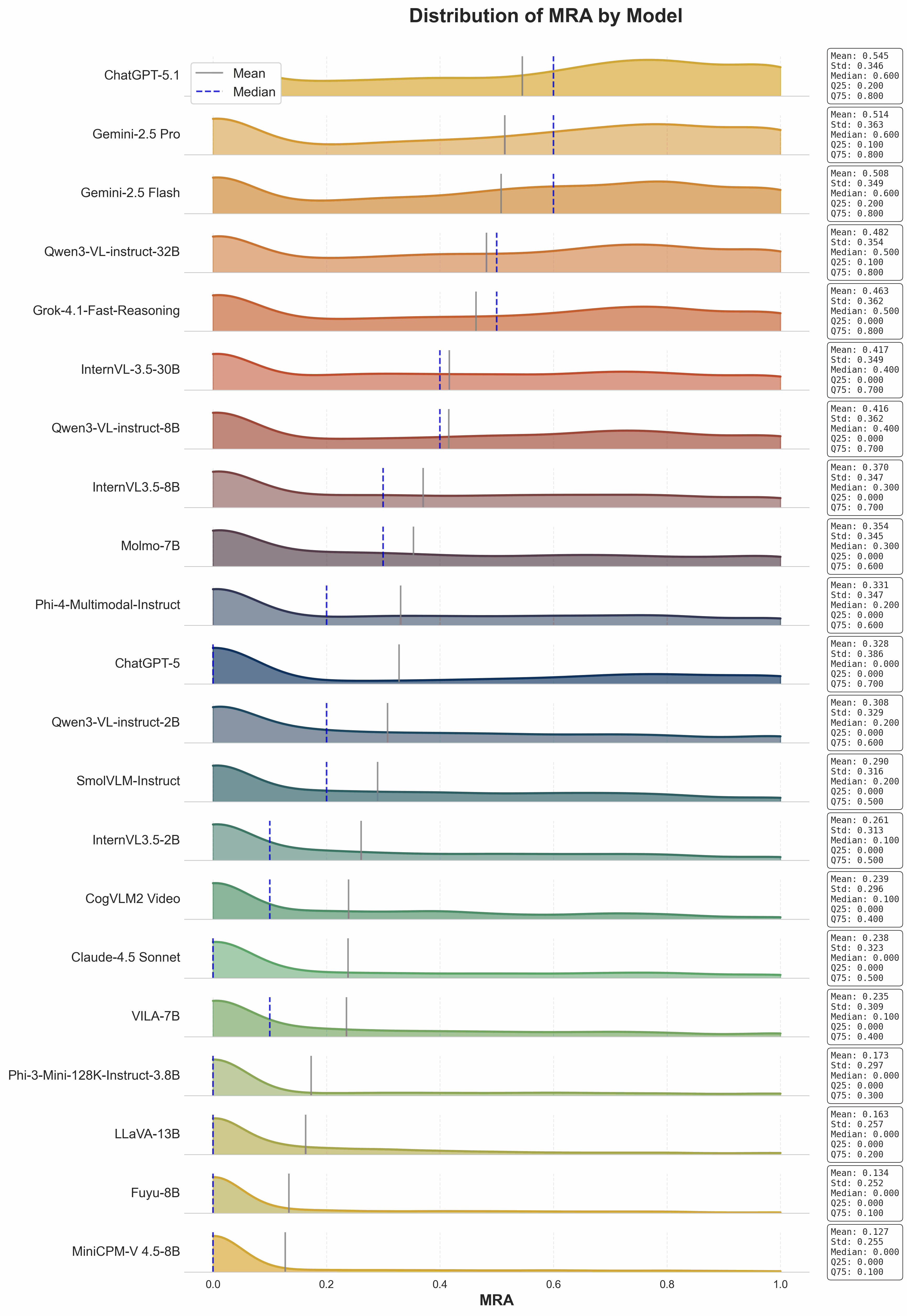
Figure 10 shows question-level density curves, means, medians, and quartiles. These means differ from Table 1’s equally weighted category averages. Stronger systems have more mass at moderate or high scores; weaker systems cluster near zero. Zero MRA can arise from a sufficiently inaccurate valid answer as well as zero output or parsing failure. This appendix explicitly treats API and other failures as zero, in tension with the main text’s valid-answer-only averaging.
Appendix B Dataset Construction Guidelines
The construction guidelines specify admissible videos, record fields, and a 36-code taxonomy. They explain which physical assumptions make a single reference sufficient.
B.1 General Principles
Clips should have a stationary camera and predominantly translational motion. Planar tasks constrain reference and target geometry to a common depth layer. “Rigid” is relaxed to include articulated entities whose motion has a stable center. Each record stores an identifier, source, four-character type, frame rate, prior/posterior type, question, positive physical prior, optional metric depth information, and positive numeric target. Units and instantaneous versus interval quantities must be explicit. These are construction requirements, with source-dependent measurement accuracy rather than a guarantee of exact real-world ground truth.
| Property | Example value |
|---|---|
| video_id | simulation_0032 |
| video_source | simulation |
| video_type | A3MC |
| fps | 30 |
| inference_type | DD |
| question | What is the acceleration of the orange car at 1.0s in m/s2? |
| ground_truth_prior | gravity acc = 9.8 m/s2 |
| depth_info | t=1s, distance_ball_camera = 13.80 m; |
| t=2s, distance_ball_camera = 13.80 m; | |
| t=1.5s, distance_orange_camera = 10.18 m; | |
| t=2s, distance_orange_camera = 10.40 m; | |
| t=2.5s, distance_green_camera = 4.32 m; | |
| t=3s, distance_green_camera = 6.91 m | |
| ground_truth_posterior | 2.86 |
B.2 Video Types
Each video receives a code describing its reference quantity, dimensionality, relevant-object count, and background. The benchmark tries to cover every combination with at least four examples.
B.2.1 Video Categories Definition
The first character is S/V/A for size, velocity, or acceleration prior. The second distinguishes planar 2D from 3D; the third is S/M for one versus multiple objects needed to answer the question. The final X/S/C denotes plain, simple, or complex background. Background complexity is a qualitative design choice, and irrelevant visible objects do not necessarily change the S/M label. Figures 11–14 illustrate these distinctions.
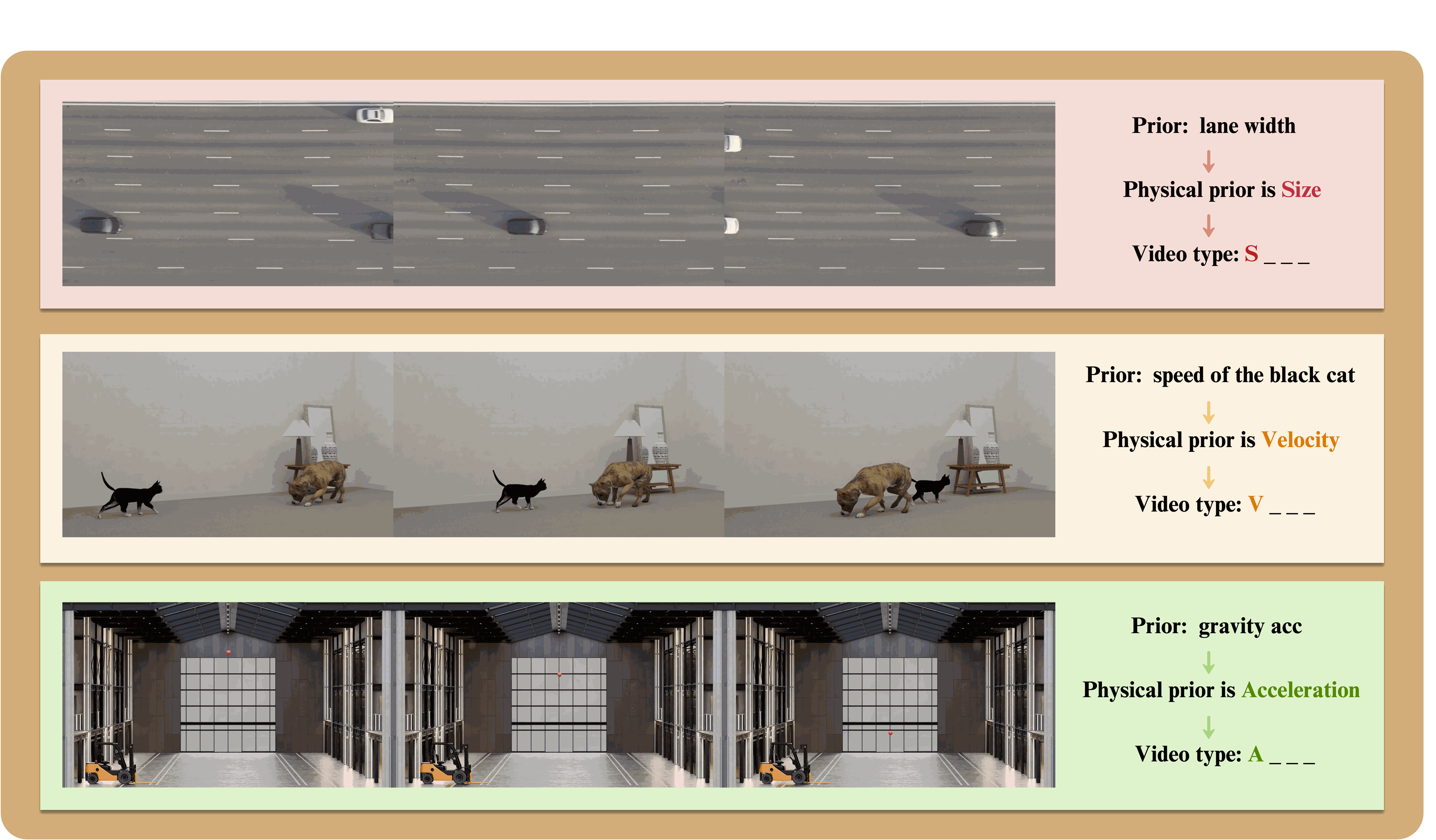
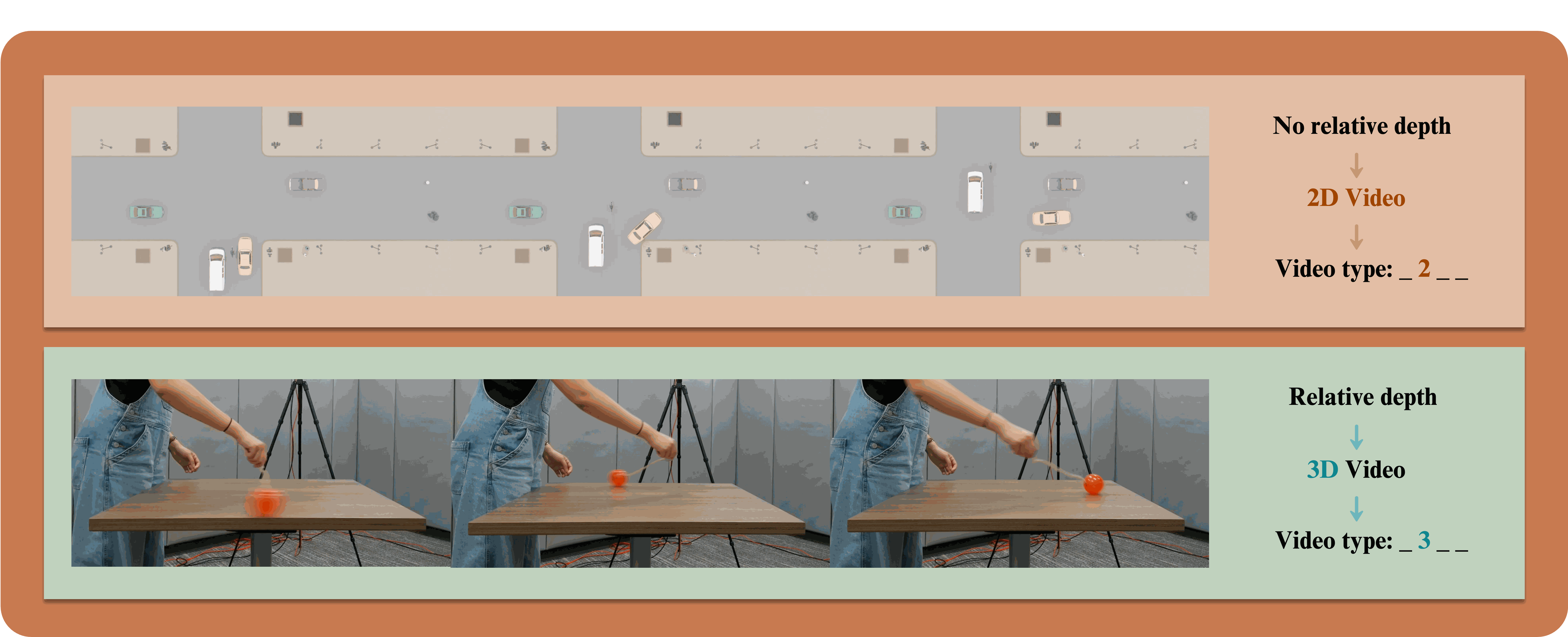
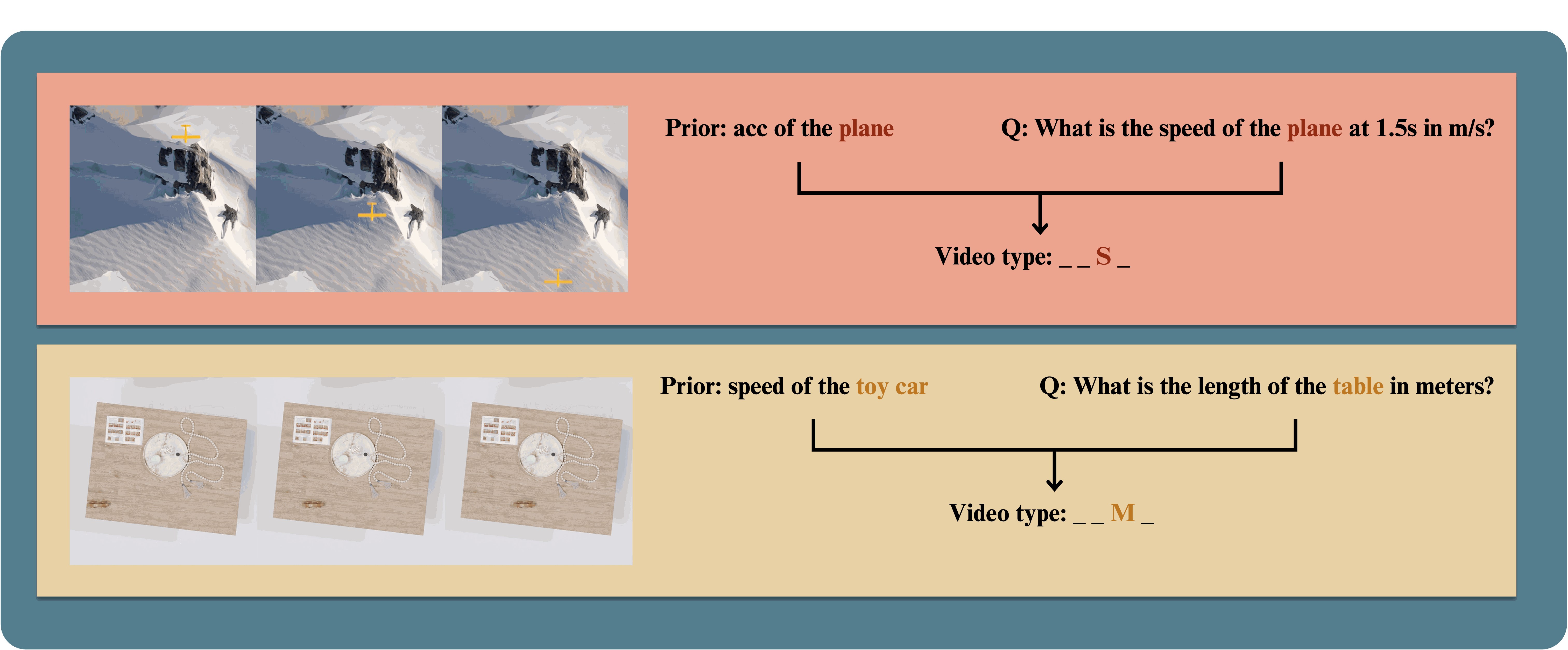
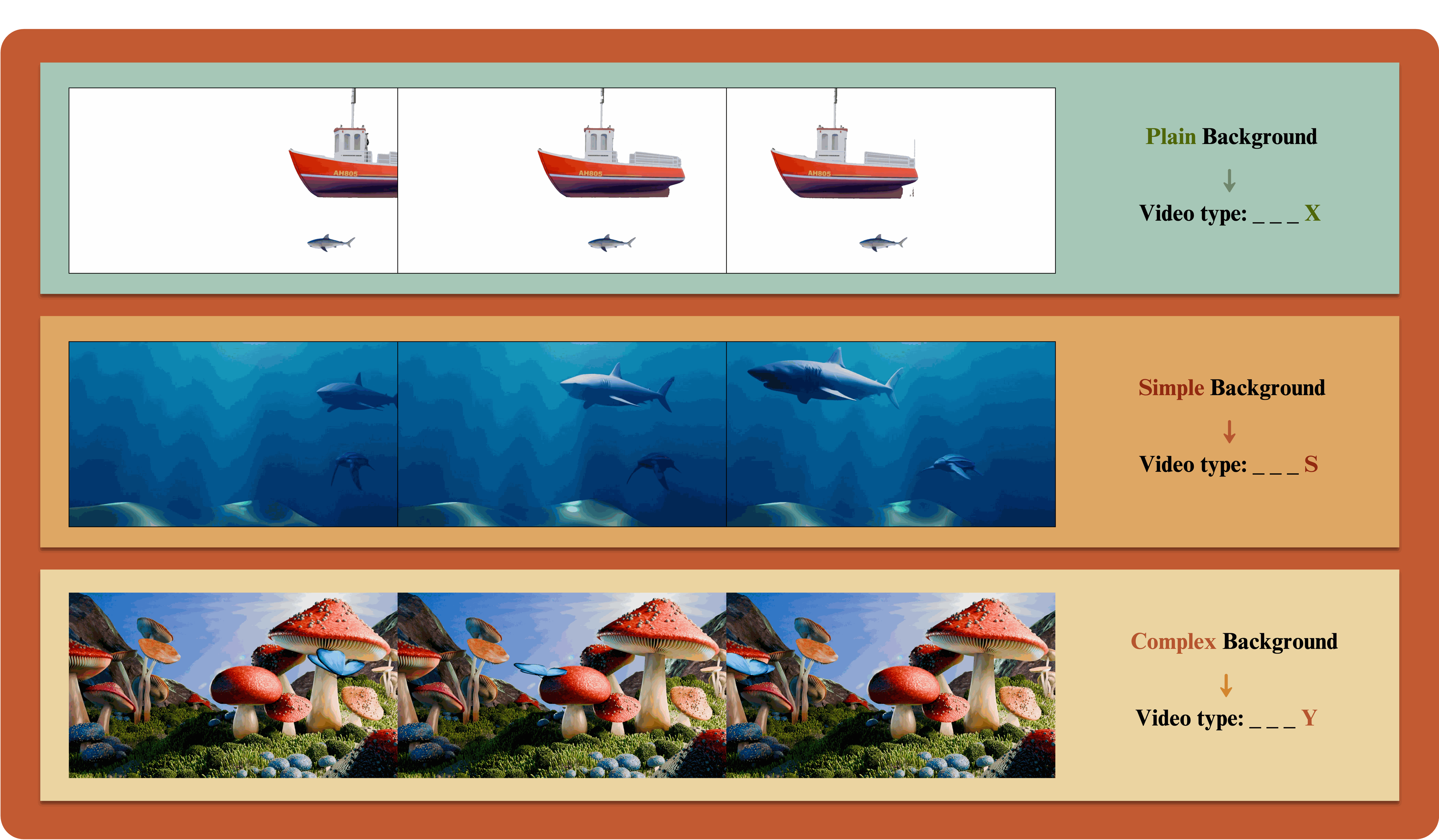
B.2.2 Quantitative breakdown of video types.
The inventory contains 328 planar and 241 three-dimensional videos. All 36 codes appear, with 4–51 clips per code; V2MC is largest. Table 4 gives the full source-by-code breakdown. The 85 segmented examples are processed variants of existing footage, so the total is not 569 independent source scenes.
| 2D/3D | Video Type | Blender | Internet | Captured | Segmented | Total | 2D/3D Total |
|---|---|---|---|---|---|---|---|
| 2D | A2SX | 0 | 0 | 0 | 11 | 11 | |
| A2SS | 10 | 6 | 0 | 0 | 16 | ||
| A2SC | 10 | 5 | 0 | 0 | 15 | ||
| A2MX | 6 | 0 | 1 | 8 | 15 | ||
| A2MS | 14 | 0 | 1 | 0 | 15 | ||
| A2MC | 17 | 2 | 1 | 0 | 20 | ||
| S2SX | 0 | 0 | 0 | 10 | 10 | ||
| S2SS | 10 | 5 | 0 | 0 | 15 | ||
| S2SC | 7 | 8 | 0 | 0 | 15 | ||
| S2MX | 8 | 0 | 0 | 8 | 16 | ||
| S2MS | 11 | 3 | 0 | 0 | 14 | ||
| S2MC | 16 | 20 | 0 | 0 | 36 | ||
| V2SX | 2 | 0 | 0 | 9 | 11 | ||
| V2SS | 10 | 7 | 0 | 0 | 17 | ||
| V2SC | 10 | 8 | 0 | 0 | 18 | ||
| V2MX | 13 | 0 | 0 | 7 | 20 | ||
| V2MS | 13 | 0 | 0 | 0 | 13 | ||
| V2MC | 43 | 8 | 0 | 0 | 51 | ||
| 328 | |||||||
| 3D | A3SX | 2 | 0 | 6 | 1 | 9 | |
| A3SS | 2 | 0 | 9 | 0 | 11 | ||
| A3SC | 3 | 0 | 7 | 0 | 10 | ||
| A3MX | 1 | 0 | 4 | 2 | 7 | ||
| A3MS | 3 | 0 | 4 | 0 | 7 | ||
| A3MC | 22 | 0 | 4 | 0 | 26 | ||
| S3SX | 1 | 0 | 8 | 2 | 11 | ||
| S3SS | 2 | 0 | 8 | 0 | 10 | ||
| S3SC | 2 | 0 | 8 | 0 | 10 | ||
| S3MX | 0 | 0 | 9 | 13 | 22 | ||
| S3MS | 1 | 0 | 10 | 0 | 11 | ||
| S3MC | 24 | 0 | 10 | 0 | 34 | ||
| V3SX | 3 | 0 | 2 | 0 | 5 | ||
| V3SS | 2 | 0 | 2 | 0 | 4 | ||
| V3SC | 3 | 0 | 2 | 0 | 5 | ||
| V3MX | 2 | 0 | 5 | 14 | 21 | ||
| V3MS | 3 | 0 | 5 | 0 | 8 | ||
| V3MC | 24 | 0 | 6 | 0 | 30 | ||
| 241 | |||||||
| Total | 300 | 72 | 112 | 85 | 569 | 569 |
Appendix C Details of Data Collection
Collection uses synthetic scenes, calibrated lab capture, uncalibrated real videos, and segmented derivatives. Manual selection and review remain substantial parts of the workflow.
C.1 Blender Simulation
Blender supplies diverse appearance and controllable trajectories. The appendix distinguishes artist-authored animation from force-based or analytically specified motion, an important distinction when interpreting “physical” ground truth.
C.1.1 Blender Toolkits and Asset Sources
BlenderKit mainly supplies environments and Sketchfab supplies animated foreground assets. Reusing rigs, animation cycles, materials, and scenes reduces authoring effort. The authors report selecting assets whose licenses permit the required reuse; the complete attribution table is retained. These licensing statements are the authors’ report, not an independent audit.
C.1.2 Two Motion Simulation Types
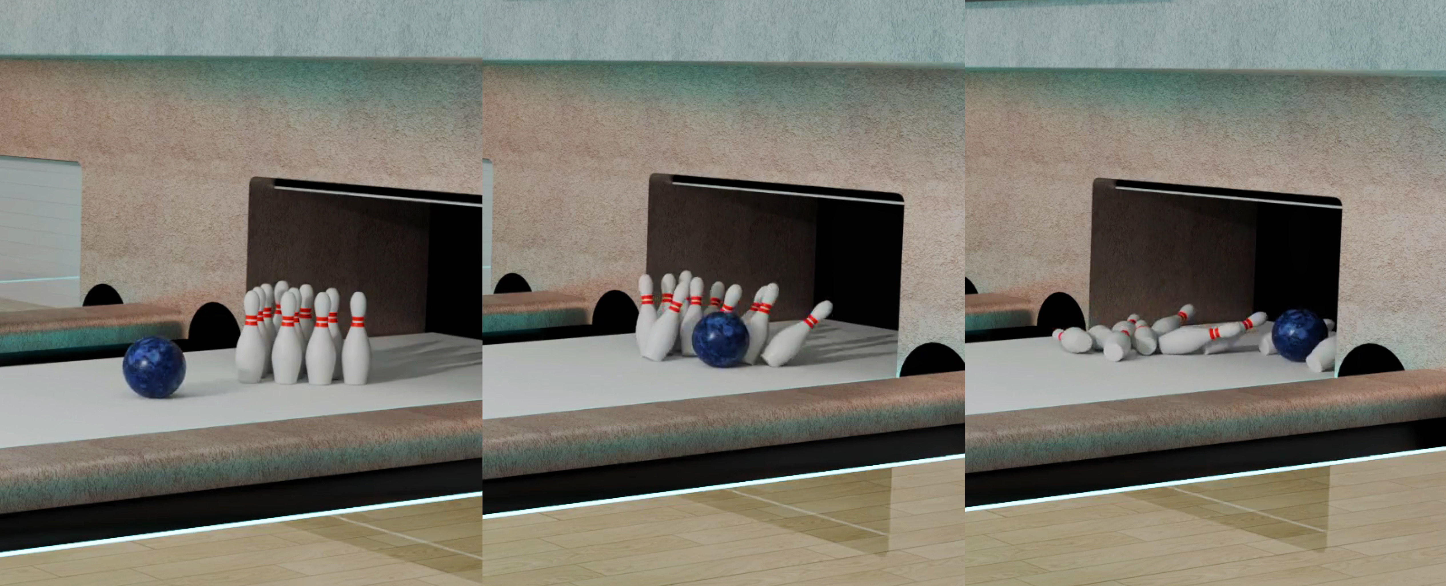
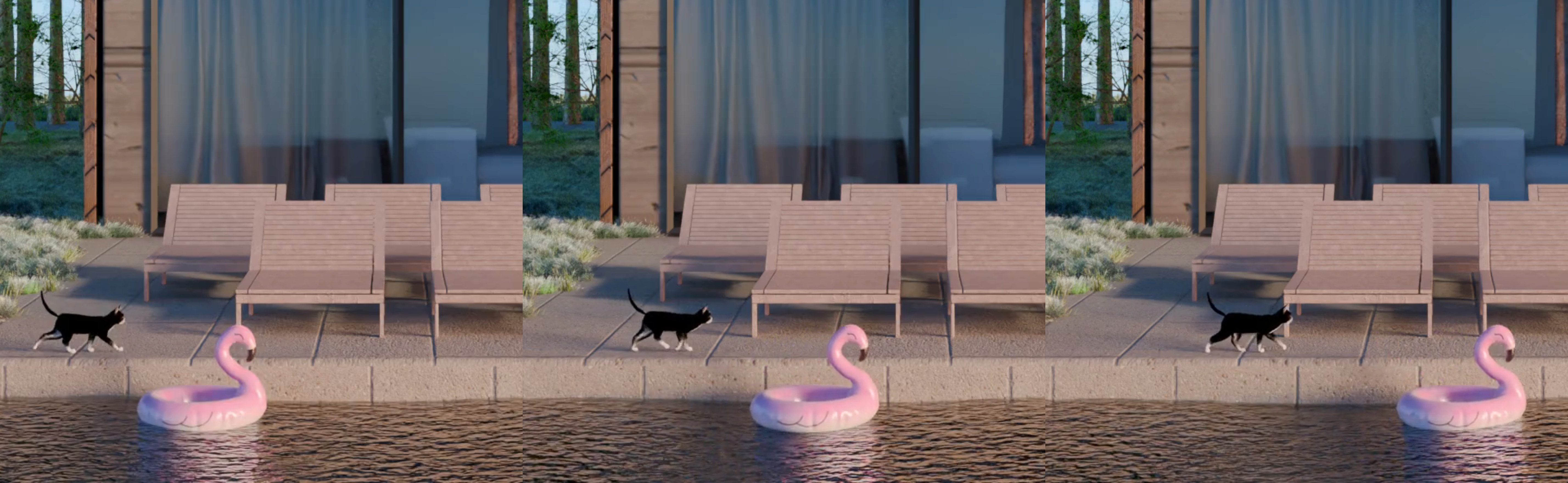
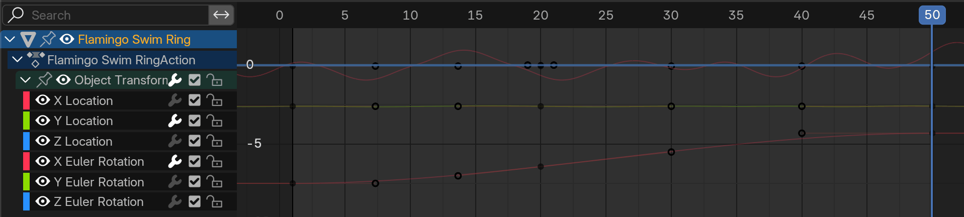
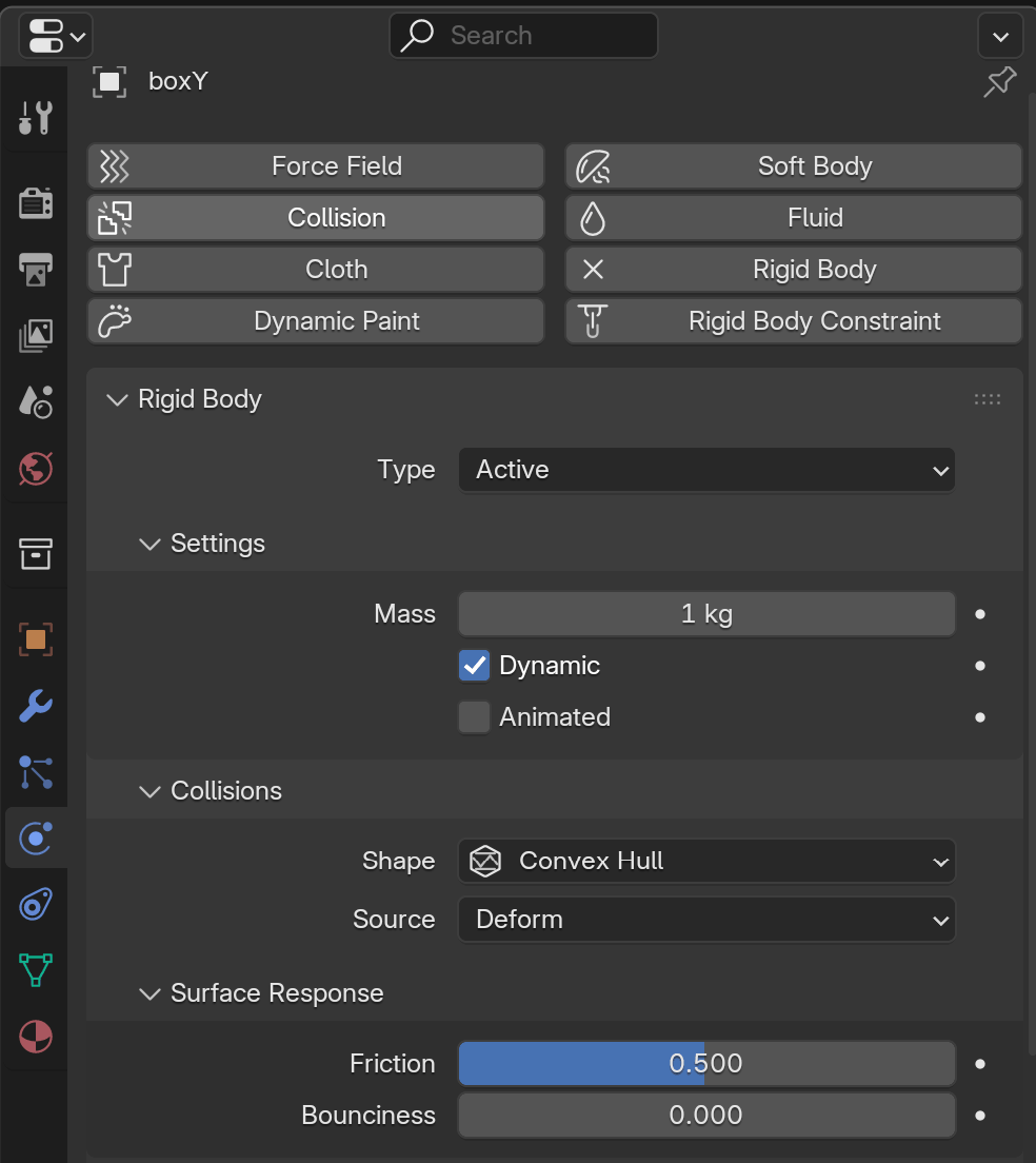
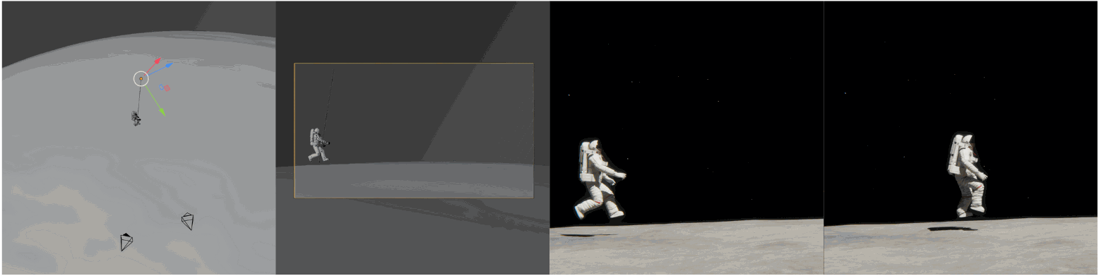
Keyframed motion can look plausible without following real physical laws—for example, lunar walking need not use lunar gravity. Force-based scenes use rigid-body simulation or explicitly prescribed kinematics. Consequently, the given prior and authored trajectory define the intended quantitative problem; familiar real-world constants are not always appropriate assumptions. The benchmark mixes these motion sources rather than representing every clip as calibrated Newtonian dynamics.
C.1.3 Blender Videos Construction
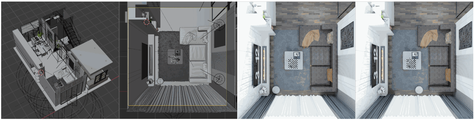
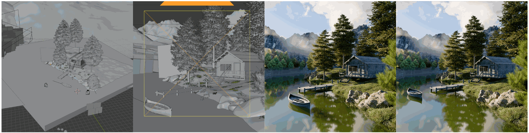
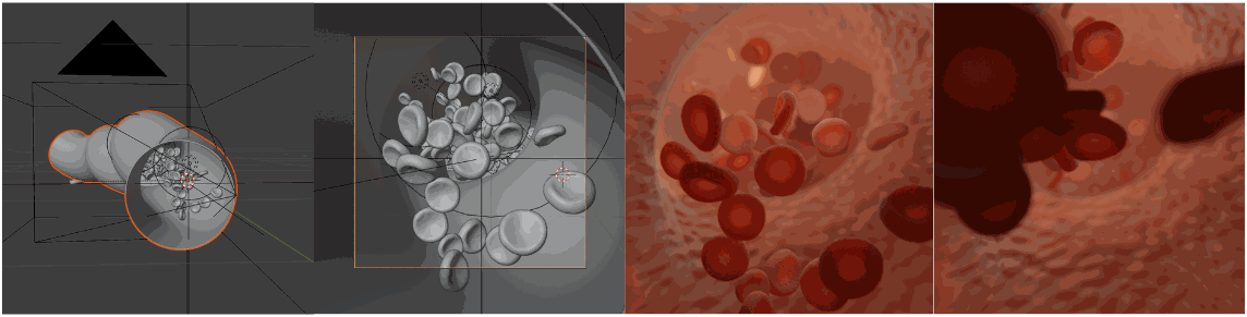
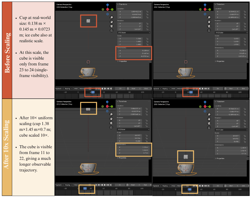
Approximately 125 base models and 81 base scenes are used; this subsection reports 312 Blender clips, whereas Table 4 reports 300. Background variants include both paired and independently constructed scenes. Some objects are uniformly enlarged to keep motion visible across more frames. Analytic scripts generate constant-speed or constant-acceleration trajectories; another pipeline samples an authored curve, computes cumulative arc length, and resamples it according to a chosen time–distance profile. Linear keyframe interpolation avoids default easing. Rendering varies resolution, frame rate, camera pose, materials, and lighting, with constant-rate H.264 exports. The six original script fragments and all accompanying formulas are preserved.
Equations
disp_y = 0.5 * ACCEL * (t ** 2)
new_y  = start_loc.y - disp_y
obj.location = Vector((start_loc.x, new_y, start_loc.z))
obj.keyframe_insert(data_path="location", index=-1, frame=f)
Equation
disp_y = VEL * t
new_y  = start_loc.y - disp_y
positions = []
for f in range(frame_start, frame_end + 1):
scene.frame_set(f)
pos = obj.matrix_world.translation.copy()
positions.append(pos)distances = [0.0]
for i in range(1, len(positions)):
d = (positions[i] - positions[i-1]).length
distances.append(distances[-1] + d)
total_length = distances[-1]
duration = (frame_end - frame_start) / fpsEquation
target_dist = speed * tEquations
ratio  = (target_dist - distances[i-1]) / (distances[i] - distances[i-1])
new_loc = positions[i-1].lerp(positions[i], ratio)
obj.location = new_loc
obj.keyframe_insert(data_path="location", frame=f)| Depth Technology | Time of Flight |
|---|---|
| Wavelength | 850 nm |
| Depth Range | *0.25–5.46 m (depending on depth mode) |
| Depth Resolution/FPS | Up to fps (WFOV), fps (NFOV) |
| Depth FOV | H V (WFOV), H V (NFOV) |
| RGB Resolution/FPS | Up to fps |
| RGB FOV | H V |
| Processing | NVIDIA Jetson Nano |
| IMU | Supported |
| Objects | Dimensions |
|---|---|
| 2 green tennis balls | d = 6.7 cm |
| 2 pink tennis balls | d = 6.7 cm |
| 2 white ping pong balls | d = 4 cm |
| 1 purple yoga ball | d = 52.2 cm |
| 1 soccer ball | d = 17.5 cm |
| 1 basketball | d = 23.2 cm |
| 1 red plastic ball | d = 7 cm |
| 1 orange plastic ball | d = 5.7 cm |
| 1 small whiteborad (slope) | 30.8 cm x 23.2 cm x 0.5 cm |
| 1 large whiteborad | 81 cm x 60 cm x 1 cm |
| 1 trashbin | 34.5 cm x 89.1 cm 59.9 cm |
| 1 tape | 10.1 cm x 10.1 cm x 4.8 cm |
| 1 white food box | 19.5 cm x 6.0 cm x 7.2 cm |
| stuffed toy 1 | 14.5 cm x 11 cm x 8 cm |
| stuffed toy 2 | 29.5 cm x 15.0 cm x 10.0 cm |
| stuffed toy 3 | 8.1 cm x 6.4 cm x 19.6 cm |
| 1 toy cookie | 8.0 cm x 8.0 cm x 1.8 cm |
| 1 cosmetic jar | 7.2 cm x 7.2 cm x 6.0 cm |
| 1 glass jar | 6.8 cm x 6.8 cm x 8.5 cm |
| 1 white cup | 8.6 cm x 8.6 cm x 14.5 cm |
| 1 pink water bottle | 6.7 cm x 6.7 cm x 19.5 cm |
| 1 marker | 13.5 cm x 0.8 cm x 0.8 cm |
| 1 black pen | 14.5 cm x 1. 2 cm x 1.2 cm |
| 1 green notebook | 18.6 cm x 8.8 cm x 1.5 cm |
| 1 white-covered book | 12.5 cm x 19.5 cm x 2.2 cm |
| 1 pencil case | 6.7 cm x 7.2 cm x 21 cm |
| 1 credit card | 85.6 mm x 53.98 mm |
| 1 deck of poker card | 9.8 cm x 6.3 cm x 1.8 cm |
C.2 Lab Capturing
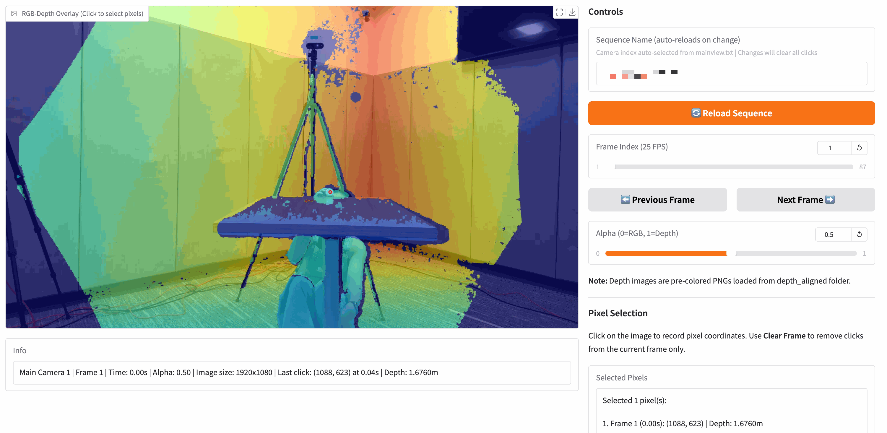
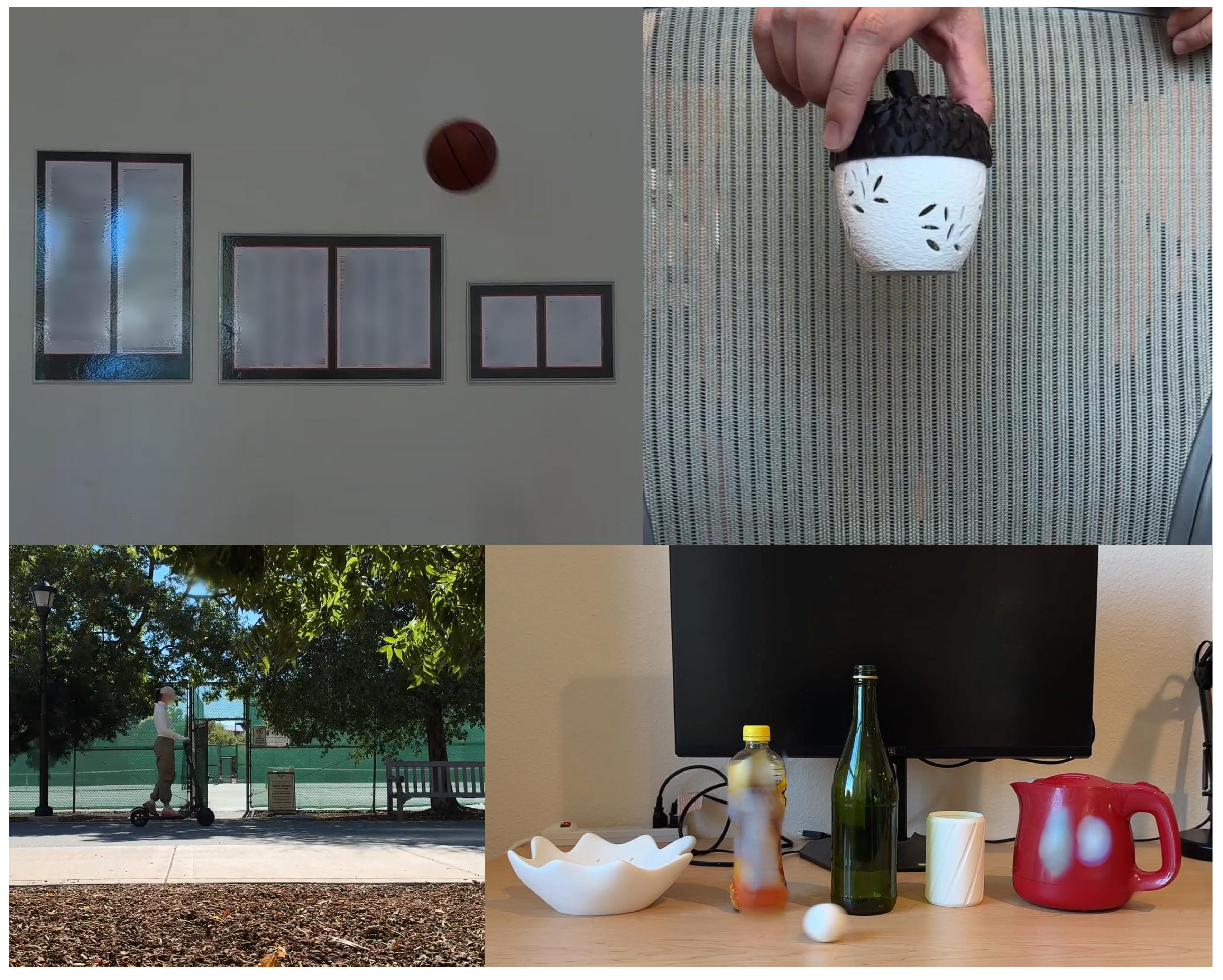
Four calibrated Orbbec Femto Mega cameras capture tabletop and larger motions. Checkerboard calibration initializes extrinsics, and synchronized RGB/depth streams are decoded and aligned. Automatic mask-averaged depth was unreliable under motion and incomplete sensor returns, so annotators use an interactive tool to select depth pixels. Physical object dimensions are measured before filming. These procedures improve control but retain manual localization and sensor-error sources.
C.3 Internet Scraping
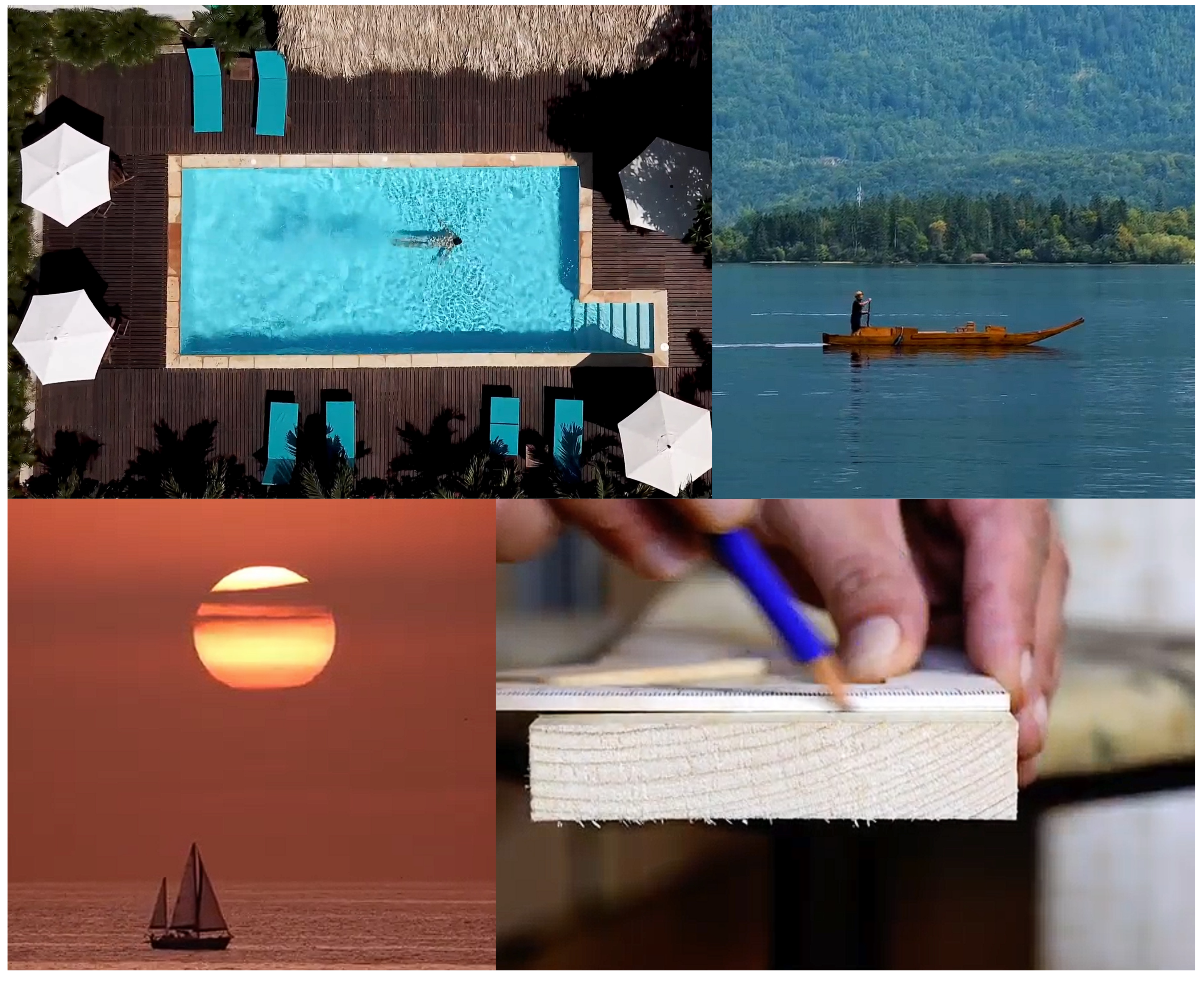
The Internet category combines 42 online clips with 30 author-recorded phone clips. All are restricted to planar tasks because calibrated metric depth is unavailable. Annotators use pixel measurements and approximate references such as gravity, lane width, or a credit card. The authors explicitly regard these labels as less precise than simulation or lab labels. Clips are manually selected, and identifiable faces or plates are blurred or masked.
C.4 Segmented Data
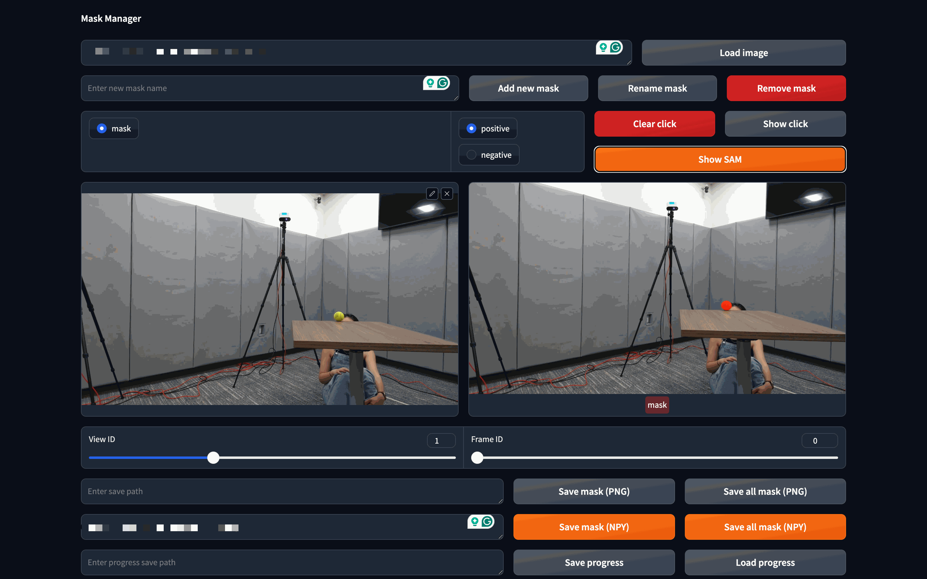
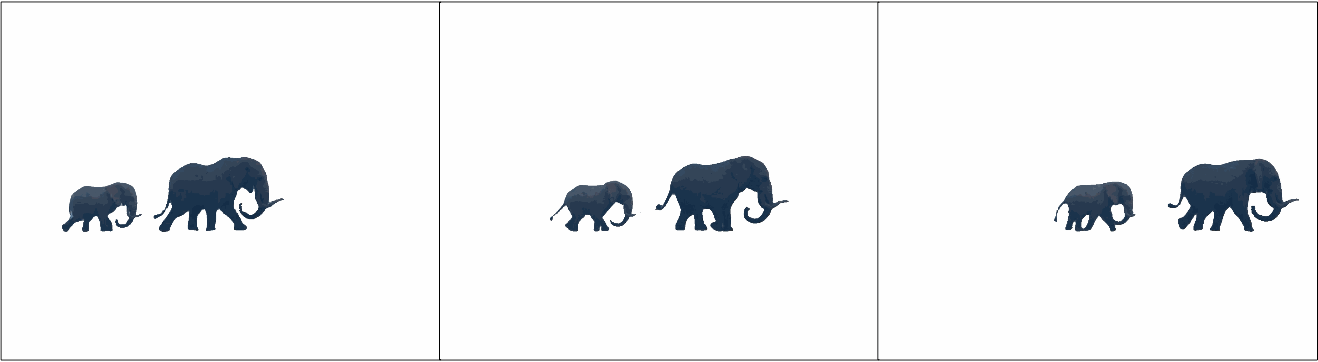
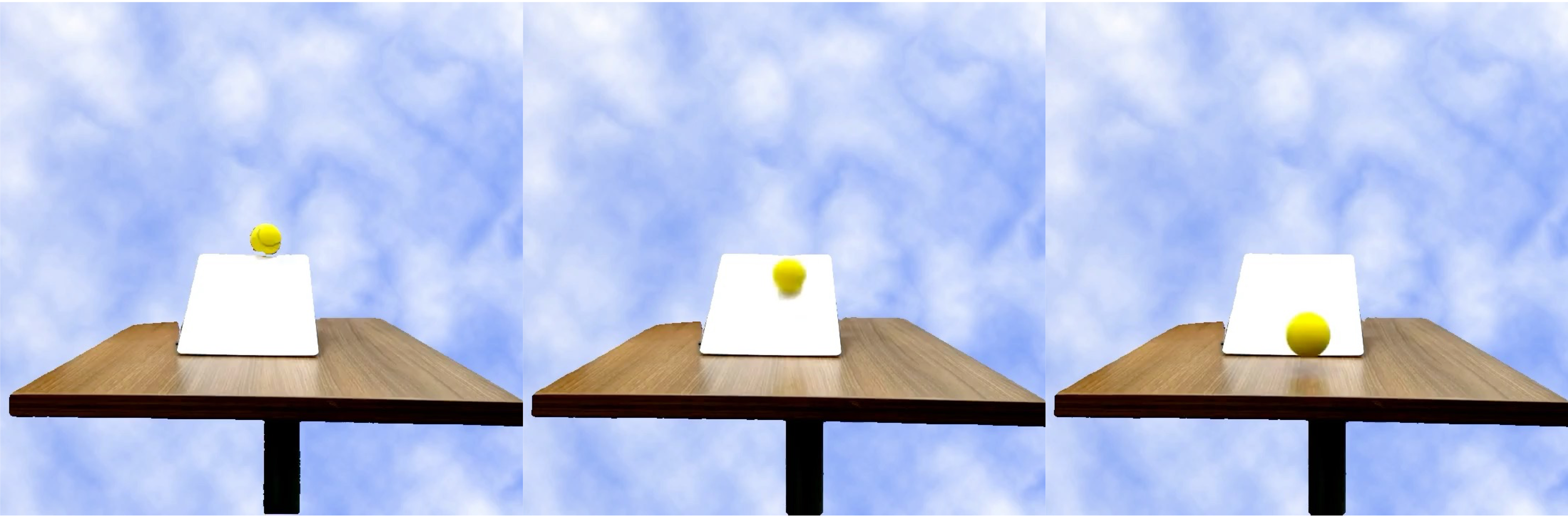
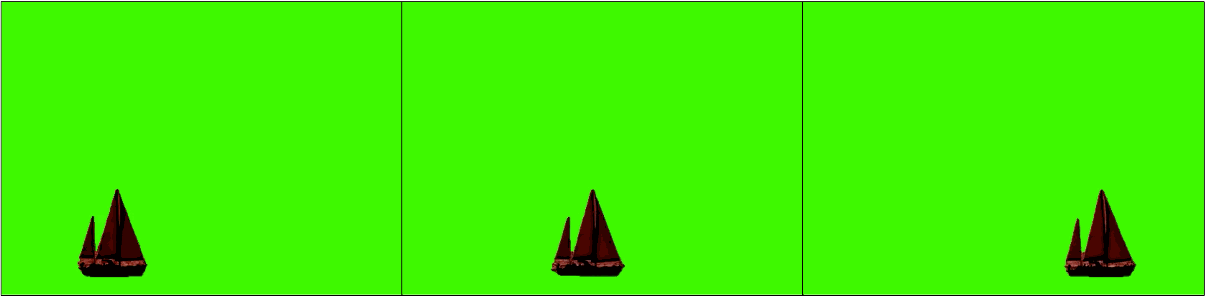
Grounding DINO supplies text-conditioned object boxes, and SAM 2 tracks and segments the target. Annotators add point prompts when automation fails. The retained interface and examples show background removal or replacement while preserving the target trajectory. Imperfect segmentation can still affect visual evidence even when the numeric annotation is reused.
C.5 Quality Control
Manual review removes severe blur, occlusion, difficult-to-model objects, and identifiable subjects. The authors report discarding roughly 3% of Blender candidates and 30% of lab candidates, while retaining 72 Internet-category clips. These are source-specific filtering rates rather than a measured residual annotation-error bound.
C.6 Ethical Considerations
The authors describe license checking, asset attribution, removal of personally identifying information, and content screening; relevant IRB documentation is said to be available on request. The edition preserves these disclosures without treating them as independently verified compliance findings.
Appendix D Details of Data Annotation
Annotation converts each source into numerical size, trajectory, velocity, acceleration, and geometric-reference labels. The full formulas and fourteen original code fragments remain available to inspect the implementation assumptions.
D.1 Blender Simulation
Blender labels are extracted from evaluated scene state. Size, displacement, speed, acceleration, camera distance, and inter-object distance use distinct definitions; the question must specify the intended quantity.
D.1.1 Size
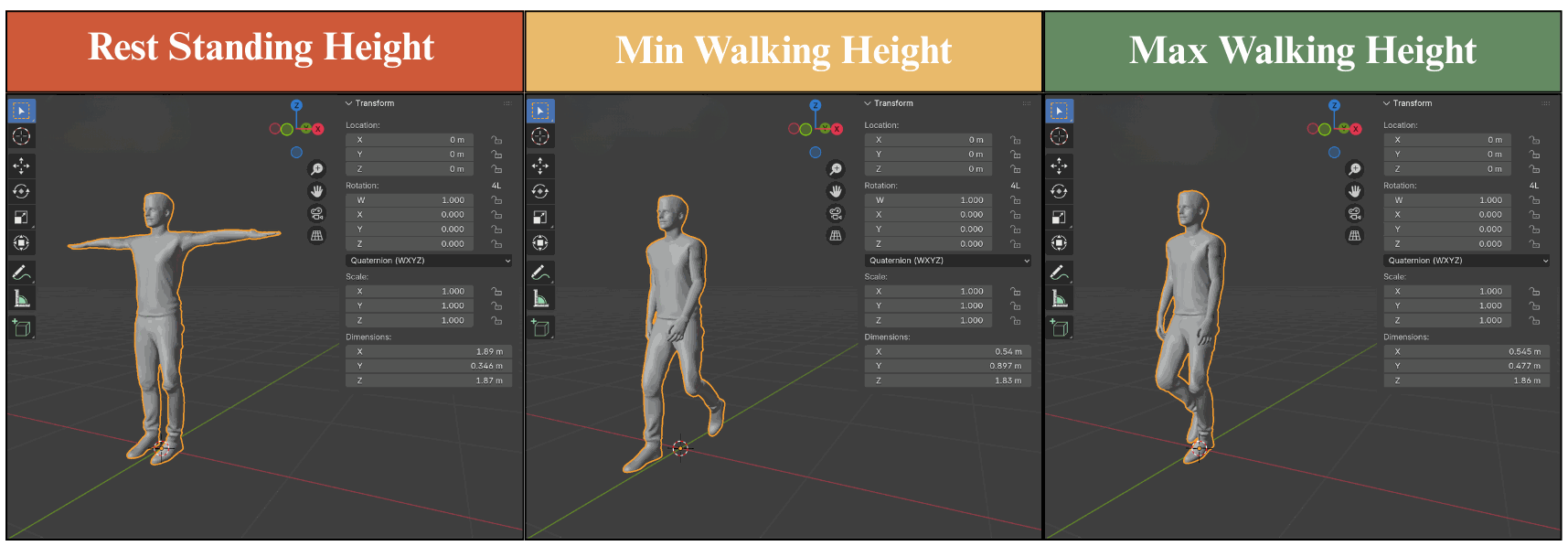
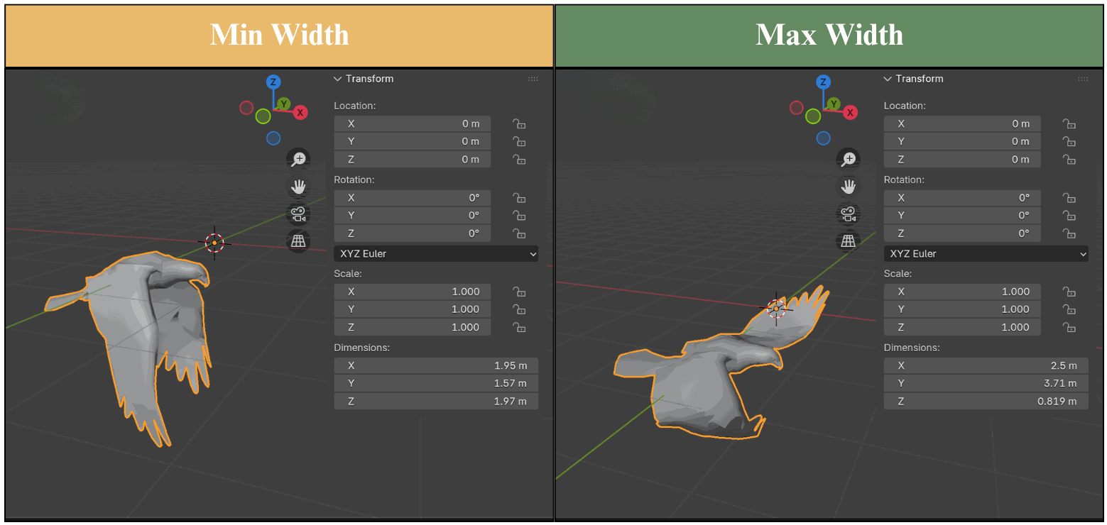
Most sizes come from world-space axis-aligned bounding boxes. Articulated humans receive rest, minimum walking, and maximum walking heights; flying animals receive minimum and maximum widths. The question and prior identify which configuration is intended. This accommodates pose-dependent extents instead of assuming every animated object has constant apparent size.
D.1.2 Displacement or Path.
Time zero is the render start frame, even when its Blender index is nonzero. Seconds are converted by rounding start_frame + fps × time. World-space endpoint positions yield displacement vectors, Euclidean 3D displacement, and specified planar projections. These endpoint distances should be distinguished from accumulated path length along a curved trajectory. Stored labels retain frames, times, endpoint coordinates, components, and scalar distances; the original code and equations show the exact conventions.
Equation
scene   = bpy.context.scene
fps     = scene.render.fps
f_start = scene.frame_start                      # may be 0, 20, 40, ...

def time_to_frame(t_sec: float) -> int:
    return round(f_start + t_sec * fps)
Equation
scene.frame_set(i)
loc = obj.matrix_world.translation.copy()          # (x, y, z) in world space
Equations
def displacement_world(obj, frame_start, frame_end, scene):
    # sample world-space positions at start and end
    loc_start = get_world_location_at_frame(obj, frame_start, scene)
    loc_end   = get_world_location_at_frame(obj, frame_end, scene)

    # displacement vector
    disp_vec = loc_end - loc_start
    dx, dy, dz = disp_vec.x, disp_vec.y, disp_vec.z

    # 3D displacement and horizontal (XY) displacement
    D_3D = disp_vec.length                 # sqrt(dx*dx + dy*dy + dz*dz)
    D_XY = (dx**2 + dy**2) ** 0.5          # sqrt(dx*dx + dy*dy)

    return {
        "frame_start": frame_start,
        "frame_end": frame_end,
        "loc_start":  loc_start,
        "loc_end":    loc_end,
        "dx": dx, "dy": dy, "dz": dz,
        "D_3D": D_3D,
        "D_XY": D_XY,
    }
D.1.3 Velocity and Acceleration.
Velocity is a finite difference of world positions; speed is its norm. The Blender acceleration diagnostic then differences scalar speeds, so it measures speed change rather than the full vector acceleration of a turning object. Mean speed and maximum relative deviation label approximately uniform motion; analogous signed-speed-change thresholds label acceleration or deceleration without changing frame-level measurements. The text excludes the initial undefined values, but the illustrative acceleration loop initializes speed to zero and must be checked carefully at the first transition. The scripts are preserved as supplied, not corrected or independently executed.
Equations
prev_loc   = None
prev_frame = None

for frame in range(frame_start, frame_end + 1):
    scene.frame_set(frame)
    loc = obj.matrix_world.translation.copy()   # p_i

    if prev_loc is None:
        vel_vec = Vector((0.0, 0.0, 0.0))
        speed   = 0.0
    else:
        dt      = (frame - prev_frame) / fps        # delta t_i
        disp    = loc - prev_loc                    # p_i - p_{i-1}
        vel_vec = disp / dt                         # v_i
        speed   = vel_vec.length                    # s_i

    write_per_frame_entry(frame, loc, vel_vec, speed)
    prev_loc   = loc
    prev_frame = frame
Equations
avg_speed   = sum(speeds) / len(speeds)
max_dev     = max(abs(s - avg_speed) for s in speeds)
max_rel_dev = max_dev / avg_speed if avg_speed != 0 else 0.0

if avg_speed == 0:
    # almost no motion
    ...
else:
    if max_rel_dev <= UNIFORM_SPEED_TOLERANCE:
        # approximately uniform speed
        ...
    else:
        # not uniform-speed
        ...
Equation
prev_speed = None
prev_frame = None

for frame in range(frame_start, frame_end + 1):
    scene.frame_set(frame)
    loc = obj.matrix_world.translation.copy()

    if prev_frame is None:
        dt    = 0.0
        speed = 0.0
        accel = None
    else:
        dt      = (frame - prev_frame) / fps
        disp    = loc - prev_loc
        vel_vec = disp / dt
        speed   = vel_vec.length

        if prev_speed is None:
            accel = None
        else:
            accel = (speed - prev_speed) / dt   # a_i

    write_per_frame_entry(frame, speed, accel)
    prev_loc   = loc
    prev_speed = speed
    prev_frame = frame
Equations
avg_accel   = sum(accels) / len(accels)
max_dev_a   = max(abs(a - avg_accel) for a in accels)
if abs(avg_accel) > MIN_ABS_ACCEL:
    max_rel_dev_a = max_dev_a / abs(avg_accel)
else:
    max_rel_dev_a = 0.0

if abs(avg_accel) <= MIN_ABS_ACCEL:
    # acceleration is very small -> closer to uniform speed / almost static
    ...
else:
    if max_rel_dev_a <= UNIFORM_ACCEL_TOLERANCE:
        if avg_accel > 0:
            # approximately uniformly accelerating
            ...
        elif avg_accel < 0:
            # approximately uniformly decelerating
            ...
        else:
            # numerically close to zero
            ...
    else:
        # not uniformly accelerated
        ...
D.1.4 Depth and Distance
Camera “depth” is defined here as Euclidean object-to-camera distance and serves as metadata or an optional prior, never an evaluation target. Object-to-object distances use object origins, a stable humanoid joint, or a parented helper object. Questions select full 3D distance or an explicit planar projection. The supplied world-position helper is illustrative: its pose-bone branch lacks an explicit armature-to-world transform, so the world-coordinate claim requires checking actual scene transforms and implementation. No simulator-label pipeline was independently rerun.
Equations
import bpy
from mathutils import Vector

scene = bpy.context.scene
fps   = scene.render.fps

def world_pos(obj_or_bone):
    """Return world-space translation of an object or a specific bone."""
    # For regular objects:
    if hasattr(obj_or_bone, "matrix_world"):
        return obj_or_bone.matrix_world.to_translation()
    # For pose bones (e.g., armature.pose.bones["Hips"]):
    return obj_or_bone.matrix.to_translation()

for f in range(f_min, f_max + 1):
    scene.frame_set(f)

    # Example: distance between entities A and B
    p_a = world_pos(entity_a)
    p_b = world_pos(entity_b)

    # Full 3D distance in world coordinates
    dist_3d = (p_a - p_b).length

    # Example planar distance in the XY plane (horizontal separation):
    # other planes (XZ, YZ) are obtained analogously in the full script.
    p_a_xy = Vector((p_a.x, p_a.y, 0.0))
    p_b_xy = Vector((p_b.x, p_b.y, 0.0))
    dist_xy = (p_a_xy - p_b_xy).length

    # Timestamp (seconds), assuming t = 0 at f_min
    t = (f - f_min) / fps

    # Log one line (frame, time, 3D distance, XY-plane distance, ...)
    write_to_text_block(f, t, dist_3d, dist_xy)
D.2 Lab Data Annotation
After unstable learned pose reconstruction, lab annotation uses calibrated back-projection of manually clicked centers and depth values. At least five adjacent frames support dynamic measurements; only frames needed for the chosen questions are annotated. Other cameras provide positions during main-view occlusion. The displayed finite differences describe vector motion, unlike the scalar speed-change diagnostic in the Blender subsection. Manual clicks, depth noise, and temporal sampling remain accuracy limits.
Equation
D.3 Internet Data Annotation
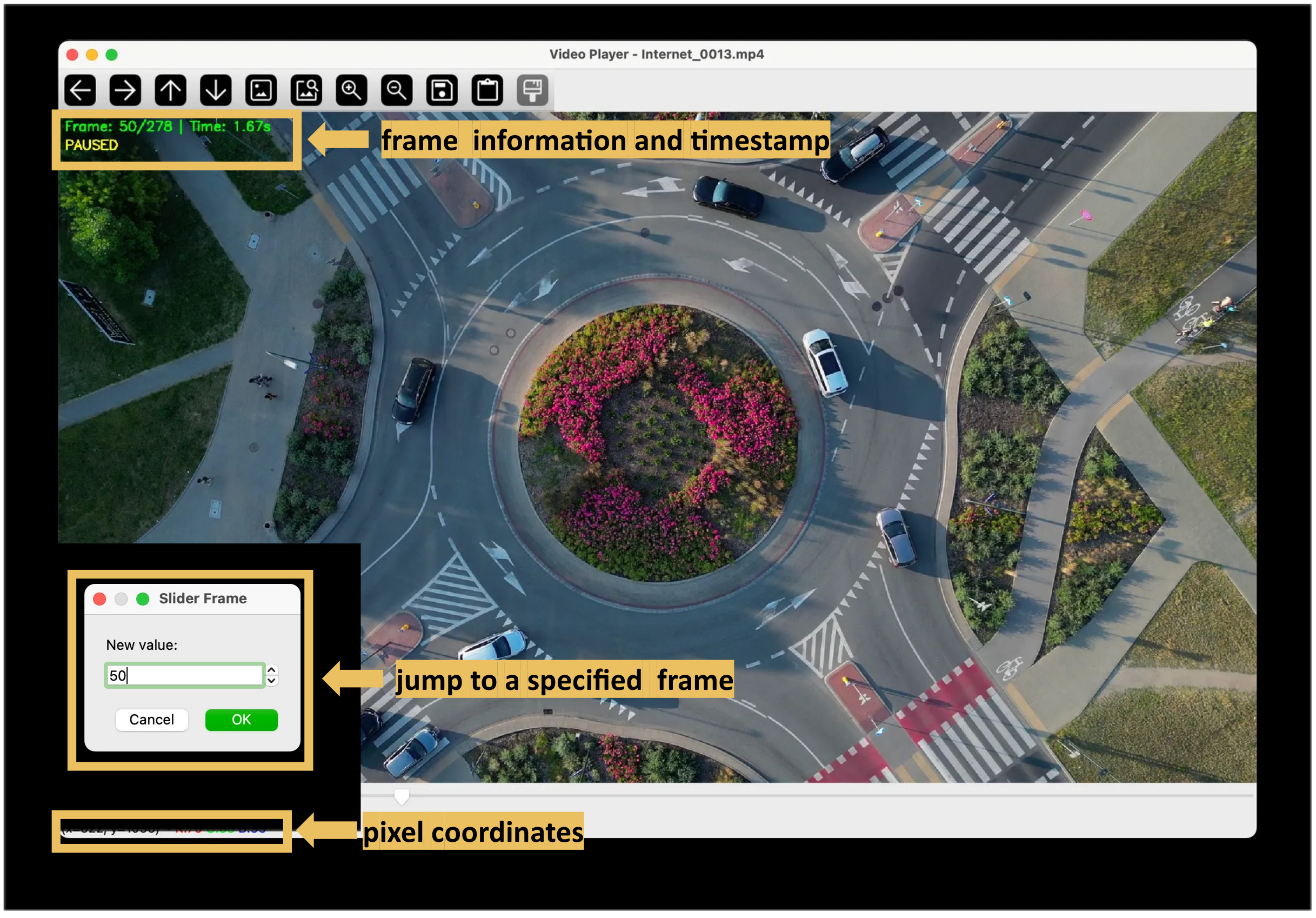
An OpenCV tool verifies frame rate, displays timestamps, supports frame stepping, and reports cursor coordinates. Annotators measure pixel sizes and trajectories, compute finite-difference velocities or accelerations, then estimate a positive world-length-per-pixel factor from the available prior. Multiplying target pixel quantities by this factor produces labels. This construction relies on the planar/common-scale assumption and on the accuracy of the chosen real-world reference.
Equations
D.4 Segmented Data
Segmented variants reuse the original labels because background editing is intended to leave target geometry and motion unchanged. This avoids a second numeric annotation pass, while introducing dependence between variants from the same source clip.
Appendix E Vision-Language Models
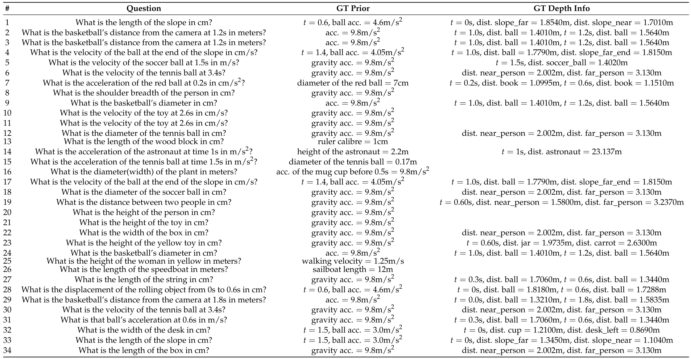
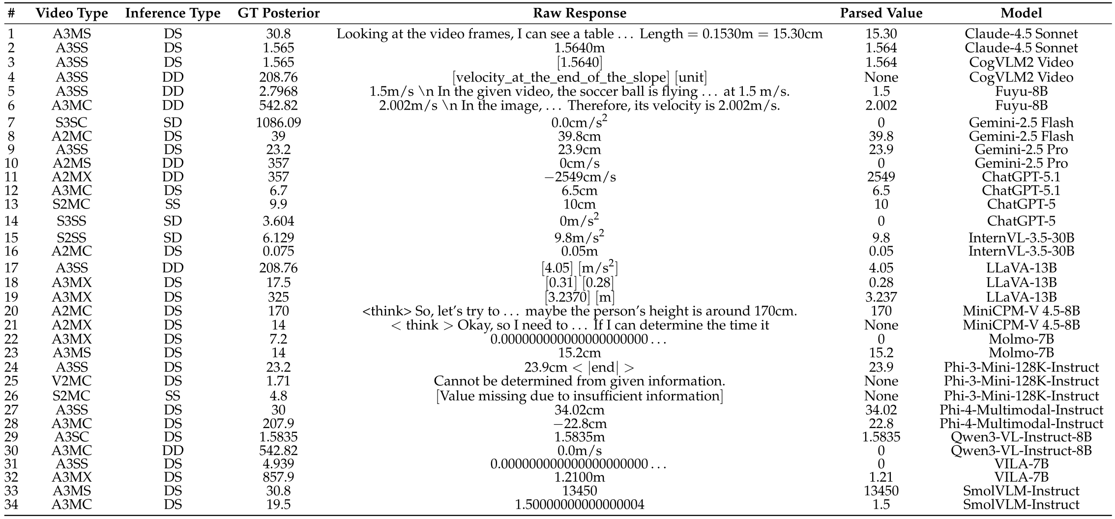
The appendix records provider names, API model identifiers, and open-model families. Some systems ingest frame sequences, while MiniCPM-V and CogVLM2 accept native video inputs. Model naming and cited versions are not uniformly aligned—for example, Qwen3 entries cite a Qwen2.5 technical report—so replication should use explicit deployment identifiers rather than infer checkpoints from bibliography titles. The original two large input/output example tables are retained, rotated for readable viewing.
Appendix F Prompt Design
The shared input combines video frames, a video-analyst system instruction, physical prior and optional depth, the question, and a numeric-output reminder. Videos are normalized to 480p while retaining frames; the claimed small spatial-resolution effect comes from preliminary exploration, not a full reported controlled study. A pilot compares five prompts on fifteen videos. Temperature is zero where supported, with hosted defaults otherwise. The instruction suppresses explanations in the final output, but does not establish identical internal reasoning budgets across models.
Appendix G Answer Retrieval and Parsing
The parser accepts concise numeric answers, otherwise seeks a final-answer delimiter, strips common unit text, and takes the last numerical match after applying an absolute value. Qualitative answers and unsuccessful retries become failures. This heuristic can select an unintended number or obscure a sign/unit error; formatting adherence is not equivalent to physical correctness. The example tables expose raw responses alongside parsed values. Main-text and appendix statements differ on whether failed questions are excluded or assigned zero when aggregating scores.
Appendix H Human Study Details.
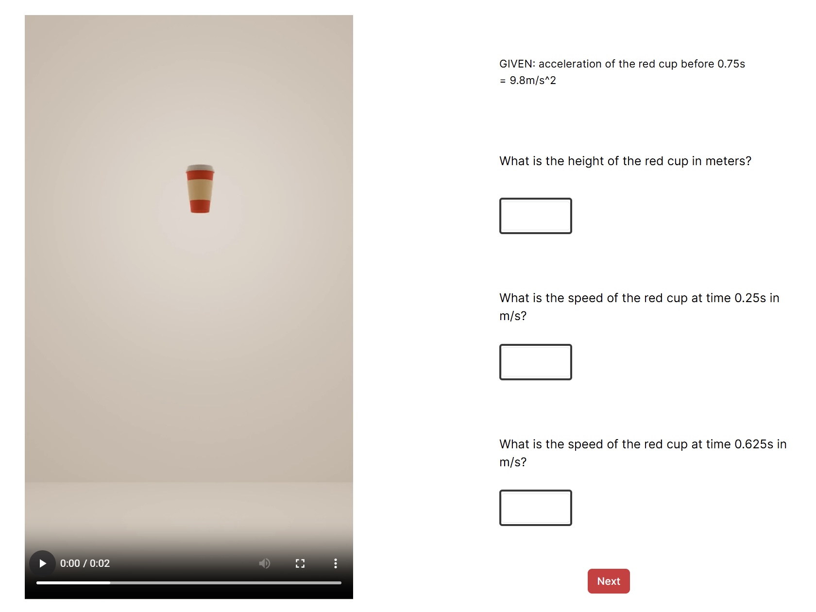
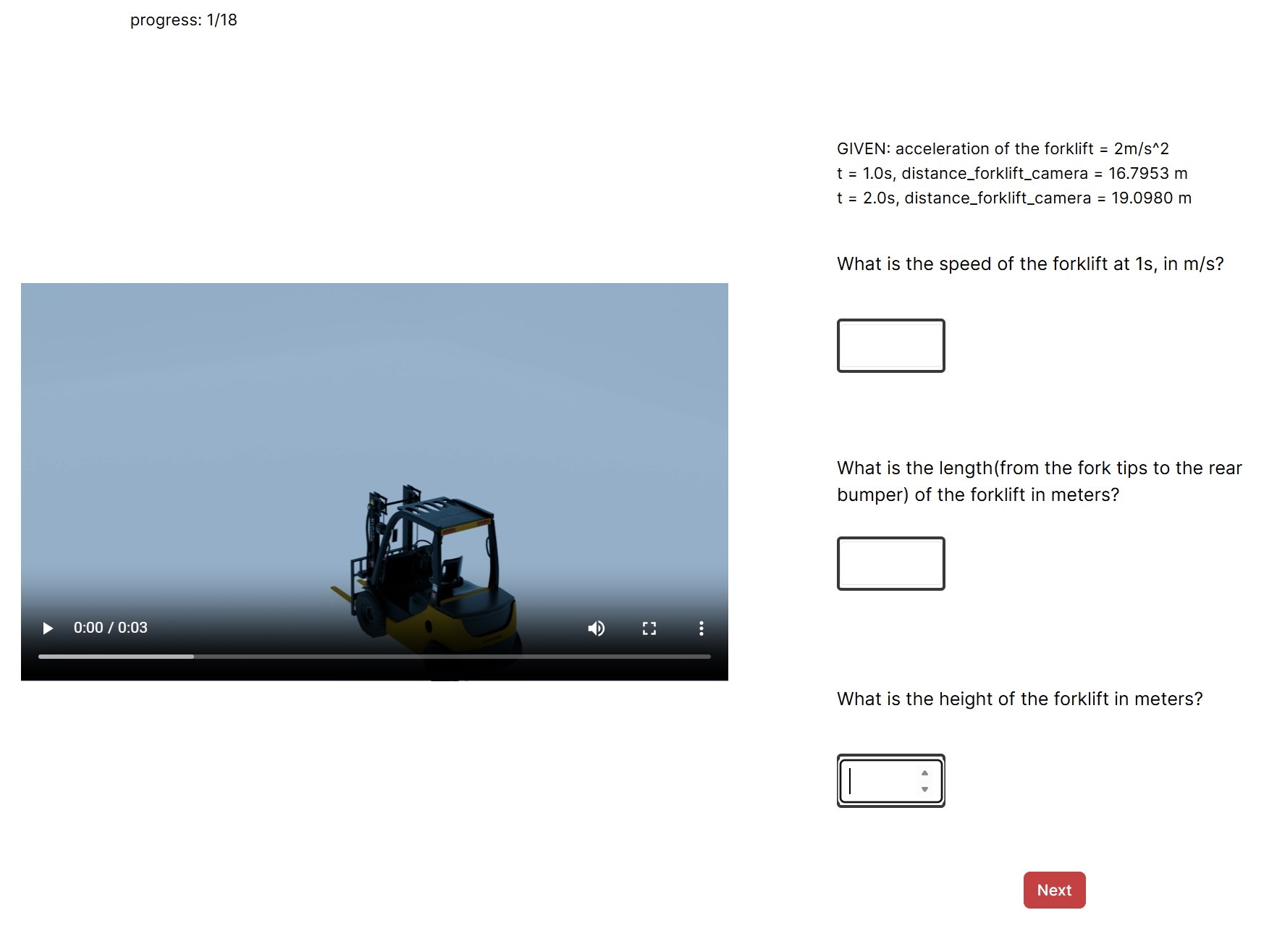
The human study uses Gorilla survey interfaces with the same question wording and priors. It offers a reference sample of human estimation, rather than a population ceiling or a fully matched model experiment.
H.1 Participants
Participants include undergraduate, graduate, and PhD researchers, with some technical training and some overlap between 2D and 3D surveys. They choose their own strategy, from intuition to explicit calculation. The appendix does not report a numeric participant count, limiting assessment of sample precision and representativeness.
H.2 Task Construction and Experimental Design
Each participant sees eighteen videos, one sampled from each category of the assigned dimensionality, with one to three questions per video. Playback, pause, and replay are allowed; scrubbing is restricted to whole seconds. This is a different observation interface from models receiving frame sequences, and different participants see sampled clips. Assertions of comparable evidence should be interpreted with those interface and sampling differences.
H.3 Evaluation Metric
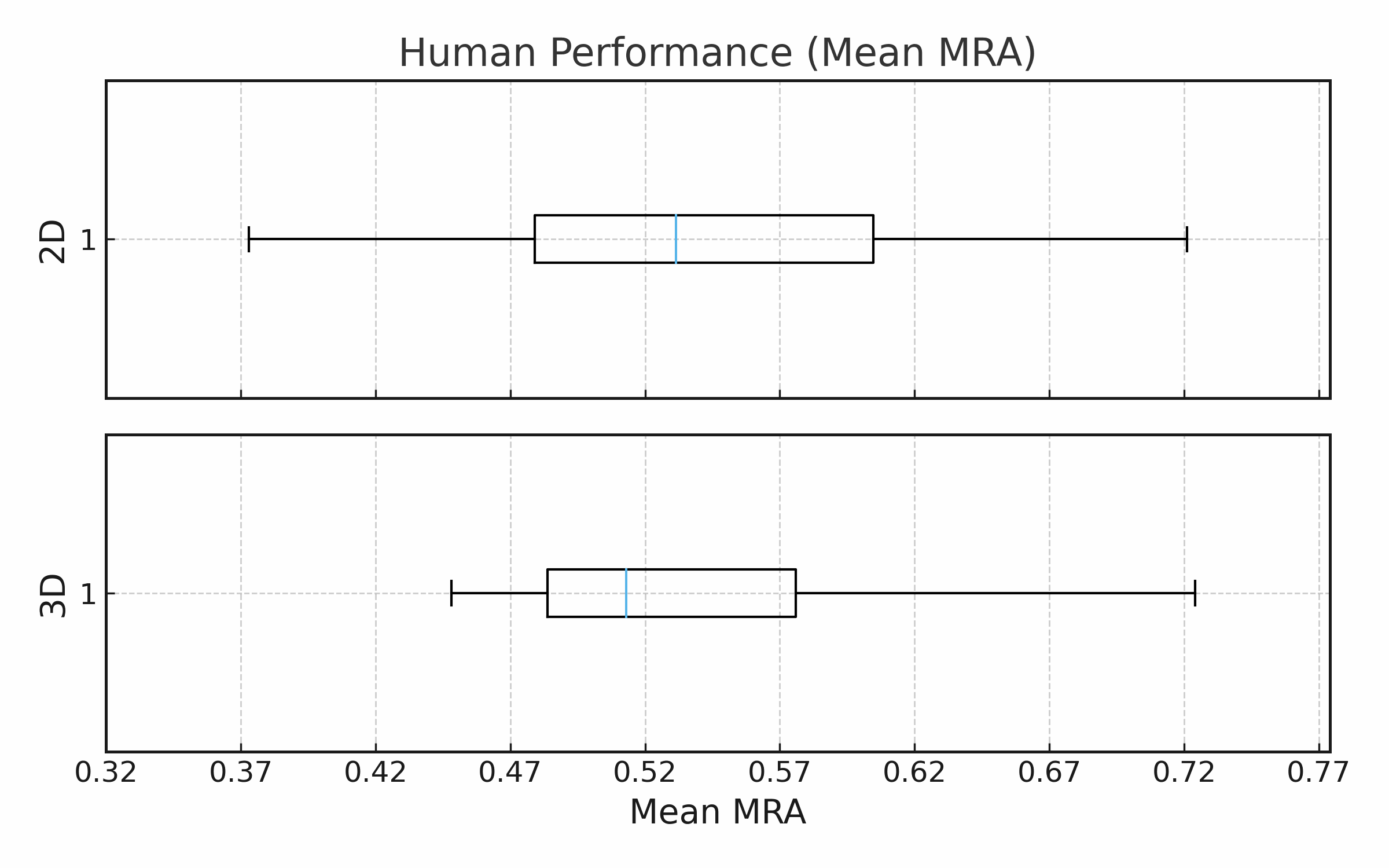
Question MRA is averaged within each participant, and Figure 39 shows the distribution of participant means. This aggregation differs from the four-category average reported for models. The source says the same metric is used, but the inconsistent threshold sets elsewhere prevent determining a single unambiguous implementation from the paper alone.
H.4 Results and Observations
The best observed participant scores are 0.721 for 2D and 0.724 for 3D. The text reports cross-dimensional consistency among repeat participants without a numerical correlation estimate. These maxima describe this small sampled study, not a universal upper bound. The appendix’s statement about average humans not outperforming models also needs context beside Table 1’s human 55.6 versus best-model 53.1 on different evaluation populations.
Appendix I Sketchfab Model Sources
The complete two-page Sketchfab attribution table preserves model names, creators, and asset identifiers. It documents the reused foreground assets and supports tracing the synthetic scenes to their reported sources.
| Model Name | Author | Model ID |
|---|---|---|
| Supermarket trolley broken | kreems | 7f460877380349f8886280a596253034 |
| supermarket 1 | amogusstrikesback2 | ca1def2b7be544068def3cec5852c67e |
| Pool Table (Animation) | Yanez Designs | 0f2ae181a2dd4b00a6ec25073692037f |
| Bowling Pack (Bowling Pins & Ball) | EverZax | 52743c4714c14211ac71d2fe1e5c8da3 |
| Bowling Club | tiunov.se | 0b8fae45fcda4fe78f93bb2a899401a6 |
| Elephant | planeta-elefante | f8778fc3d161481abba7ec23a8ddd1e8 |
| Walking Astronaut | Unknown Animaker | d9062a2003df422abdafdc02afdac085 |
| Mr Man Walking | Instinto Ideal Studio | 98ccac2b0e2845789b6f789978ca06ed |
| Jupiter & satellites | Sakado | 379fd77b970c4821898c05c483913dec |
| Model 92A - Great White Shark | DigitalLife3D | 702e7b53637f4ded9ca479a8124e810d |
| Model 95A - Adult Leatherback Sea Turtle, ”Mac” | DigitalLife3D | 4974c93644a24da280fde68cba74a12d |
| Model 69A - Striped Bass | DigitalLife3D | 35be3af9a7c4441c98109e5562d36c09 |
| Underground Parking Lot | Janis Zeps | 0ad5c221525b4bbba3a164c6235d28b8 |
| Airport Car | Jungle Jim | 29d1c6260b134a3baf5231f34de1b24f |
| Airport Catering Truck | rwy00 | 289f4e2cfa3f4722b0476b1fc37681d8 |
| Towel | TheSpacePunk | 6edc341457e44603ab351470ab800493 |
| Plain Mug | LightSwitch | 19c8fe5702b544d0a1409d3dac1cf90e |
| Flour ARIDLL | fwild | d40db94d92ab4e7a82a1c199312f3985 |
| Milk | Multipainkiller Studio | 5e8d71045e2040ba8f6619d86d204cf5 |
| Apple [Scan] | hoxsvl.scan | facb1aa6928c4f8f82d87a019b9f134e |
| PACKAGING EMPAQUE DE HUEVOS | willinando1w08 | cd51c5d25bbd4370881aebd3648cfe8c |
| Kitchen Pack | GRIP420 | a513f2e85bc94ae5b6d8cbd74909e3c4 |
| Kitchen Tools | anybody | 417e3873fcb34f7ab9744506d7bcc838 |
| Coffee Shop Cup | David Zerba | 37e6805f2b7a4158a1d61fe75f8e2a33 |
| Cup | Dmytro Nikonov | 7d450bb714034fceaa7b59a0e564f46b |
| Bird Animations Alex | ahitch3 | 081fa7f0cfd649b9b07babb4c619acc7 |
| Dove Bird Rigged | FourthGreen | 6b91be2a28fb4404a2d57d5ca98bd4dc |
| POLICE CAR - Belgian VW Transporter | Mickael Boitte | 35eaf9505e13464385404402ad865508 |
| Jo on Bike - Rigged & Animated | NEEEU Spaces GmbH | 36ee5344e81149858a664cde9f98e835 |
| Simple Factory Scene | Pickeri | 804fbe0cd1fa44fa9ca86ae42c82d63d |
| Car | Paulius | a619dd25a6c04af0b2d8730aa1cb058b |
| Basketball Court | tiunov.se | 5faad7b528124907ab82732ed0c6b743 |
| Basketball NBA Championship Official Trophy | johnnokomis | 04f6f1135ffb48749c43c9c20c75fc19 |
| Bouncing Basketball | Maurice Svay | b8731a2fda6849c9a164d1966dc16ff8 |
| Zen Japanese Tea House with Go Board | winters810 | a1e95e5efee349a693f30eda32401aef |
| Chinese Chess | chung_the_artist | 7ad0f4f0ebbc455d9e9f829c956dda80 |
| paper airplane | vesicalsnail | 0967ab4a9c654a569a13ea1f8d9dca0c |
| 3d soccer ball | BlenderMaster | 0400146e0e3c4d8f8b57bfa06d7dfb4c |
| Cardboard Box | Pricey1600 | 4e622ef1a09c43e28a49d9fa37f9eeee |
| Tennis Ball Low-poly PBR | MaX3Dd | e5c2b0e5860549acaa2dfe8b764d5f94 |
| Old Camera Bag .::RAWscan::. | Andrea Spognetta (Spogna) | 788f8b75874f417ebde498ffd231410c |
| Animated ROBOT SDC | SDC PERFORMANCE | 3d127f327a6c4033a32b810b5fb071ed |
| Gift Box | local.yany | 83296611584143a3afad6c0d0c0a4227 |
| Sci-fi Box | Igor_K. | ca415724f32043489fcab2ec74582619 |
| Cat Walk | LostBoyz2078 | 915680200c064815bba75e008ba9efb5 |
| Deer walk | LostBoyz2078 | 229ba6ba0d1e4811ab89382f74601e16 |
| Horse | kenchoo | 86d47bdcd5ab41238ba44547e4d21f9c |
| Horse Walk | Amitesh Nandan | 93b53ddcec414592842753d1819f3133 |
| Rabbit Rigged | FourthGreen | e7213589744d436b9d96e2dbb31198a5 |
| phoenix bird | NORBERTO-3D | 844ba0cf144a413ea92c779f18912042 |
| First Aid DX2 - 300 Followers Celebration | re1monsen | c5ddfa9e6309403083bbce60bdcc3d71 |
| Nathan Animated 003 - Walking 3D Man | Renderpeople | 143a2b1ea5eb4385ae90a73657aca3bc |
| Chernovan Nemesis | Swiss_Fox | c6c91c73e93444f4b72d6c24db778e73 |
| Dragon Fly | LostBoyz2078 | 1443a7efe5d5450b8db4c15d8ff5c343 |
| Borboleta Azul - Butterfly | Lancaster Modelagem 3D | ab9192b6bc8f49e3baed63e984c7073a |
| Blue Whale - Textured | Bohdan Lvov | d24d19021c724c3a9134eebcb76b0e0f |
| jellyfish | yanix | d06a5a553fe641ab92f720527b2278f3 |
| Koi Fish | 7PLUS | 236859b809984f52b70c94fd040b9c59 |
| Running Raccoon Animation | Santrez | bfce4d4815234c39bcf012352e52c27e |
| (FREE) Cyberpunk Hovercar | Lionsharp Studios | 3205b1075bb44ffc826bce0c2a04d74c |
| White Eagle Animation Fast Fly | GremorySaiyan | 30203bf39e5145f19c79e83c550139d3 |