At a glance
The paper separates learning audio features from reconstructing sound. First, a masked-prediction encoder learns with density-adaptive gates. Second, scalar quantization and an audio decoder convert those features into compact tokens and reconstructed waveforms. The proposed packing gives 47.5 tokens per second. Reversibility applies to packing the quantized indices, not lossless recovery of the original waveform. The paper describes preliminary qualitative evaluation rather than a comprehensive quantitative codec comparison.
1 Hybrid Discrete-Continuous Speech Representations via JEPA with Density Adaptive Attention
The two stages serve different goals: learn reusable acoustic representations first, then learn a practical discrete audio interface and reconstruction decoder.
1.1 Overview
A JEPA encoder predicts masked latent features, while a Gaussian-mixture-based gate adjusts which temporal features receive emphasis. After pretraining, a quantizer and decoder are trained for audio reconstruction. Keeping those stages distinct makes it possible to study representation learning without immediately demanding waveform fidelity.
1.2 Motivation: Why JEPA for Speech?
A codec must retain details needed to reproduce sound, whereas a representation for understanding may ignore some of them. The staged design tries to reduce that conflict. Proposed uses in speech recognition, synthesis and voice conversion are possibilities; the source does not report complete downstream evaluations of every suggested application.
2 Stage 1: Self-Supervised JEPA Encoder with DAAM
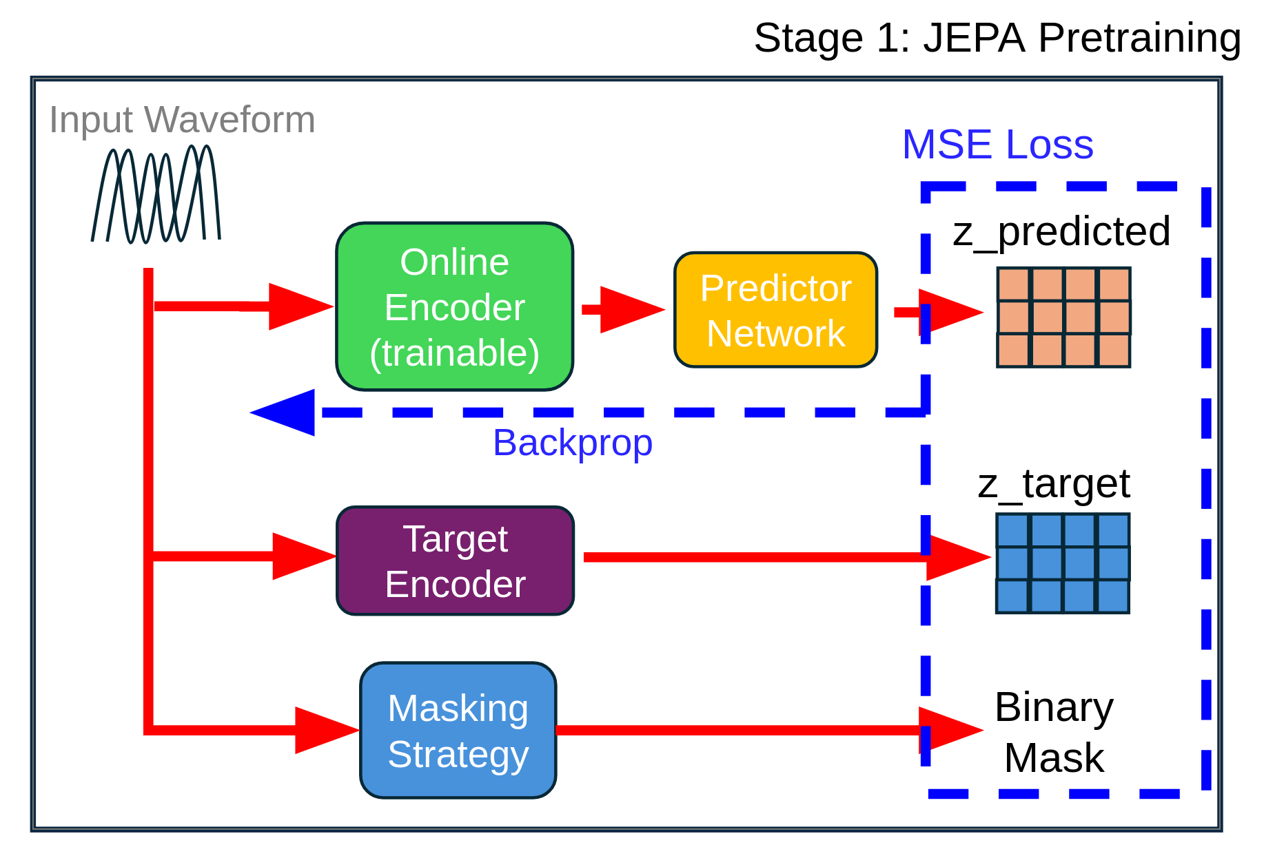
Stage 1 performs feature prediction rather than waveform reconstruction. Mask placement, the target-encoder update and the density gate are the main implementation choices.
2.1 JEPA Masking Strategy
Contiguous temporal blocks are hidden from the predictor, encouraging prediction across longer gaps than independent-frame masking. The mask fraction and span lengths determine the difficulty. The source applies feature masking after the audio encoder; this is not equivalent to withholding all masked waveform content from every earlier encoder operation.
2.2 Density Adaptive Attention for Temporal Feature Modulation
DAAM forms a temporal gate from learned Gaussian-mixture densities. It asks which feature values are statistically salient under that parameterization, rather than comparing every time position with every other position. The complete formula and architecture remain below.
2.2.1 Mathematical Formulation
The gate computes temporal statistics, positive mixture scales, standardized deviations and log-density scores, then combines them stably before modulating features. Its one-channel projection supplies a shared temporal gate to the full feature tensor. Numerical safeguards and floating-point precision are part of the implementation; the mechanism does not prove that high-density or unusual values are always linguistically meaningful.
Equations 1–8
| (1) | ||||
| (2) |
| (3) |
| (4) |
| (5) |
| (6) |
| (7) |
| (8) |
2.3 JEPA Encoder Architecture
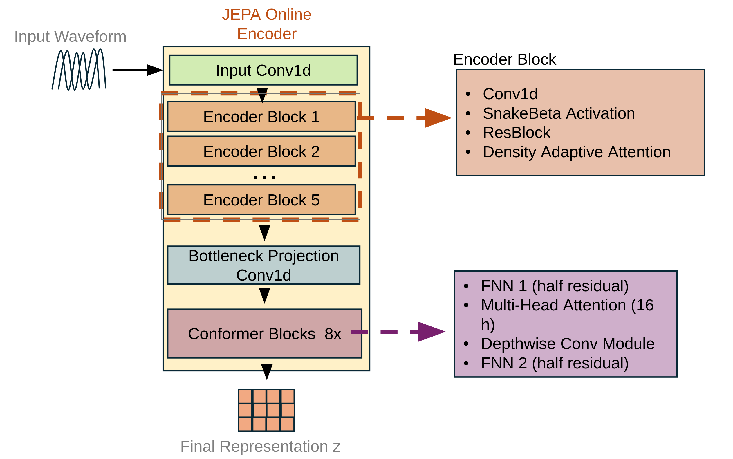
The online encoder is updated by gradients. An averaged target encoder provides the features the predictor should match. Both process the audio before the specified feature-mask/predictor step. The target branch is a training device and is unnecessary for ordinary inference.
2.3.1 Convolutional–Transformer Hybrid Design
Strided convolutions compress time, and Conformer blocks combine attention with local convolutional processing. The resulting frame rate is about 2.5 Hz. The source text is inconsistent about whether DAAM follows Conformer blocks or only encoder convolutional blocks; keep that wording separate from what the architecture figure and implementation show.
Equations 9
| (9) |
2.4 JEPA Predictor Network
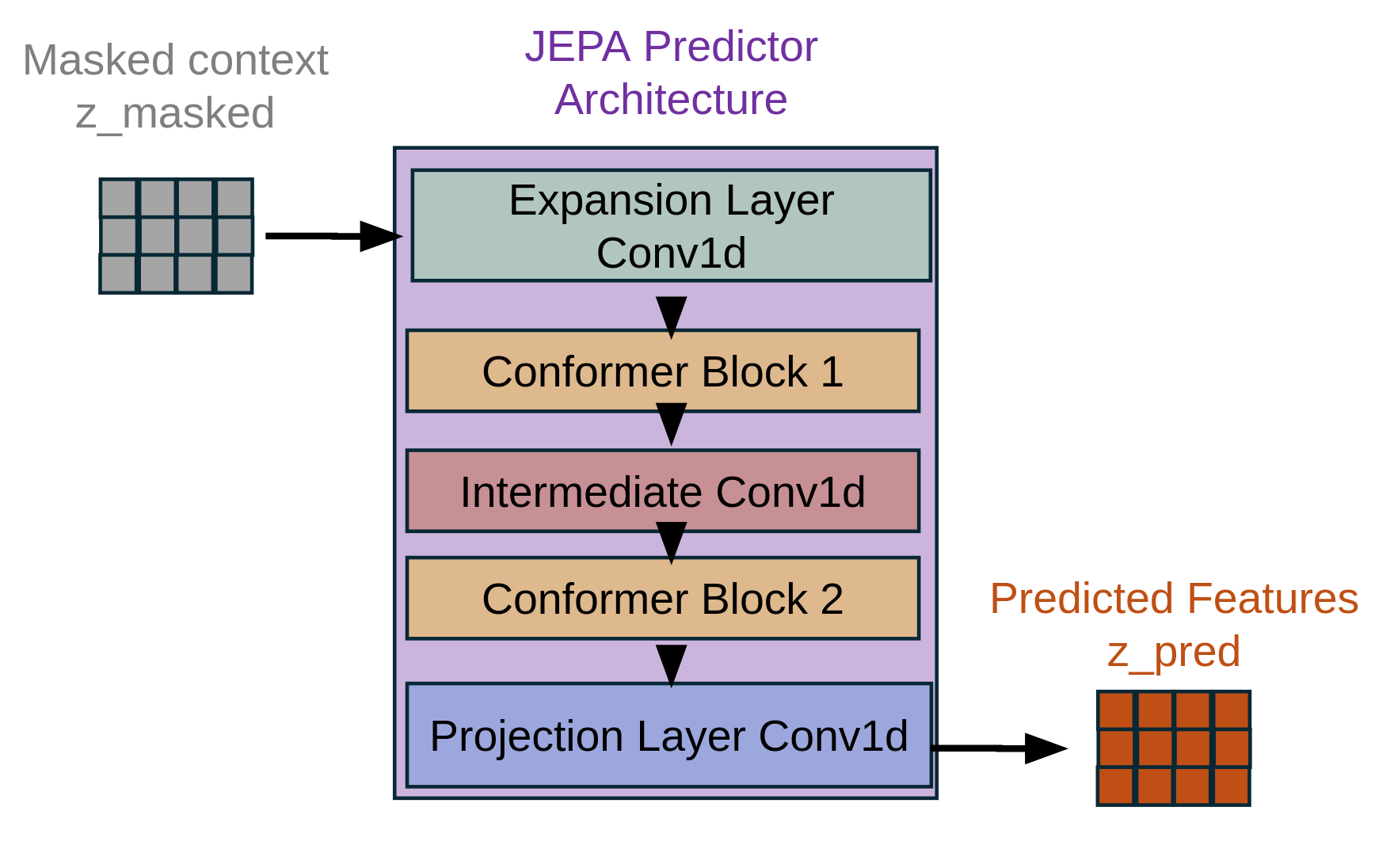
A smaller Conformer predictor receives context features with hidden positions replaced and predicts target features. The loss selects masked positions even though predictions are produced across the sequence. The predictor architecture is preserved in full.
2.5 Stage 1 Training Objective
The first-stage objective is masked latent-feature regression. It is separate from the audio reconstruction and adversarial losses introduced in Stage 2.
2.5.1 Loss Function
Squared prediction errors are averaged over masked positions and feature channels. Gradients do not flow through the target features. This trains agreement with the moving teacher, but agreement alone does not guarantee a useful noncollapsed representation.
Equation 10
| (10) |
2.5.2 EMA Target Update
The target encoder follows an exponential moving average of the online weights. Predictor-output variability is monitored for collapse, but the warning statistic is not itself an anti-collapse loss. The retained training settings distinguish this monitoring from an enforced variance constraint.
Equation 11
| (11) |
3 Stage 2: Fine-Tuning Encoder + FSQ Quantization + HiFi-GAN Decoder
Stage 2 adds discrete scalar quantization and waveform synthesis, while fine-tuning the encoder. The system is therefore reconstruction-free only in its representation-pretraining stage.
3.1 Finite Scalar Quantization (FSQ)
FSQ maps feature coordinates to a fixed set of scalar levels rather than learning a vector codebook. The encoder must adapt so those discretized values retain useful information.
3.1.1 FSQ Formulation
A projection produces quantization coordinates, each clipped and rounded according to its allowed levels. A straight-through gradient approximates differentiation through rounding. These operations discard continuous detail; later integer packing can preserve the resulting discrete indices exactly, but cannot undo that earlier quantization loss.
Equations 12–15
| (12) |
| (13) |
| (14) |
| (15) |
3.2 Mixed-Radix Token Packing
Mixed-radix packing combines several bounded integer indices into one integer token. It is a representation change for already quantized values, allowing a tradeoff between token rate and vocabulary size.
3.2.1 Mixed-Radix Encoding
Each coordinate occupies a place value determined by the product of earlier radices. The preserved example shows how several small indices become one unique integer. Exact decoding requires the same radix order.
Equations 16–18
| (16) |
| token | (17) | |||
| (18) |
3.2.2 Efficient Iterative Computation
Horner-style accumulation computes the packed value using repeated multiply-and-add operations. It avoids materializing a large place-value expansion without changing the mapping.
Equations 19
| (19) |
3.2.3 Padding and Grouping
The quantized dimensions are grouped and padded with radix-one entries when necessary. Nineteen groups per 2.5 Hz frame yield 47.5 tokens per second. Frame rate and token rate describe different levels of the representation.
Equations
3.2.4 Decoding
Repeated integer remainder and division recover the original quantized indices. This exact arithmetic is the reversible part of the pipeline. Waveform reconstruction still depends on a learned decoder.
3.2.5 Comparison to Alternatives
Packing needs no learned codebook and can use integer arithmetic. Its vocabulary grows as the product of group radices, so a lower token rate can require a larger output vocabulary. The comparison table preserves those design differences.
3.2.6 Integration with Language Models
A language model could predict the packed token sequence, followed by unpacking, dequantization and audio decoding. This is an integration route described by the paper rather than a reported end-to-end evaluation of a trained speech language model.
3.2.7 Frame Rate Comparison with Neural Codecs
The codec comparison places frame and token rates side by side. Those rates alone do not compare perceptual quality, bitrate, codebook size or reconstruction error fairly; each system uses a different representation and training recipe.
| Model | Frame Rate | Notes |
|---|---|---|
| Ours (JEPA+FSQ) | 2.5 Hz | Mixed-radix packing (19 groups/frame) |
| U-Codec (Yang and others, 2025) | 5 Hz | Ultra-low for LLM-TTS |
| Mimi (or Multiple, 2025) | 12.5 Hz | Semantic distillation |
| DualCodec (Li et al., 2025) | 12.5–25 Hz | Dual-stream architecture |
| SoundStream (24 kHz) (Zeghidour et al., 2021) | 75 Hz | 13.3 ms frames |
| EnCodec (24 kHz) (Défossez et al., 2022) | 75 Hz | 75 steps/sec @ 24 kHz |
| DAC (44.1 kHz) (Kumar and others, 2024) | 86 Hz | Stride 512 @ 44.1 kHz |
3.3 HiFi-GAN Decoder
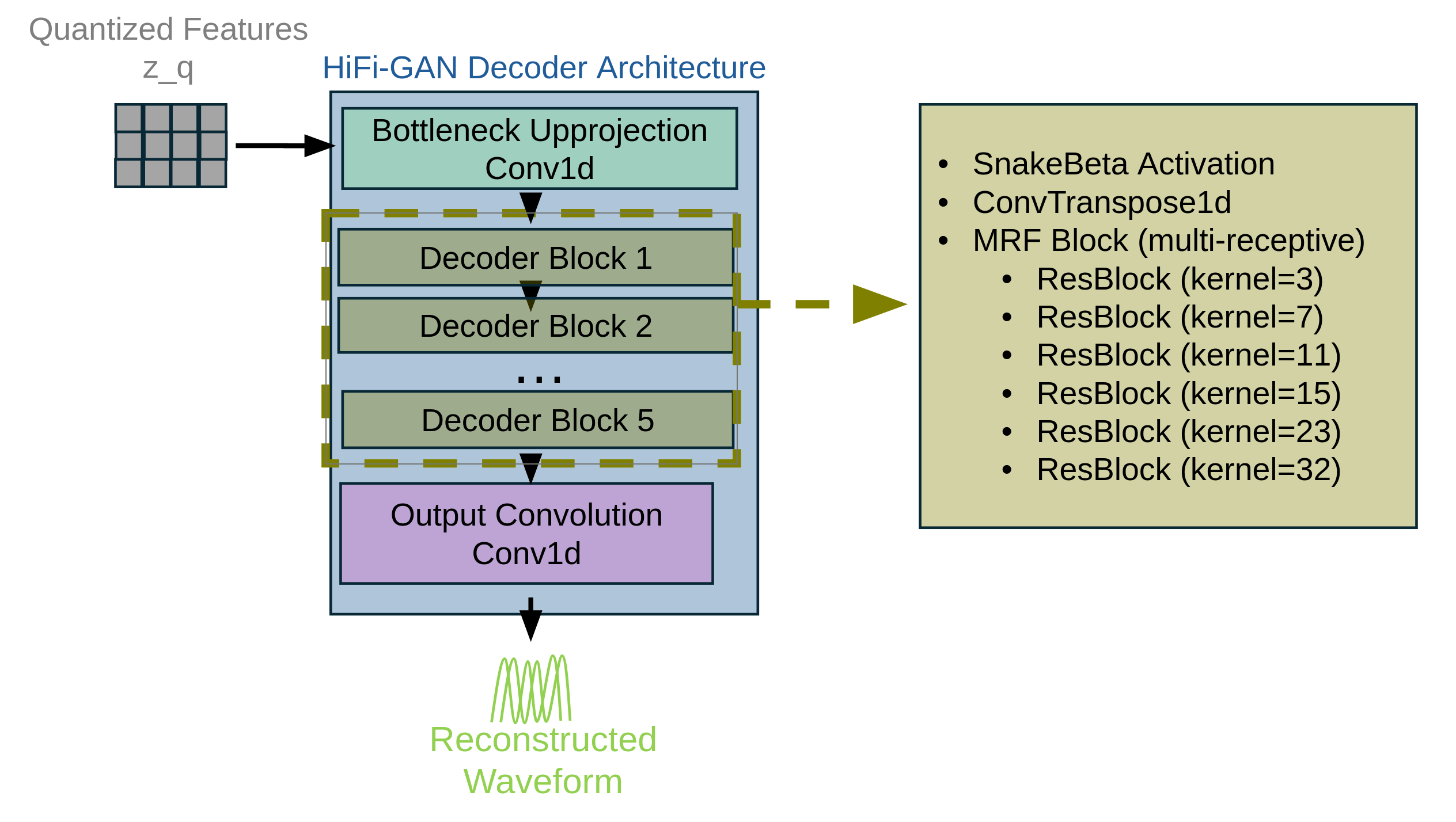
The audio decoder upsamples quantized features into a waveform using a HiFi-GAN-style architecture. Its task differs from the masked latent predictor used during pretraining.
3.3.1 Decoder Architecture
Transposed convolutions restore temporal resolution and residual blocks supply multiple receptive fields. The source includes the full decoder diagram and settings. The output quality depends on both quantized information and decoder learning.
Equation
3.4 Stage 2 Training Objective
The second-stage objective combines waveform fidelity, frequency-domain matching and adversarial learning. It updates the quantizer, decoder and encoder together.
3.4.1 Total Loss
Absolute waveform error encourages sample-level agreement; multi-resolution spectral losses compare frequency structure at several window sizes; adversarial and feature-matching terms promote realistic audio. The discriminator warmup and relative weights affect optimization. A low latent-prediction loss does not by itself establish success on these reconstruction criteria.
Equations 20–28
| (20) |
| (21) |
| (22) |
| (23) |
| (24) |
| (25) |
| (26) |
| (27) |
| (28) |
4 Experimental Setup
The experimental setup specifies the speech corpus, preprocessing, hardware and inference sequence. These details bound the scale and reproducibility of the preliminary study.
4.1 Dataset
Training uses unlabeled English speech from LibriLight and holds out speakers for validation. Sample rate, clip length and corpus size constrain what acoustic variation the model sees.
4.2 Data Preprocessing
Audio is resampled to 24 kHz and converted to mono. In-model normalization handles remaining amplitude processing. This preprocessing does not by itself establish robustness to multilingual or noisy deployment audio.
4.3 Distributed Training
The reported run uses two A 100 GPUs and mixed precision, with critical operations in higher precision. Global batch size differs between stages, so their step counts should not be compared as identical amounts of training exposure.
4.4 Inference Pipeline
Inference follows encoder, quantizer, token packing/unpacking and waveform decoder. The target encoder and training-only prediction branch are not required. The stated token rate describes the discrete interface, not a directly measured lossless audio bitrate.
5 Model Architecture and Efficiency
The efficiency section counts the model components and reports the two-stage training setup. It should be read alongside the limited evaluation evidence.
5.1 Parameter Counts
The parameter table distinguishes encoder, predictor, target and decoder components. Inference can omit training-only branches, but the complete reconstruction system still includes its decoder.
| Component | Parameters | Notes |
|---|---|---|
| Stage 1: JEPA encoder training | ||
| Online encoder | 121.7M | Trainable |
| Target encoder (EMA) | 118.5M | Momentum update |
| Predictor network | 3.2M | Trainable |
| Stage 1 total | 240.2M | 121.7M trainable |
| Stage 2: decoder training | ||
| JEPA encoder | 240.2M | Fine-tuned |
| FSQ quantizer | M | Trainable |
| HiFi-GAN decoder | 69.2M | Trainable |
| Stage 2 total | 309.5M | 69.3M trainable |
| Final model (inference) | ||
| Encoder only | 121.7M | Online encoder only |
| FSQ + decoder | 69.3M | |
| Inference total | 191.0M | Single-pass model |
5.2 Training Efficiency
Pretraining supplies an initialization for reconstruction-focused fine-tuning. The reported inference parameter count excludes the EMA branch. This architectural accounting is different from a controlled wall-clock or perceptual-quality comparison against every codec baseline.
| Metric | Stage 1 (JEPA) | Stage 2 (decoder) |
|---|---|---|
| Trainable parameters | 121.7M (50.7%) | 69.3M (22.4%) |
| Training steps | 24K | 29K |
| Batch size | 32 | 8 |
| Learning rate |
6 Evaluation Metrics
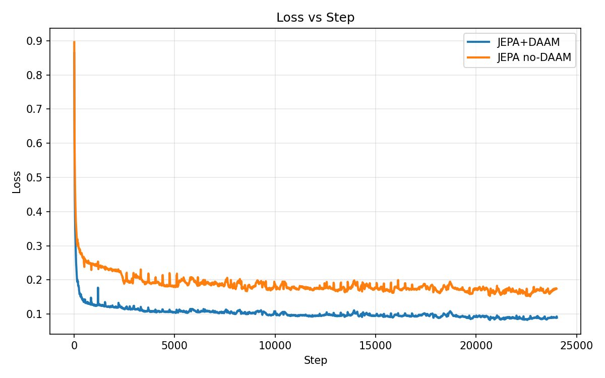
The authors explicitly describe the evaluation as qualitative and preliminary under a limited compute budget. The shown latent-loss curve compares training behavior, not a standardized speech-understanding or reconstruction-quality benchmark. Broad claims of codec competitiveness should be interpreted with that limitation.
7 Discussion
The discussion interprets density gating as a different way to choose informative temporal features. Those mechanisms remain hypotheses to test quantitatively.
7.1 Why DAAM Improves JEPA Representations
Pairwise attention models relationships between positions; density-based gating modulates features using learned temporal statistics. Avoiding a full pairwise gate can be cheaper, but it does not remove the cost of the Conformer attention elsewhere in the architecture.
8 Limitations and Future Work
The stated limits include fixed masking, English-only experiments and modest training scale. Multilingual, cross-modal and broader downstream evaluations remain future work. These boundaries are essential when considering the model as a general-purpose speech tokenizer.
9 Code Availability
The source links the training and model implementation, including quantization, token packing and audio decoding. Reproducing the exact gate placement and schedules requires following that version’s code as well as the narrative.
10 Conclusion
The contribution is a concrete staged design: latent prediction with density gates, followed by quantized reconstruction. The integer packing preserves discrete indices exactly; the full speech codec remains learned and lossy. Stronger quantitative evaluations are needed before treating the preliminary results as a general replacement for established neural codecs.