Overview
SIMPACT builds a task-specific simulator from a calibrated RGB-D observation, then uses simulated outcomes to refine vision–language-model action proposals. The supplementary material details prompts, physical-parameter estimates, timing, failures, and optional replanning.
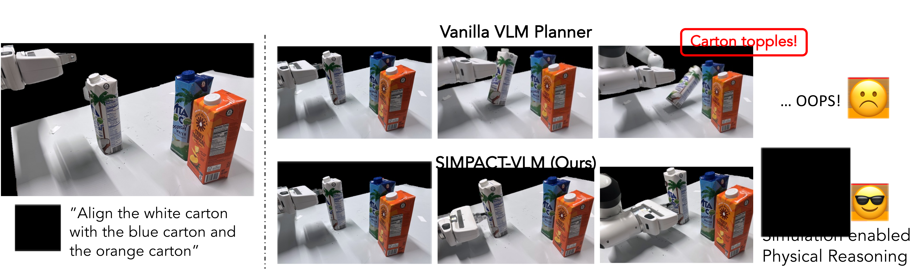
At a glance
Without additional model training, SIMPACT combines pretrained perception and vision–language models with rigid or deformable simulation. A model proposes parameterized symbolic actions, reviews simulated trajectories, and refines a plan before physical execution. Seven real manipulation tasks show 40–90% success over ten trials each. Results rely on a calibrated setup, specified action primitives, inferred physical properties, and minutes of planning; main execution is open-loop, with limited recovery experiments reported separately.
1 Introduction
Semantic task descriptions alone can miss consequences of contact, friction, and deformation. SIMPACT adds a constructed physics model so proposed actions have predicted outcomes that a vision–language model can inspect. The contribution combines single-view scene reconstruction with a test-time sampling/refinement loop, using pretrained components rather than new task-specific training. The resulting physical reasoning remains dependent on reconstruction and simulation accuracy.
2 Related Works
Spatially grounded language planners use value maps, keypoints, affordances, or constraints, while model-based controllers evaluate predicted dynamics. SIMPACT combines these ideas with automatic scene construction and multiple physics engines. Unlike the compared Prompting-with-the-Future method [45], it uses the language model for action proposals and refinement as well as outcome evaluation. Comparisons concern these particular implementations and tasks, not a universal ranking of all model-based or learned policies.
3 Method
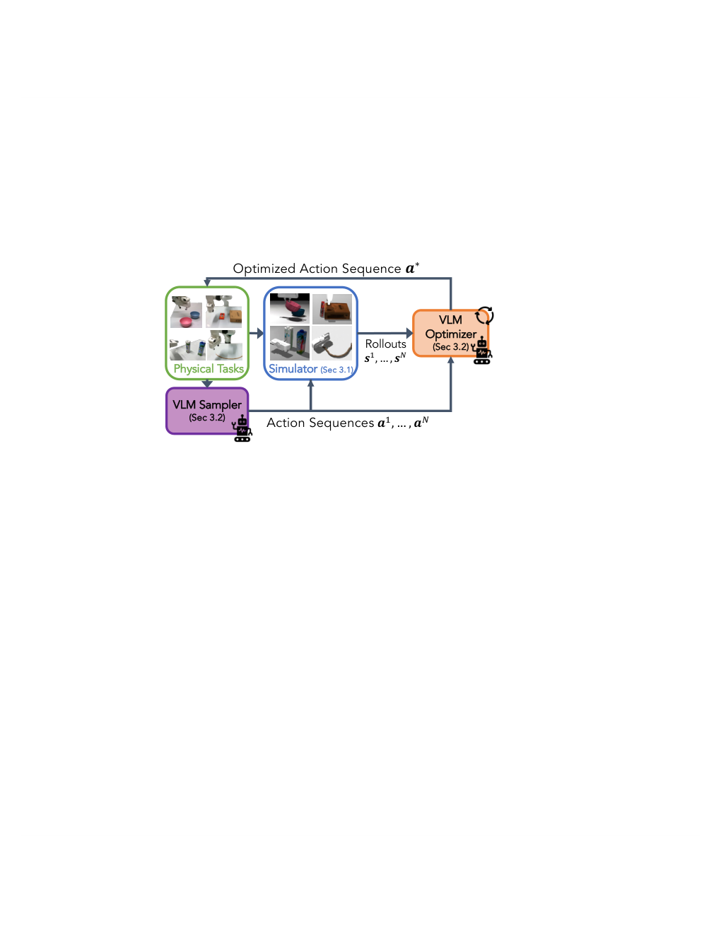
The input includes a task instruction with requirements and possible success/failure conditions, calibrated RGB-D data, robot state, and reconstructed object properties. Planning constructs a simulator, generates candidates, rolls them out, and asks the model to improve them from visual and numerical context. The final sequence becomes end-effector pose/gripper commands. Simulation-loop feedback occurs before execution; the principal physical policy does not continuously replan during contact.
3.1 Simulation Construction
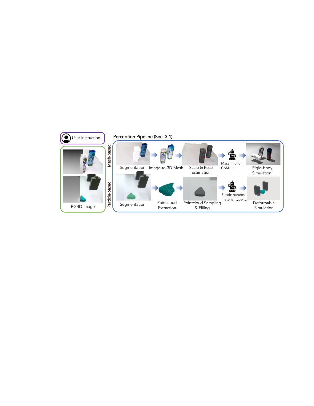
The simulator state contains rigid poses or deformable particle positions, with geometry and mechanical parameters inferred from the initial observation. GroundedSAM2 [55] segments task-relevant objects. The model selects MuJoCo for rigid objects, a projective-dynamics variant for stiff deformables, or a material-point solver for soft materials. Objects are assumed static before interaction. Material guesses are commonsense priors, not measurements obtained through system identification.
Equation 1
| (1) |
Mesh-based Rigid Body Simulation.
For rigid objects, Hunyuan3D [57] generates a complete mesh from the segmented image. The mesh is centered and scaled using the observed point-cloud bounding box, then aligned with FoundationPose [63]. Mass, friction, and center of mass enter the physics model. Single-view occlusions and reconstructed unseen geometry can therefore affect contact planning.
Particle-based Deformable Object Simulation.
For deformables, segmented depth yields visible surface points. Particles fill the volume between that surface and the supporting table. Elasticity and plasticity parameters configure deformation. This construction is suited to the tested supported objects, without demonstrating arbitrary hidden geometry, articulated mechanisms, or unrestricted material identification.
3.2 Action Planning via Simulation-enabled VLM
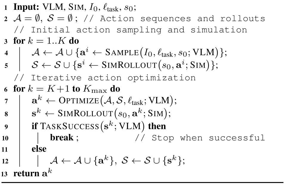
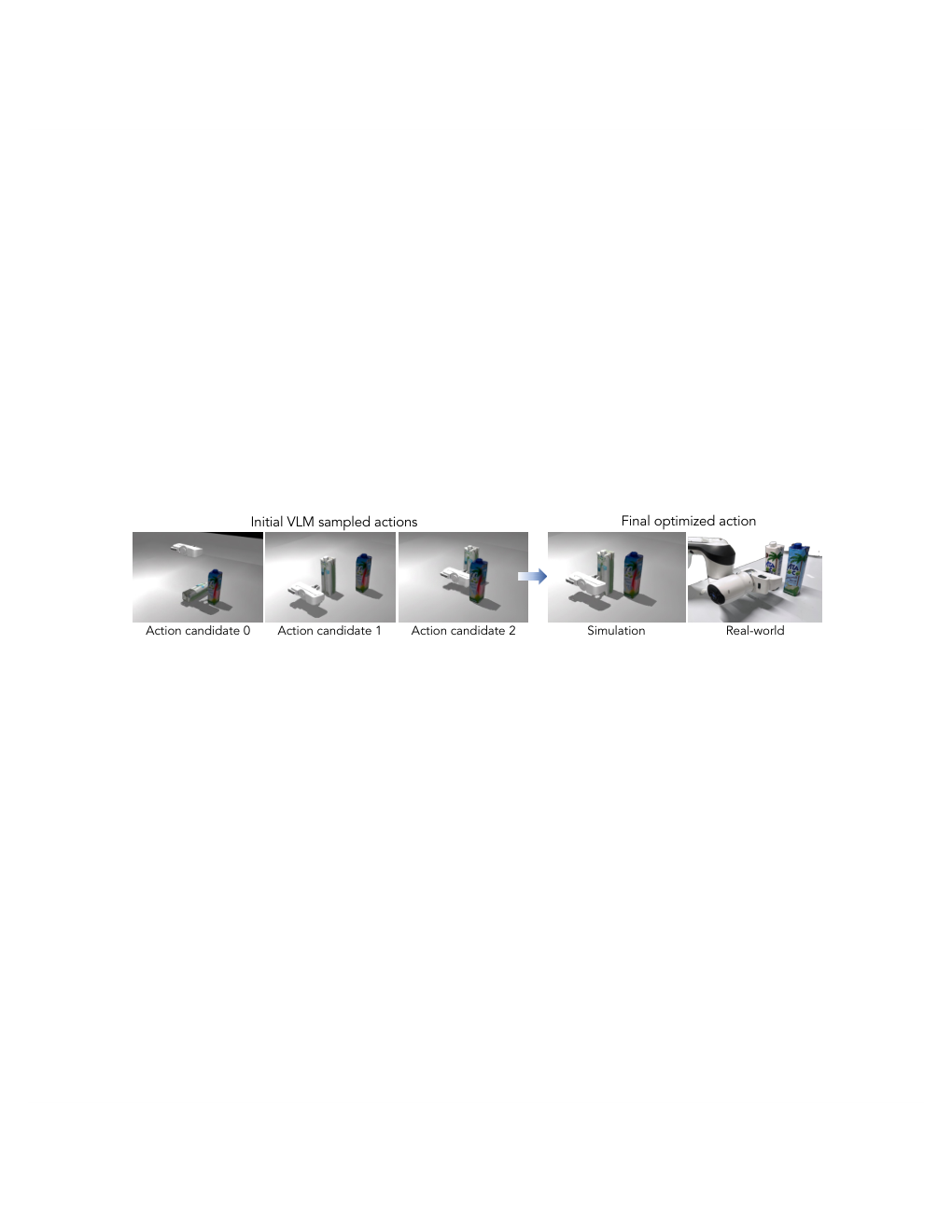
The default model supplies ten initial candidates and up to three refinement iterations. Each new candidate is simulated and evaluated using its final image and state; failed attempts are retained as context. The prose describes executing a verified successful plan, but the original pseudocode returns the last candidate when its iteration limit is reached without an explicit failure flag. A simulation verdict therefore should not be interpreted as a formal execution guarantee.
| Tasks | Instruction | Success Condition |
| Non-toppling push | Push the white carton forward to align horizontally with the others. | The bottle does not topple and aligns within 2 cm. |
| Bowl stacking | Grasp the pink bowl at its edge and stack it with the blue bowl. | The pink bowl stably lies inside the blue bowl. |
| Pivoting | Make the red pocky box lean vertically against the brown box. | The red pocky box reaches vertical pose. |
| Shape rope | Grab the free end of the rope and arrange the rope to a U shape. | The deformed rope has an opening ratio in . |
| Shape playdoh | Squeeze the Play-Doh to a square shape with equal sides. | Two sides of the Play-Doh have a ratio within 1.5. |
| Avoid obstacle | Push the orange bottle around the box to the image’s bottom-right. | The orange bottle reaches the other side without colliding. |
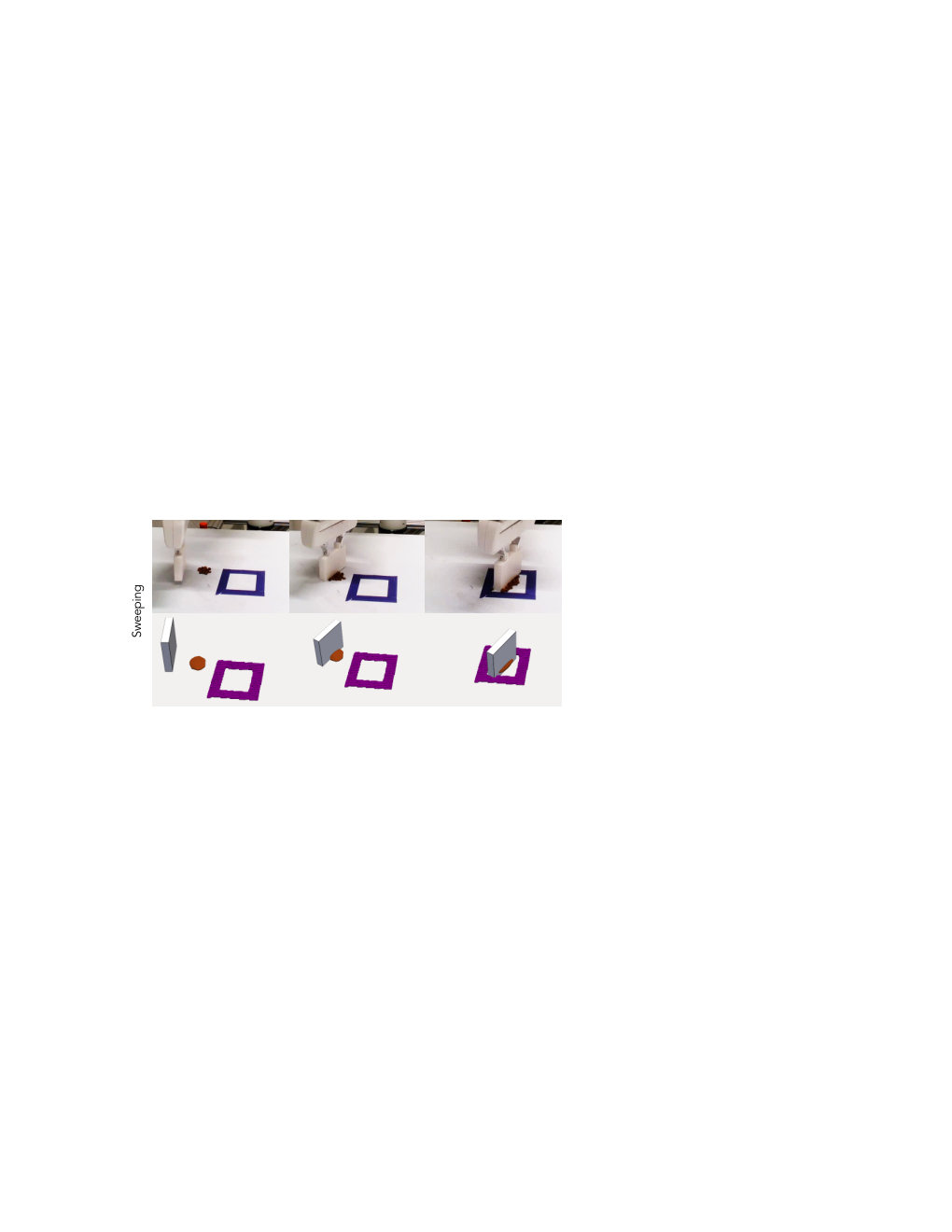
| Sweeping | Sweep the coffee beans into the purple box. | All beans are pushed into the box. |
VLMs for Action Proposal Generation.
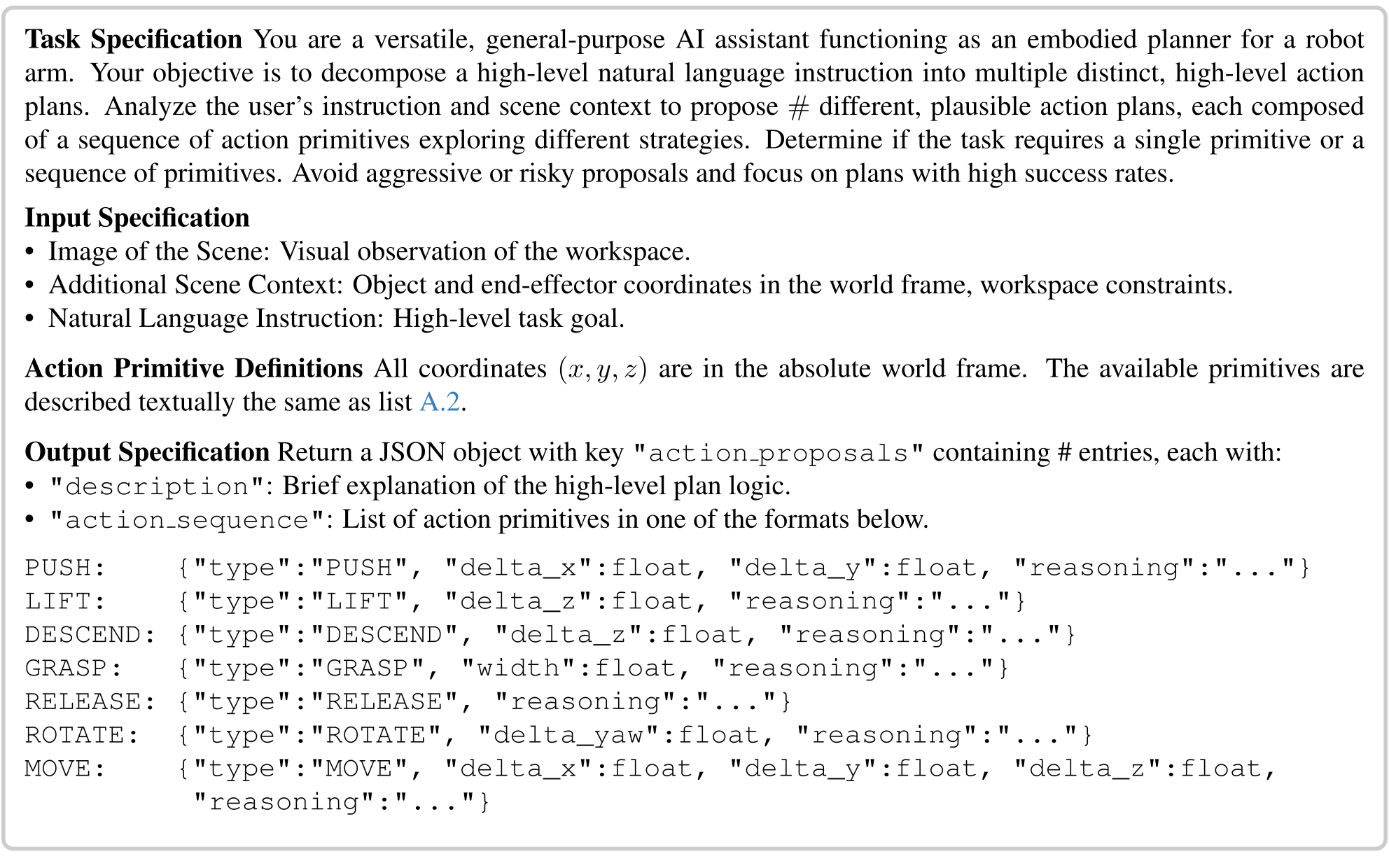
Action proposals use the initial image, robot pose, object poses and dimensions, task goal, and workspace context. Symbolic primitives such as push, lift, grasp, release, rotate, and move carry continuous offsets or gripper width. A deterministic mapping converts them to pose trajectories. This constrained interface gives the model meaningful choices but bounds the behaviors it can express.
Equation
VLMs for Action Optimization.
The optimizer receives candidate actions plus rendered states and numerical object/gripper information at action boundaries. It can change the strategy rather than only perturb nearby numerical parameters. Example updates lower a pushing contact to avoid toppling and adjust travel distance. This is in-context inference over simulated attempts, not parameter learning or an optimization-convergence proof.
Equation 2
| (2) |
VLMs for Success Evaluation.
A model checks final simulated images and state against task requirements. Negative judgments trigger further refinement within the budget. Errors in the simulator or evaluator can still pass a plan that fails physically; the separate sim–real analysis quantifies such discrepancies for a limited sample.
Equation
| Method | Non-toppling push | Bowl stacking | Pivoting | Shape rope | Shape dough | Avoid obstacle | Sweeping |
| [2] | 0% | 0% | 0% | 0% | 0% | 0% | 0% |
| VoxPoser[26] | 0% | 20% | 0% | 0% | 0% | 0% | 20% |
| MOKA[16] | 0% | 10% | 0% | 20% | 0% | 0% | 0% |
| Ours | 80% | 60% | 40% | 90% | 80% | 80% | 70% |
4 Experiments
Seven custom physical tasks cover rigid contact, stacking, pivoting, rope shaping, dough shaping, obstacle avoidance, and sweeping. Main comparisons use ten trials per task/method, a small sample with ten-percentage-point resolution.
4.1 Experimental Setup
Hardware is a Franka Research 3 with parallel jaws and one calibrated RealSense D435i camera. Dough manipulation uses a custom printed end effector for broader contact. These embodiment and calibration choices are part of the tested system.
Tasks and Metrics.
Task success uses explicit geometric or completion conditions: carton alignment within two centimeters without toppling, stable nested bowls, a vertically leaning box, rope opening ratio between 0.5 and 2.0, dough side ratio within 1.5, collision-free passage around a box, and every bean swept into its container. The dough criterion permits approximate squareness; it is not exact shape reconstruction.
| Method | Non-toppling push | Bowl stacking | Pivoting | Shape rope | Shape dough | Avoid obstacle | Sweeping |
| w/o VLM sampler | 0% | 10% | 0% | 0% | 0% | 0% | 20% |
| w/o simulation rollout | 20% | 0% | 0% | 30% | 30% | 0% | 20% |
| w/o VLM optimizer | 30% | 50% | 30% | 40% | 80% | 20% | 70% |
| Ours | 80% | 60% | 40% | 90% | 80% | 80% | 70% |
Baselines.
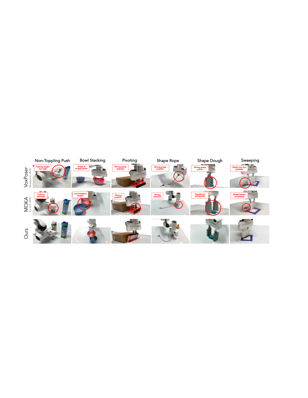
Baselines are the pretrained π0.5 policy, VoxPoser’s volumetric affordance planner, and MOKA’s keypoint/affordance planner. MOKA is extended to pushing and squeezing via contact points and directions. These are out-of-domain zero-shot challenges for the baselines, so poor performance does not establish their general inability to perform manipulation.
Implementation details.
Gemini 2.5 Pro supplies proposals, refinement, and evaluation. The stiff-deformable solver is implemented in PyTorch and the material-point solver in Warp. Ten initial proposals plus at most three optimized proposals set the default planning budget.
4.2 Results
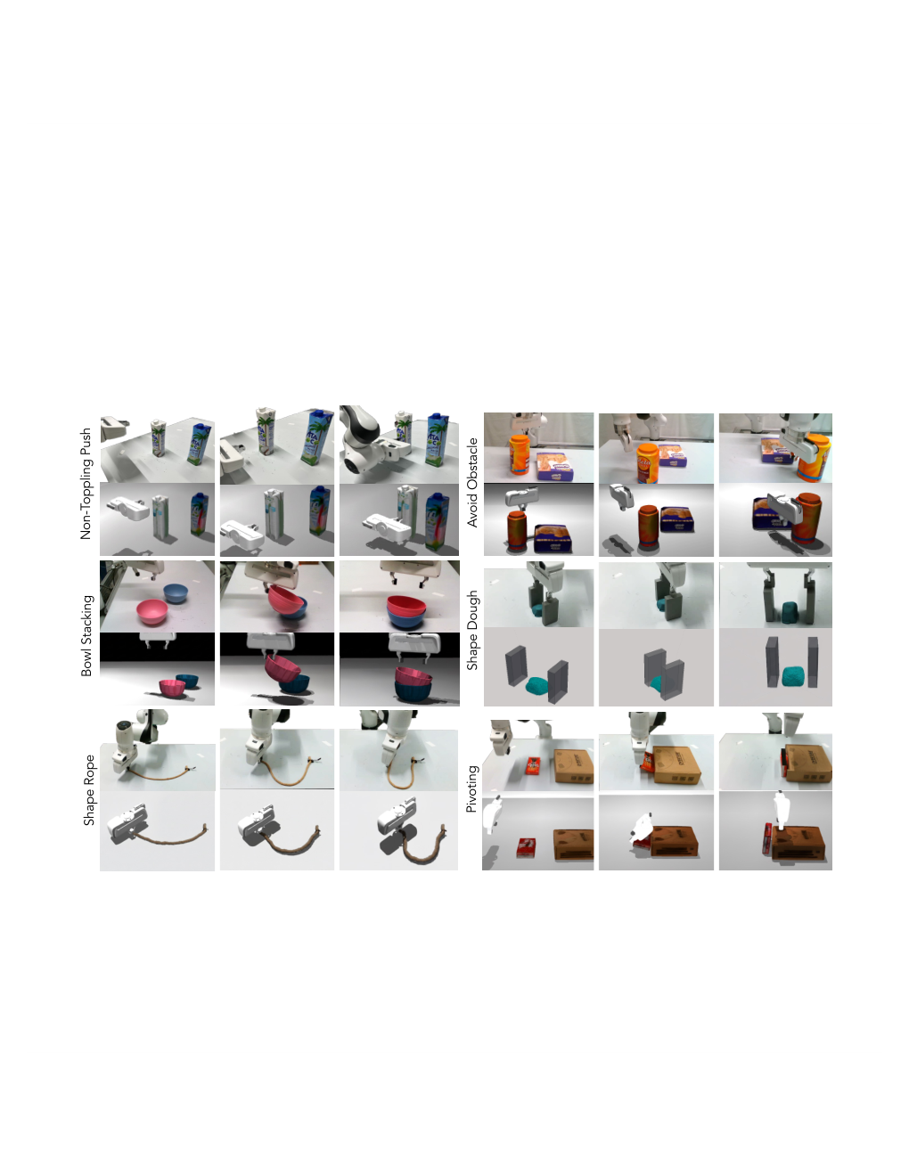
Success is 80% non-toppling push, 60% bowl stacking, 40% pivoting, 90% rope shaping, 80% dough shaping, 80% obstacle avoidance, and 70% sweeping. That is fifty successes across seventy task trials. π0.5 records zero in these tests; VoxPoser and MOKA achieve isolated 10–20% results. Simulated and physical rollout panels illustrate the contact strategies, while pivoting remains the weakest SIMPACT task.
4.3 Ablation study
Removing informed sampling is damaging despite five times as many random proposals. Removing simulation context also lowers success. Refinement helps most on pushing, rope shaping, and obstacle avoidance, but dough and sweeping tie the no-optimizer variant at 80% and 70%. More proposals are not always better: increasing ten to twenty improves pushing from 80% to 90%, but reduces stacking from 60% to 20% and rope shaping from 90% to 80%. Context overload is the authors’ explanation, not an independently isolated cause.
| #Samples | Non-toppling push | Bowl stacking | Shape rope |
| 3 samples | 50% | 50% | 40% |
| 10 samples | 80% | 60% | 90% |
| 20 samples | 90% | 20% | 80% |
4.4 Failure Case Analysis
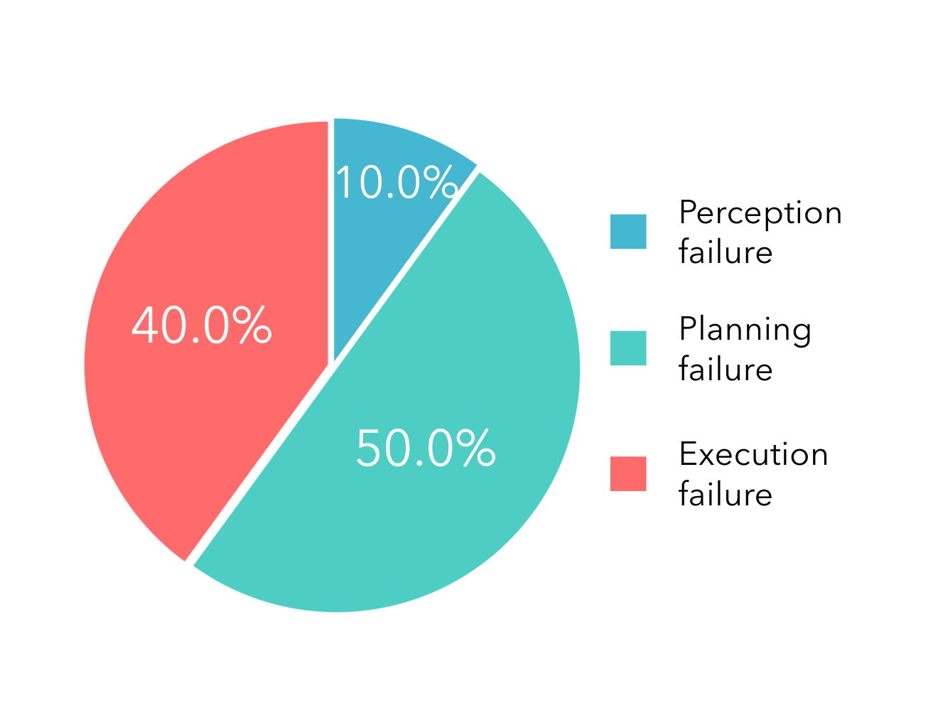
Failures are grouped into perception, planning, and execution. Single-view reconstruction can give wrong geometry; refinement can fail to locate a feasible contact strategy; and simulated success can fail on hardware because of pose or dynamics errors. Planning is the largest reported category, particularly for pivoting.
4.5 Limitations
The system depends on single-view geometry, commonsense material estimates, and open-loop physical execution. Occlusion and parameter errors create sim–real gaps, while small execution offsets can compound. Proposed improvements include better completion/reconstruction, articulated models, interaction-based parameter identification, and tighter feedback. Optional recovery updates the simulator after failure, but is tested only on two tasks.
5 Conclusion
Simulation-informed proposal refinement improves this set of carefully specified physical tasks without task-specific model training. The evidence supports the tested integration of perception, physics, and language inference; it does not demonstrate universal scene understanding, real-time control, or guaranteed contact accuracy.
Acknowledgements
The acknowledgments credit help with experimental design, hardware, real-to-simulation implementation, and MOKA, and list support from the Kempner Institute, Amazon, and Pickle Robot.
Appendix A Implementation Details
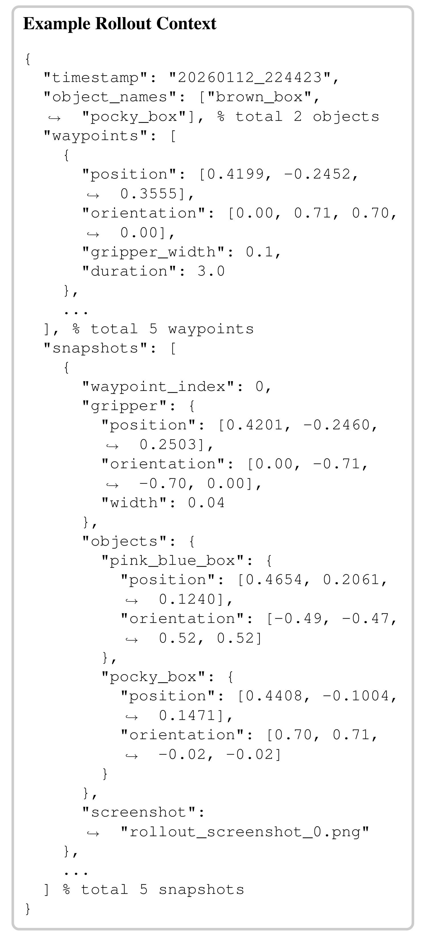
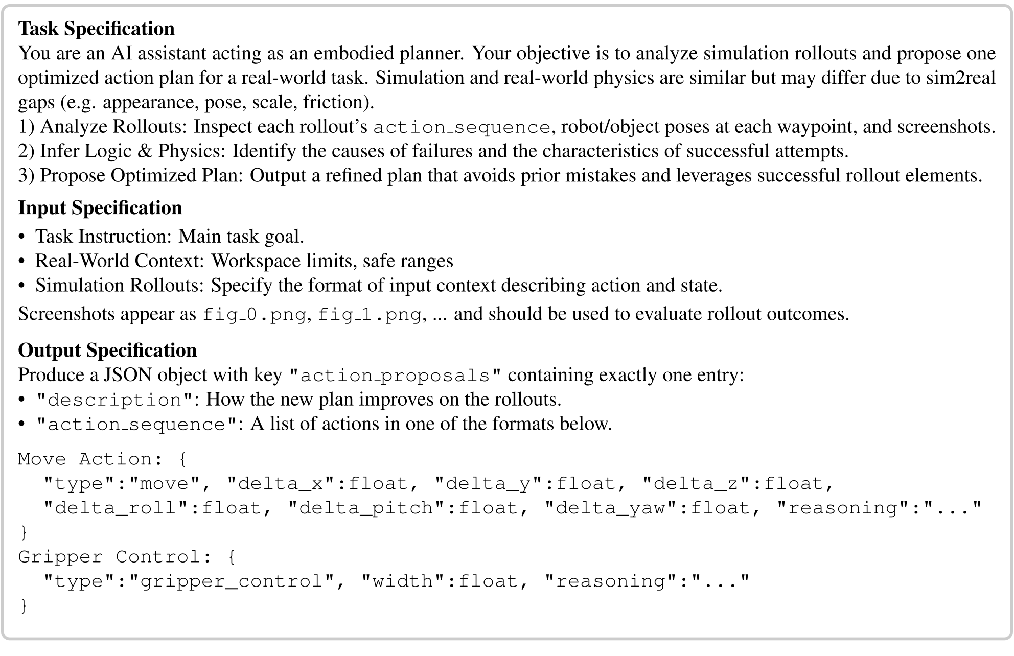
The implementation appendix gives material-parameter questions, the complete symbolic action definitions, and sampling/refinement prompts with an example rollout context. All original prompt text and code formatting are retained.
A.1 Simulation Construction Details
Simulation setup selects a physics model and queries plausible parameters from the scene and object description. The original five-question sequence is preserved as a separate reading block.
Physical Parameters θ phys Prediction
Questions first identify manipulated objects and choose rigid or deformable simulation. Rigid objects receive mass and friction estimates. Stiff deformables use Young’s modulus, Poisson’s ratio, and density; material-point objects additionally select among jelly, metal, sand, foam, and plasticine, with friction angle or yield stress when applicable. These predictions provide simulator defaults rather than experimentally calibrated ground truth.
Identify the objects that need to be manipulated from {task instruction}. Determine whether to use a rigid or deformable object simulator based on the object’s material.
For rigid {object}, predict its mass and friction parameters.
For deformable {object}, decide whether to use Projective Dynamics or the Material Point Method based on the stiffness of the object.
For {object} simulated with Projective Dynamics, determine the following physical parameters:
-
Young’s modulus
-
Poisson’s ratio
-
Mass density
For {object} simulated with the Material Point Method, first determine the material type of {object} from the set: {jelly, metal, sand, foam, plasticine}. Then output:
-
Young’s modulus
-
Poisson’s ratio
-
Mass density
-
(Optional) Friction angle
-
(Optional) Yield stress
A.2 Action Planning Details
Seven primitives define horizontal push, vertical lift/descent, gripper width, release, yaw rotation, and three-dimensional displacement. End-of-primitive snapshots include rigid transforms or downsampled deformable keypoints/bounds. The source prompts and JSON-like examples remain exact, including their differing sampler/optimizer schemas, absolute-coordinate wording alongside delta fields, example object-name inconsistency, and abbreviated comments. These are published prompt outlines, not a fully executable validated interchange specification.
-
PUSH(, ): Move the end-effector horizontally from its current position by while maintaining its current height.
-
LIFT(): Move the end-effector upwards along the -axis by .
-
DESCEND(): Move the end-effector downwards along the -axis by .
-
GRASP(): Adjust gripper to a target width (in meters), where is fully closed and is fully open.
-
RELEASE: Fully open the gripper.
-
ROTATE(): Adjust end-effector yaw relative to its current orientation by (in radians).
-
MOVE(, , ): Move the end-effector from current position by (, , ).
Appendix B Supplementary Results
Supplementary tests cover sweeping, sampling-based optimization, sim–real outcome agreement, computation time, scene variation, parameter sensitivity, CALVIN, failure examples, and recovery.
B.1 Additional Qualitative Results
The extra sweeping panel supplies the seventh task’s simulated and physical sequence, complementing the six tasks shown in the main rollout figure.
B.2 Further Ablation Analysis
A random-sampling/CEM variant uses the model only to judge outcomes and reports zero success on these tasks. It follows the referenced method’s released optimizer/hyperparameters. This supports informed proposals and refinement in this action/task setup, without invalidating the original method’s results on its own pick-and-place domain.
B.3 Correlation Between Simulation and Real-World Performance
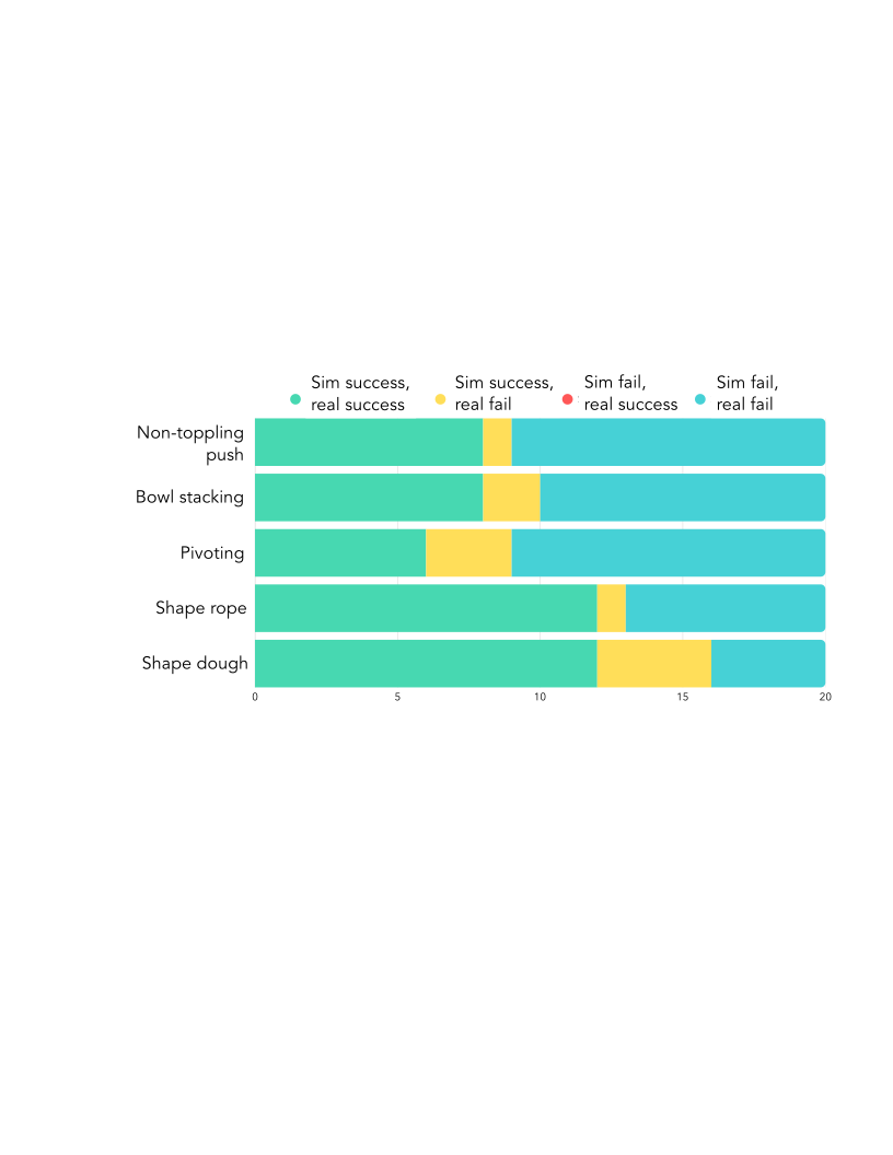
Five tasks contribute twenty sequences each: ten optimized plans and ten raw proposals. Simulation and reality agree on eighty-nine of these hundred outcomes; eleven are simulated successes that fail physically, and none fail only in simulation. This is outcome agreement on a deliberately mixed sample, not 89% task success or calibrated physical prediction over arbitrary actions. Pivoting and dough have 15% and 20% false-success discrepancy among their twenty samples.
B.4 Computation Time
Mean component times are 1.9 minutes for simulator construction, 2.8 for action sampling, 0.8 for rollouts, and 0.9 for optimization—about 6.4 minutes when summed. Model inference and network calls dominate. Individual simulations take five to eight seconds. The system is a minutes-scale pre-execution planner in this implementation, not a low-latency feedback controller.
| Component | Time (mins) |
| simulation construction | 1.9 |
| action sampling | 2.8 |
| simulation rollout | 0.8 |
| action optimization | 0.9 |
B.5 Robustness Validation
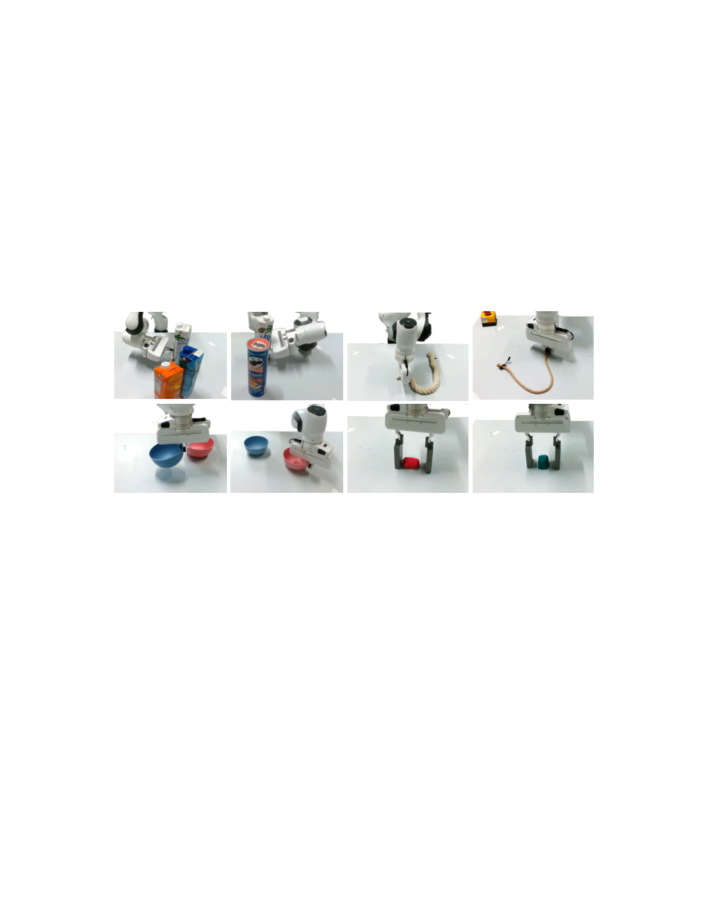
Illustrations vary distractors, relative poses, object appearance, and materials. They show the kinds of scene changes included in evaluation, but do not provide a large separate robustness benchmark or isolate each variation’s effect.
B.6 Physics Parameters Estimation Analysis
Ten repeated material predictions are summarized, and a friction sweep probes downstream sensitivity. Estimated consistency does not establish parameter accuracy. Some reported standard deviations are incompatible with their stated ten-sample ranges, so Table 6 should be treated cautiously rather than silently corrected. Friction values 0.01/0.20/0.50/1.00/10.0 produce 40/100/80/80/0% success. This limited sweep supports sensitivity at extreme values, not universal robustness of inferred physics.
| Task | Parameter | Mean Std | Range [Min, Max] |
| Non-toppling Push | Mass (kg) | ||
| Friction Coeff. | |||
| Shape Playdoh | Poisson’s Ratio | ||
| Mass Density (kg/m3) |
| Fric. Coeff. () | 0.01 | 0.20 | 0.50 | 1.00 | 10.0 |
| Success Rate (%) | 40 | 100 | 80 | 80 | 0 |
B.7 Standardized Benchmark Results
CALVIN evaluation uses forty instruction chains and ground-truth segmentation masks. SIMPACT averages 2.78 completed instructions, above HULC’s 0.67 and RoboFlamingo’s 2.47 but below FLOWER’s 4.53 [56]. Its five-instruction completion is 20.0%, below RoboFlamingo’s 23.5%, despite the higher average length. Privileged masks, the small sample, and differing trained-versus-zero-shot conditions qualify this benchmark comparison.
| #. Instruct. | zero-shot | 1 | 2 | 3 | 4 | 5 | Avg. Len. |
| HULC [40] | ✗ | 41.8% | 16.5% | 5.7% | 1.9% | 1.1% | 0.67 |
| RoboFlamingo [35] | ✗ | 82.4% | 61.9% | 46.6% | 33.1% | 23.5% | 2.47 |
| FLOWER [56] | ✗ | 99.4% | 95.8% | 90.7% | 84.9% | 77.8% | 4.53 |
| Ours | ✓ | 87.5% | 82.5% | 47.5% | 40.0% | 20.0% | 2.78 |
B.8 Failure Cases
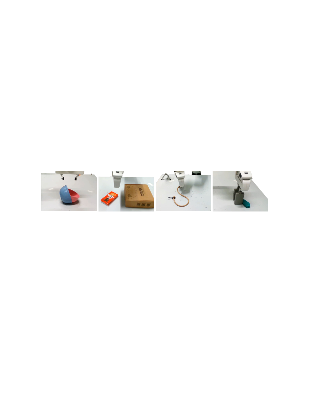
Examples show bowl-placement flips and failed dough squeezes after small execution offsets. Pivoting can miss a narrow stable contact range, and rope proposals can lack sufficient diversity. Increasing proposal count is only a possible remedy; the main count ablation also shows degradation when context grows.
B.9 Replanning using Real-world Feedback.
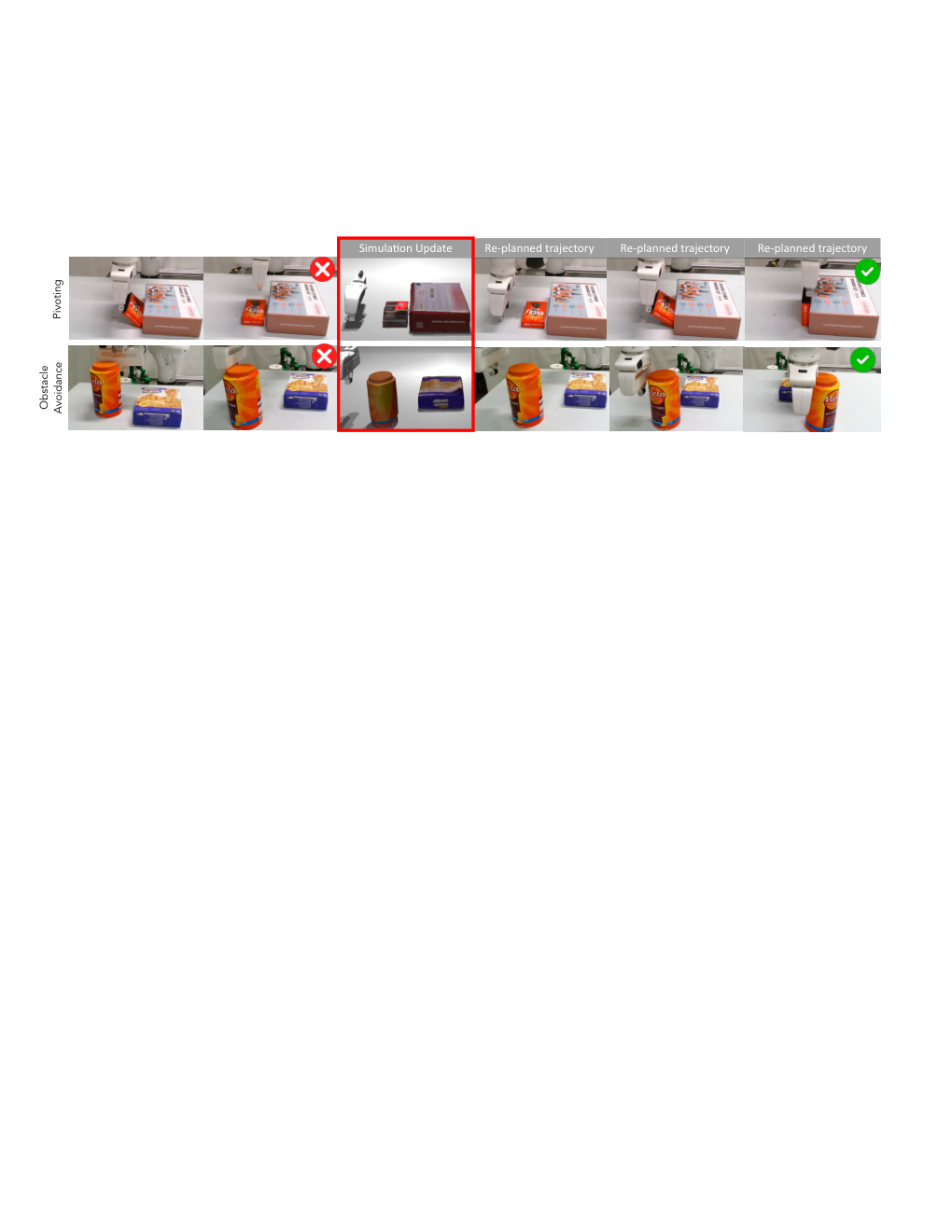
Optional recovery updates the simulator from the new physical state and allows up to three replanning attempts. It recovers three of six initial pivoting failures and both of two obstacle-avoidance failures, with mean attempts 1.67 and 1.0 among the reported recoveries. These small conditional tests support recovery feasibility rather than a general closed-loop success guarantee.