At a glance
A simple active-learning pipeline splits a colored point cloud into vertical columns and requests labels for columns with high ensemble uncertainty. Experiments compare region partitions and query rules on S3DIS, Toronto-3D and partially annotated Freiburg data. Small columns with ensemble entropy or vote disagreement are competitive with more elaborate heuristics, while requiring much less preprocessing. An area-based annotation-cost proxy exposes differences hidden by labeled-point counts; it is not a direct measurement of annotation time.
I Introduction
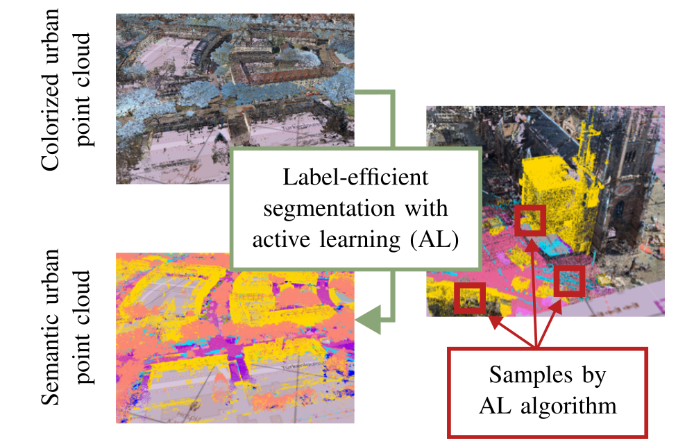
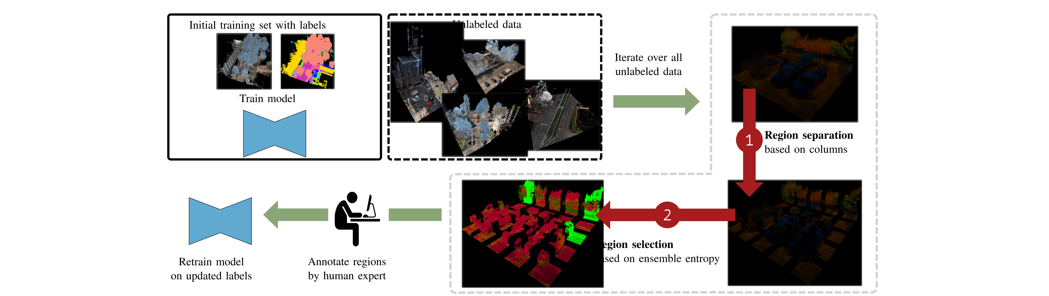
City-scale segmentation supports environmental modeling, but drawing 3D labels is expensive. Active learning alternates model training, region selection and annotation. Two decisions matter separately: how to partition the cloud into human-manageable regions, and which regions to label next. The proposal replaces geometry/color clustering heuristics with an XY grid and a four-model ensemble.
This edition follows all nine pages of arXiv v1, dated 5 December 2025. The empirical claims concern segmentation and annotation proxies; the paper does not evaluate downstream climate simulations or establish measured human-time savings against every competing pipeline.
II Related Work
Sparse scribbles and pretrained image models offer other routes to reducing labels. This study focuses on region-based active learning, where a query requests labels for an entire selected portion of the point cloud.
II-A Active Learning
Query policies may emphasize diversity, uncertainty or expected model change. Diversity can select unusual but unhelpful samples, while a single network’s softmax confidence can be poorly calibrated. The active-learning survey motivates hybrid strategies; here the authors test whether ensemble uncertainty alone can compete with task-specific hybrids.
II-B Active Learning for Point Cloud Segmentation
ReDAL combines supervoxels, entropy, color/surface heuristics and feature-cluster diversity. SSDR-AL uses uncertainty/class-balancing proposals followed by diversity-space sampling. Samet et al. show that the initial labeled set matters, using image-model features for seeding. Pointwise queries can need few labels yet touch many scattered objects, motivating explicit attention to the spatial extent of annotation.
III Approach
Keep partitioning and ranking separate: the first defines annotation units, the second assigns an information score. This makes it possible to test a simple partition with an existing query rule before changing both components.
III-A Region Separation
The main comparison is between fixed vertical columns and geometry-dependent supervoxels. Neither guarantees that a region corresponds to one semantic object.
III-A 1 Columns
Place a grid of edge length r on the XY plane and assign all points above each cell to one column. Regions can be specified by grid coordinates instead of stored index clusters. Resolution controls spatial granularity; fixed XY area does not impose a uniform point count or annotation time when height and density vary.
III-A 2 Supervoxels
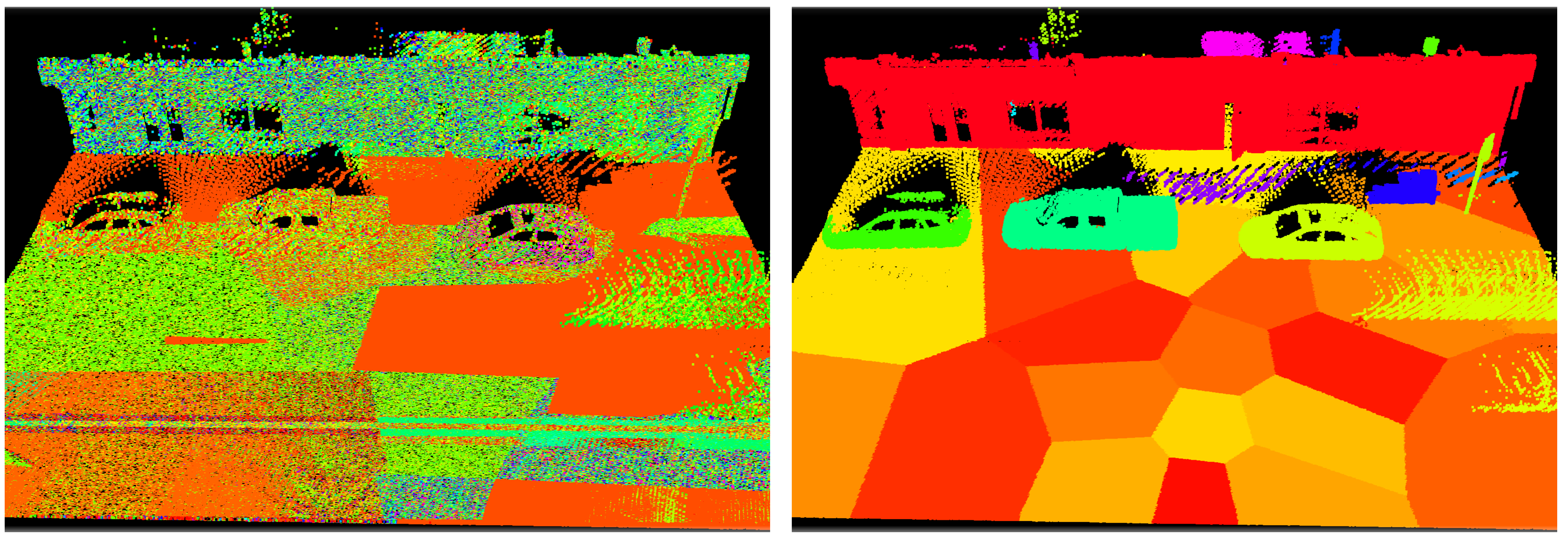
VCCS attempts coherent oversegmentation using local geometry. DBSCAN/HDBSCAN and ground-plane separation are alternatives. These partitions can require substantial preprocessing, and VCCS produces scattered/noisy regions in the authors’ Toronto example. This is an observed failure in their setup, not proof that every supervoxel method fails outdoors.
III-B Region Selection
Compare random regions, heuristic information/diversity scores, and two ensemble scores: variation ratio and predictive entropy. Each point score is averaged within a region before selecting high-scoring regions.
III-B 1 Random
Random region selection is a necessary baseline. Its performance depends on the candidate regions and seed, and it should not be equated with randomly labeling individual scattered points.
III-B 2 Heuristics-based Approaches
ReDAL and SSDR-AL use geometric or feature-space heuristics to supplement network uncertainty. Deep ensembles can improve predictive calibration by averaging independently initialized networks, motivating a simpler ranking rule. This study does not show that ensemble confidence is perfectly calibrated on every dataset.
III-B 3 Variation ratio (VaR)
Train N independently initialized models on the same labels. At each point, variation ratio is one minus the fraction voting for the most common class; average this over the region. Agreement gives zero, even if every model is confidently wrong. Unlike entropy, this score uses class votes rather than the full probability vectors.
Equations 1
| (1) |
III-B 4 Ensemble entropy (Ent)
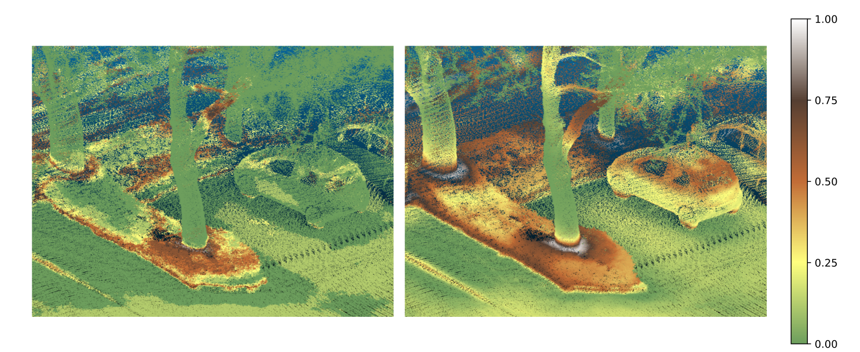
Average the N class-probability vectors, compute the entropy of that average, then average point entropies within a region. This is predictive entropy of the ensemble mean, not mean individual-model entropy or an explicit mutual-information score. Figure 3 shows four-seed SPVCNN uncertainty on Freiburg: both scores highlight vegetation boundaries, but entropy also responds strongly on the car. The displayed normalization is for visualization.
Equations 2–3
| (2) |
| (3) |
III-C Measuring Annotation Effort
A small number of scattered points may span many objects and views, so point count can understate annotation effort. The proposed proxy sums A = ΔxΔy + ΔxΔz + ΔyΔz for each selected region: half the surface area of its axis-aligned bounding cuboid. It measures spatial extent, not true object surface area or observed labor; overlaps and floor-to-ceiling columns can inflate it.
For Toronto, an alternative first removes the ground plane, clusters other points with HDBSCAN, and subdivides the ground using k-means. Figure 4 contrasts these coherent regions with the authors’ noisy VCCS output. The metric is a hypothesis about human workload, without a controlled timing study validating its relationship to actual labeling effort.
IV Experiments
Experiments separately compare area cost, region partitioning, query policies, preprocessing and augmentation. All original plots, numerical tables and uncertainty formulas remain available below.
IV-A Metrics
Mean intersection-over-union measures segmentation quality. “mIoU@90” denotes reaching 90% of the fully supervised model’s mIoU, not 90% absolute mIoU. Query cost is reported either as labeled-point fraction or the summed bounding-cuboid area proxy.
IV-B Datasets
S3DIS has 271 rooms, six areas and 13 classes; evaluation uses Area 5. Toronto-3D covers about one kilometer of road with nine listed classes. Both use color and XYZ inputs.
The private Freiburg cloud spans about 78 km² and 58 billion points. The authors label roughly 42,500 m² across 13 environment-oriented classes, requiring about 85 work hours plus quality assurance. Table I reports approximately 0.15% of points semantically labeled; this is different from the fraction of geographic area annotated. All later Freiburg labeled-data percentages refer to that small labeled subset, not the whole city. Private data and sparse coverage limit reproducibility and generalization claims.
IV-C Network Architecture, Hyperparameters and Codebase
Extend ReDAL’s codebase with SPVCNN and Minkunet backbones. Use Adam at learning rate 0.001, batch size four per GPU, and four ensemble members where applicable; each model trains on one RTX A6000. Ensemble training is extra compute, so preprocessing savings should not be read as equivalent end-to-end speedups.
IV-D Results
Interpret the curves with the same backbone, partition and cost definition where possible. Cross-paper results also differ in code, initialization and sometimes architecture.
IV-D 1 Performance with respect to covered area
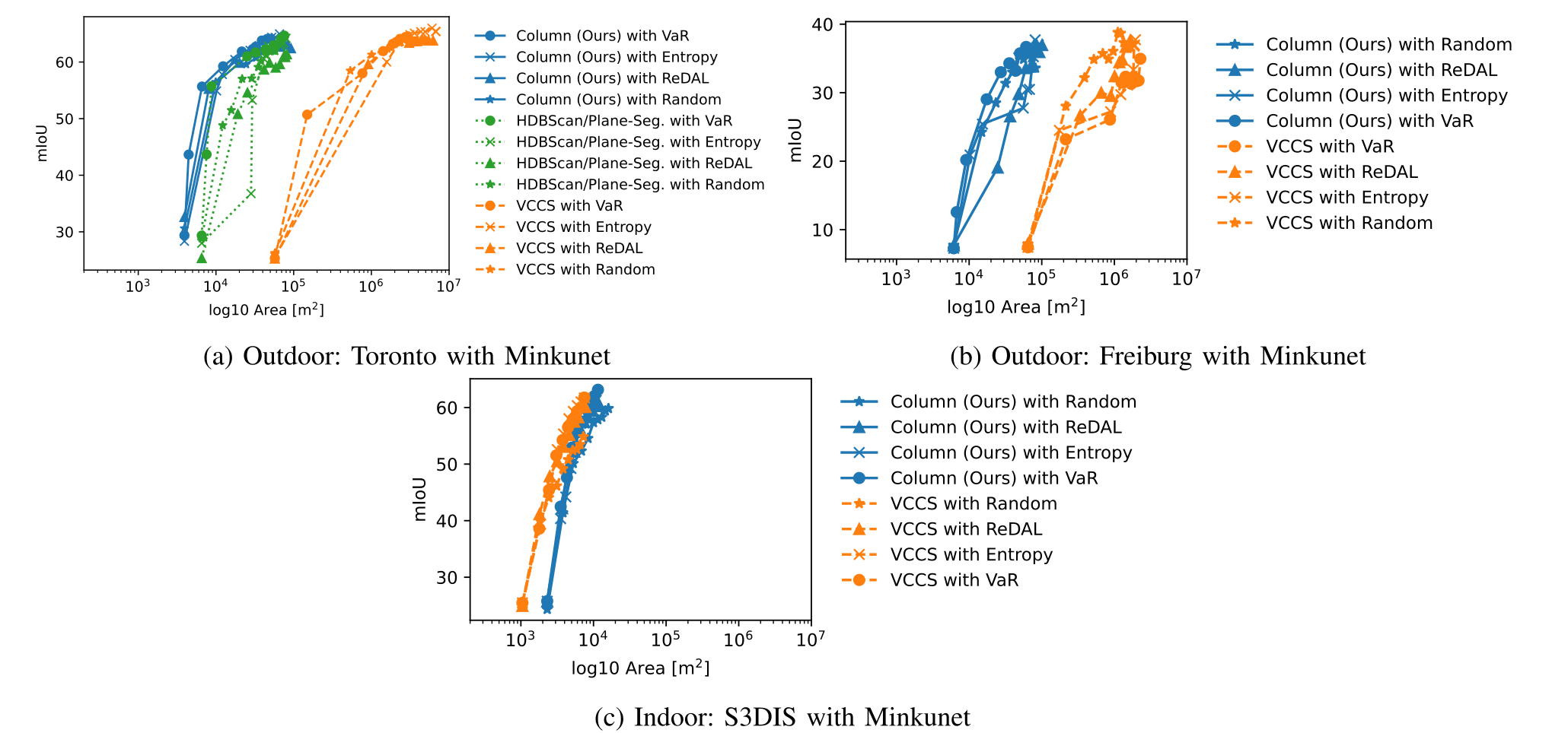
At similar outdoor mIoU, columns use over an order of magnitude less proxy area than VCCS and roughly half that of the HDBSCAN alternative. Indoor S3DIS is closer, with VCCS slightly better: columns include both floor and ceiling, increasing their cuboid area. These are reductions in the proposed proxy, not measured factors of annotation-time reduction.
IV-D 2 Region separation
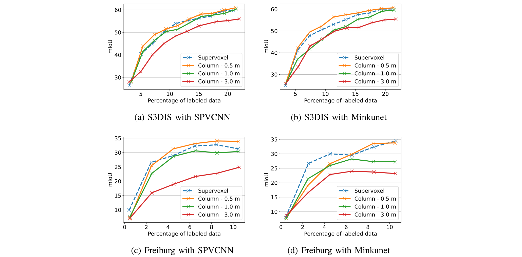
Hold ReDAL selection fixed while changing the partition. Columns of 0.5 m are competitive with supervoxels; 3 m columns perform worse, showing that granularity matters. Freiburg varies substantially across the two backbones, so the authors treat it as supplementary validation rather than the main basis for ranking methods.
IV-D 3 Region selection
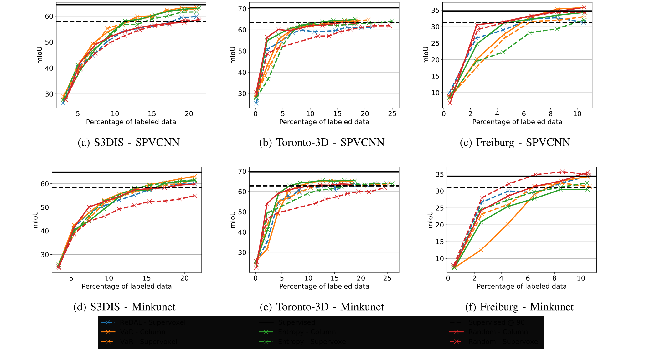
On S3DIS with SPVCNN, Table II gives 11.4% labeled points for column entropy, 13.0% for variation ratio and 21.4% for random columns to reach mIoU@90. The prose says 11.3% for entropy; this minor discrepancy is left explicit. For Minkunet, variation ratio needs 15.4%, better than entropy’s 17.4%. SSDR-AL’s reported 11.7% uses RandLA-Net, so that comparison does not isolate the query policy.
ReDAL reproduced here needs roughly 19%, versus the original report’s 13–15%. On Toronto/SPVCNN, column entropy and variation ratio reach the threshold around 12%/14%, versus 16%/25% for supervoxels. Five-seed Toronto estimates give mIoU standard deviations around 1.4 points early and 0.5 near saturation, moving the crossing by up to about three percentage points of labeled data.
Freiburg is a counterexample to universal superiority: random regions outperform informed policies, and some small-budget models exceed the fully supervised subset baseline. The authors attribute this to noisy/sparse labels, but that explanation is not isolated experimentally. Strong random-region performance also warns against comparisons to weak random-point baselines. The source’s seed-selection discussion cites reference 10, although the relevant Samet study is reference 4.
| Points | |||
| In | Methods | SPVCNN [25] | Minkunet [24] |
| Our | Columns + Random | 21.4 % | 19.4 % |
| Columns + Entropy | 11.4 % | 17.4 % | |
| Columns + VaR | 13.0 % | 15.4 % | |
| ReDAL [7] | 19.0 % | 19.3 % | |
| [7] | ReDAL [7] | 13 % | 15 % |
| [9] | Random [9] | 40.9 % | |
| Entropy [26] | 46.7 % | ||
| BvSB [26] | 43.0 % | ||
| ClassBal [27] | 13.3 % | ||
| SSDR-AL [9] | 11.7 % | ||
IV-E Ablation
The ablations examine preprocessing and augmentation separately from annotation savings. Their measurements should not be combined into a single total-cost claim.
IV-E 1 Preprocessing time
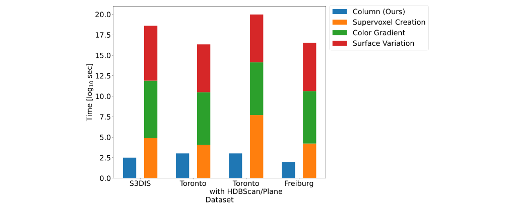
A 50×50 m cloud takes about 0.3 seconds to partition into columns. Reported column preprocessing is 0.59% of the ReDAL-style total on S3DIS, 1.9% on Toronto, 0.64% relative to the Toronto HDBSCAN alternative, and 0.70% on the annotated Freiburg subset. Timing uses a Ryzen 9 Pro 7945 with 64 GB RAM.
Figure 8 stacks quantities labeled log-seconds. Summing log durations is not summing elapsed times, so the graphic should not be used to infer a linear total runtime. The reported ratios concern preprocessing, excluding ensemble training, annotation and inference.
IV-E 2 Data Augmentation
Table III uses randomly sampled 2%/10% files, not actively selected labels. Rotation alone reaches mIoU 27.55/43.23, versus 26.05/41.76 with all augmentations, at lower training-time multipliers. At 100%, all augmentations win with 61.13 versus rotation’s 58.79, but cost 5.92× the no-augmentation baseline. Elastic distortion is especially costly; the chosen active-learning recipe disables it while retaining scale, rotation and chromatic changes.
| 2 % labels | 10 % labels | 100 % labels | ||||||||
|
mIoU |
|
mIoU |
|
mIoU |
| ||||
|---|---|---|---|---|---|---|---|---|---|---|
| 21.67 | 159.00 | |||||||||
| 27.55 | 43.23 | |||||||||
| 61.13 | ||||||||||
V Conclusions
Small columns plus ensemble scores are a practical alternative to elaborate region heuristics, and area accounting reveals a real limitation of point-budget comparisons. The evidence remains dataset- and backbone-dependent: random regions are strong, Freiburg is noisy/private, threshold rankings vary with seeds, and human-time savings are inferred from a proxy. Foundation-model annotation and spatially adaptive grid resolution are proposed future directions.
Acknowledgements
The authors thank the city of Freiburg for its colored LiDAR data and acknowledge German BMU funding through the Intelligence for Cities project.