Overview
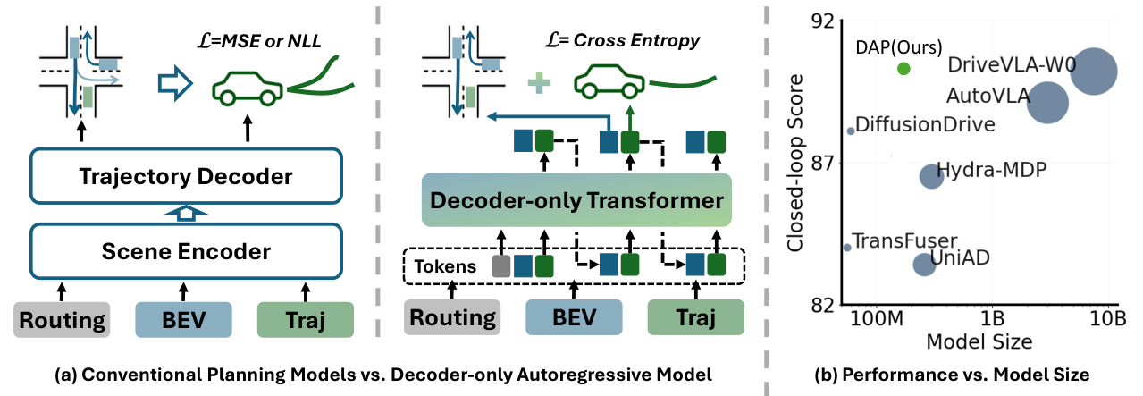
DAP jointly predicts discrete scene and motion tokens for autonomous-driving trajectory planning.
At a glance
DAP is an autoregressive planner that forecasts bird’s-eye-view semantics before selecting ego curvature–acceleration tokens at each future step. Joint supervision supplies scene information beyond sparse trajectory labels, while offline reinforcement learning and trajectory smoothing refine the imitation policy. The reported planner has a 120-million-parameter backbone and scores 90.0 on NAVSIM v1 and 85.6 on v2. These are benchmark results, with remaining comfort and quantization limitations rather than evidence of unrestricted on-road reliability.
1 Introduction
Predicting only expert waypoints gives weak supervision about how the surrounding scene should influence motion. DAP adds a discrete semantic world representation and conditions action generation on its predicted evolution. Autoregression is temporal: scene tokens within a step are generated in parallel, followed by the motion token. The paper combines this architecture with reward-guided fine-tuning and demonstrates gains as training data and token granularity increase; the tested scales do not establish a general scaling law.
2 Related Works
The related work connects autoregressive driving models, compact world forecasting, reinforcement learning, and post-processing of planned trajectories.
2.1 End-to-end Models in Autonomous Driving
Earlier planners use direct trajectory prediction, autoregressive tokens, or explicit scene forecasting. DAP forecasts compact semantic BEV latents instead of rolling out full camera images. This reduces the representation burden while preserving information relevant to lane and obstacle geometry.
2.2 Reinforcement learning for trajectory planning
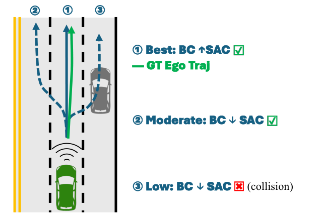
Imitation can assign similar losses to trajectories with different safety margins. DAP adopts an offline variant of SAC-BC [30] to combine reward optimization with a behavior-cloning prior. Related driving systems also combine imitation and reinforcement objectives; the key question here is how that refinement interacts with discrete scene-conditioned planning.
2.3 Trajectory Post-tuning
A rule-based smoothing stage adjusts the learned trajectory using lane geometry and finite-difference penalties. This is part of the evaluated system, so reported comfort cannot be attributed solely to the autoregressive network.
3 Methodology
The pipeline consists of discrete scene/motion modeling, offline reward-guided fine-tuning, and nonlearned trajectory post-tuning.
3.1 Model Structure
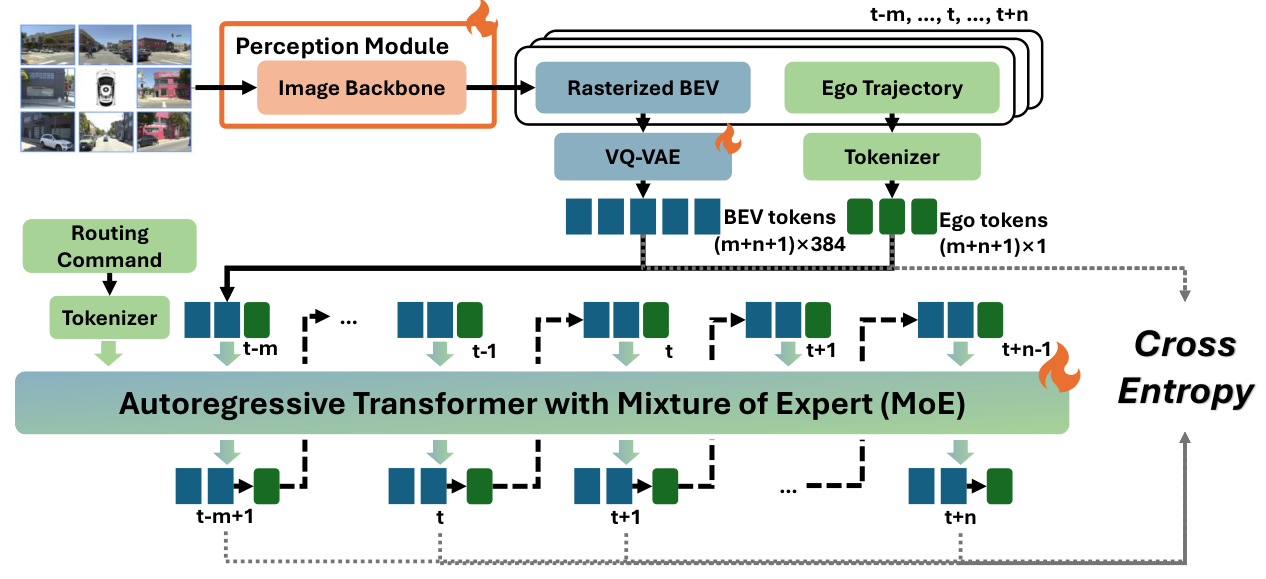
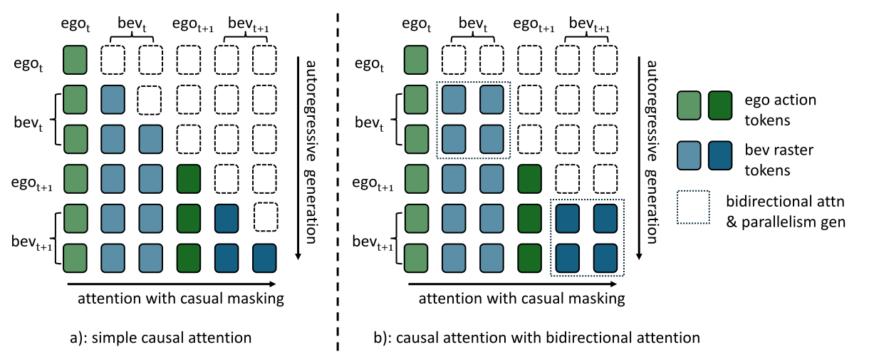
Camera features, ego history, and a high-level command condition a decoder-only mixture-of-experts transformer. Future BEV tokens use bidirectional attention within one time block, while blocks remain temporally causal and the action follows the newly predicted scene. The paper reports about 100 ms for an eight-step trajectory with BEV forecasts, but does not supply enough latency benchmarking detail here to establish full perception-to-control deployment speed.
a) Input Tokenization.
A categorical command is embedded, and a vector-quantized autoencoder [38] maps the semantic BEV grid to codebook indices. Ego poses become finite-difference curvature and acceleration estimates. Curvature bins are finer near zero, acceleration bins are uniform, and the pair can be packed into one action token. The retained equations specify the quantization and conversion, including the low-speed numerical safeguard.
Equations 1–3
| (1) |
| (2a) | ||||
| (2b) | ||||
| (3) |
b) Autoregressive Planning Transformer.
Historical steps concatenate command, scene-token blocks, and action tokens. At each future step, the transformer first emits the entire BEV block in parallel and then emits the action conditioned on that block. A shared vocabulary reserves separate index ranges for modalities. This provides explicit predicted-scene conditioning without fully serial generation of every image-grid token.
Equations 4a–4b
| (4a) | ||||
| (4b) | ||||
c) Training and Inference.
Training minimizes separate cross-entropy losses for scene and action tokens, with a higher weight on motion. Scheduled sampling gradually replaces teacher-forced prefixes with generated tokens to reduce train–test mismatch. The objective encourages useful scene prediction but does not independently prove that every forecasted object motion causally improves the chosen action.
Equations 5–6b
| (5) |
| (6a) | ||||
| (6b) | ||||
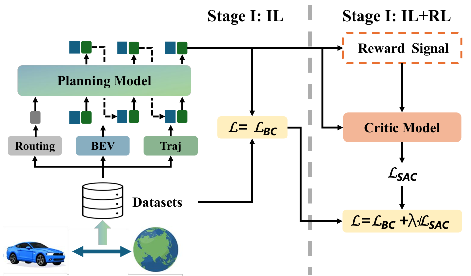
3.2 Reinforcement Learning(RL)
Only trajectory tokens are reinforcement-learning actions; BEV tokens retain supervised training and enter the policy context. Rewards encourage lane-center proximity and obstacle clearance, with acceleration-change and angular-acceleration penalties for comfort. Their geometry is measured in the BEV frame, so usefulness depends on the scene representation and reward design.
Two critics use a soft Bellman target and a conservative penalty on unsupported actions. The discrete actor optimizes the critic-induced objective, while advantage-weighted cloning upweights expert actions valued above the policy baseline. The final loss combines SAC and cloning terms. The complete equations preserve reward masks, entropy and conservative terms, and the value-aware imitation weighting. The illustrative left/right example explains the intended mechanism rather than constituting a safety guarantee.
Equations 7–12
|
|
(7) |
| (8) |
| (9) |
| (10) |
| (11) | ||||
| (12) |
3.3 Trajectory Post-tuning
Discrete tokens can create small lateral oscillations or abrupt motion changes. The post-tuning stage finds lane anchors from a likelihood map and solves a regularized least-squares problem in a local Frenet frame. First- and second-difference penalties smooth lateral and longitudinal motion, after which yaw is recomputed and rate-limited. The displayed objective improves geometric alignment and comfort but is not a formal collision-avoidance certificate.
Equations 13–14
| (13) |
| (14) |
4 Experiments
Experiments separate open-loop trajectory error from simulation-derived planning scores, then ablate supervision, fine-tuning, data scale, and token resolution.
4.1 Implementation Details
NAVSIM training uses 2 Hz data, four initial cloning epochs, and a sixteen-epoch total schedule with AdamW on four A800 80 GB GPUs. A pretrained roughly 50-million-parameter TransFuser encoder is further fine-tuned to supply BEV features. The paper separately describes a 120-million-parameter planner backbone; it does not clearly reconcile these components into a complete system parameter count. The nuScenes model is separately trained with cloning only.
| Model | (m) | (m) | ||||||
|---|---|---|---|---|---|---|---|---|
| 1s | 2s | 3s | Avg. | 1s | 2s | 3s | Avg. | |
| VAD [18] | 0.41 | 0.70 | 1.05 | 0.72 | – | – | – | – |
| BridgeAD [46] | 0.28 | 0.55 | 0.92 | 0.58 | – | – | – | – |
| UniAD [14] | 0.42 | 0.64 | 0.91 | 0.66 | 0.48 | 0.96 | 1.65 | 1.03 |
| SparseDrive [37] | 0.29 | 0.58 | 0.96 | 0.61 | – | – | – | – |
| SSR [22] | 0.19 | 0.36 | 0.62 | 0.39 | 0.25 | 0.64 | 1.33 | 0.74 |
| OpenDriveVLA [48] | 0.15 | 0.31 | 0.55 | 0.33 | 0.20 | 0.58 | 1.21 | 0.66 |
| EMMA∗ [17] | 0.14 | 0.29 | 0.54 | 0.32 | – | – | – | – |
| EMMA+∗ [17] | 0.13 | 0.27 | 0.48 | 0.29 | – | – | – | – |
| MAX-V1∗ [44] | 0.24 | 0.38 | 0.65 | 0.42 | 0.28 | 0.63 | 1.41 | 0.77 |
| Ours (DAP) | 0.12 | 0.27 | 0.44 | 0.27 | 0.21 | 0.50 | 1.00 | 0.57 |
| Method | Val4k Set | Test4k Set | Val14 Set | ||||||
|---|---|---|---|---|---|---|---|---|---|
| 8sADE | 8sFDE | OLS | 8sADE | 8sFDE | OLS | 8sADE | 8sFDE | OLS | |
| PlanCNN [31] | – | – | – | – | – | – | 2.468 | 5.936 | 64 |
| PDM-Hybrid [10] | 2.435 | 5.202 | 84.06 | 2.618 | 5.546 | 82.04 | 2.381 | 5.068 | 84 |
| PlanTF [7] | 1.774 | 3.892 | 88.59 | 1.855 | 4.042 | 87.30 | 1.697 | 3.714 | 89.18 |
| DTPP [16] | 4.196 | 9.231 | 65.15 | 4.117 | 9.181 | 64.18 | 4.088 | 8.846 | 67.33 |
| STR2-CKS-800m [36] | 1.473 | 4.124 | 90.07 | 1.537 | 4.269 | 89.12 | 1.496 | 4.219 | 89.2 |
| Ours (DAP) | 1.202 | 3.711 | 91.68 | 1.393 | 4.090 | 90.16 | 1.311 | 3.942 | 91.02 |
- •
Note: Bold indicates the best result.
4.2 Open-loop Evaluation
On nuScenes, the table reports average L2 trajectory error 0.27 m and average L2max 0.57 m, the best aggregate values among listed entries. At one second, OpenDriveVLA has slightly better L2max, 0.20 versus 0.21 m. On nuPlan, DAP has the best listed eight-second average displacement and open-loop score across all three splits, including 1.202 m and 91.68% on Val4k. PlanTF has lower final displacement error on Test4k and Val14. These are prediction/trajectory metrics rather than collision-free execution results.
| Method | Ref | Sensors | NC | DAC | TTC | C. | EP | PDMS |
|---|---|---|---|---|---|---|---|---|
| Human | – | – | 100 | 100 | 100 | 99.9 | 87.5 | 94.8 |
| UniAD [14] | CVPR’23 | C | 97.8 | 91.9 | 92.9 | 100.0 | 78.8 | 83.4 |
| TransFuser [9] | TPAMI’23 | C + L | 97.7 | 92.8 | 92.8 | 100.0 | 79.2 | 84.0 |
| DiffusionDrive [29] | CVPR’25 | C + L | 98.2 | 96.2 | 94.7 | 100.0 | 82.2 | 88.1 |
| WoTE [26] | ICCV’25 | C + L | 98.5 | 96.8 | 94.4 | 99.9 | 81.9 | 88.3 |
| MeanFuser [40] | CVPR’26 | C | 98.6 | 97.0 | 95.0 | 100 | 82.8 | 89.0 |
| AutoVLA [49] | NeurIPS’25 | C | 98.4 | 95.6 | 98.0 | 99.9 | 81.9 | 89.1 |
| ReCogDrive [27] | arXiv’25 | C | 98.2 | 97.8 | 95.2 | 99.8 | 83.5 | 89.6 |
| DriveVLA-W0∗ [25] | ICLR’26 | C | 98.7 | 99.1 | 95.3 | 99.3 | 83.3 | 90.2 |
| Ours (DAP) | – | C | 98.1 | 97.9 | 97.7 | 100.0 | 86.8 | 90.0 |
- •
Note: Bold indicates the best result. ∗ indicates the best variant of DriveVLA.
| Method | NC | DAC | DDC | TLC | EP | TTC | LK | HC | EC | EPDMS |
|---|---|---|---|---|---|---|---|---|---|---|
| Ego Status | 93.1 | 77.9 | 92.7 | 99.6 | 86.0 | 91.5 | 89.4 | 98.3 | 85.4 | 64.0 |
| TransFuser [9] | 96.9 | 89.9 | 97.8 | 99.7 | 87.1 | 95.4 | 92.7 | 98.3 | 87.2 | 76.7 |
| HydraMDP++ [28] | 97.2 | 97.5 | 99.4 | 99.6 | 83.1 | 96.5 | 94.4 | 98.2 | 70.9 | 81.4 |
| DriveSuprem [45] | 97.5 | 96.5 | 99.4 | 99.6 | 88.4 | 96.6 | 95.5 | 98.3 | 77.0 | 83.1 |
| DiffusionDrive [29] | 98.2 | 95.9 | 99.4 | 99.8 | 87.5 | 97.3 | 96.8 | 98.3 | 87.7 | 84.5 |
| DriveVLA-W0 [25] | 98.5 | 99.1 | 98.0 | 99.7 | 86.4 | 98.1 | 93.2 | 97.9 | 58.9 | 86.1 |
| MeanFuser [40] | 98.3 | 97.2 | 99.6 | 99.8 | 87.6 | 97.4 | 97.3 | 98.3 | 88.2 | 89.5 |
| Ours (DAP) | 97.1 | 95.2 | 98.8 | 99.7 | 88.4 | 95.7 | 95.9 | 98.9 | 70.3 | 85.6 |
- •
Note: Bold indicates the best result.
4.3 Closed-loop Evaluation on NavSim v1
On NAVSIM v1 [11], DAP scores 90.0 PDMS, versus 90.2 for the listed DriveVLA-W0 variant and 94.8 for the human reference. Its progress score is 86.8, comfort score 100.0, time-to-collision score 97.7, and drivable-area compliance 97.9. The table mixes camera-only and camera-plus-LiDAR systems, with DAP marked camera-only. The favorable size/score comparison therefore spans different architectures, data, and inputs.
4.4 Closed-loop Evaluation on NavSim v2
The NAVSIM v2 protocol [4] adds direction, traffic-light, lane-keeping, and further comfort terms. DAP reaches 85.6 EPDMS, below MeanFuser’s 89.5 and DriveVLA-W0’s 86.1. Progress 88.4 ties DriveSuprem, while history comfort 98.9 leads this table. Extended comfort is only 70.3, identifying a substantive weakness obscured by the perfect v1 comfort subscore. These data-driven benchmark scores do not replace a reactive traffic or physical-road deployment evaluation.
4.5 Qualitative Results
Figure 6 preserves the full side-by-side motion and semantic forecasting examples. Each scenario contains a current-view trajectory plus three future BEV predictions, alongside matching ground truth. The examples illustrate aligned scene and motion forecasts; no separate quantitative world-prediction accuracy study is reported here.

4.6 Ablation Study
At the reported 20,000-example objective setting, trajectory-only planning scores 82.8, joint scene/action cloning 84.6, and SAC-BC 85.4. In the separately listed tokenization sweep, finer 16-fold downsampling with a 512-entry codebook improves from 85.8 to 87.7 to 88.7 as data grows from 20,000 to 50,000 to 80,000 examples. Enlarging that codebook to 1,024 reaches 90.0; the coarser 32-fold grid reaches only 86.6. These ablations support the tested combination, while the table does not explain the differing 20,000-example scores between its two groups.
5 Conclusion
Joint discrete scene forecasting, action prediction, offline fine-tuning, and smoothing produce a compact competitive planner in the reported benchmarks. Important limits are token-induced motion jitter, lower extended comfort, dependence on the perception representation and reward design, and the absence of a demonstrated broad scaling law or physical driving evaluation. The paper has no separate appendix or limitations section; the original media, equations, and references are retained.