Intuition. Making two views produce the same vector is easy if every image produces zero. LeJEPA adds a second requirement: across different examples, embeddings should form a well-spread, approximately Gaussian cloud. Agreement encourages shared information; distribution regularization prevents an uninformative constant solution.
SIGReg checks many one-dimensional projections of that cloud, avoiding a full high-dimensional density estimate. The paper combines this construction with theory about downstream probes and experiments across architectures and domains. Its guarantees depend on the specified statistical assumptions; a Gaussian embedding alone does not identify the semantic features or prove a useful physical world model.
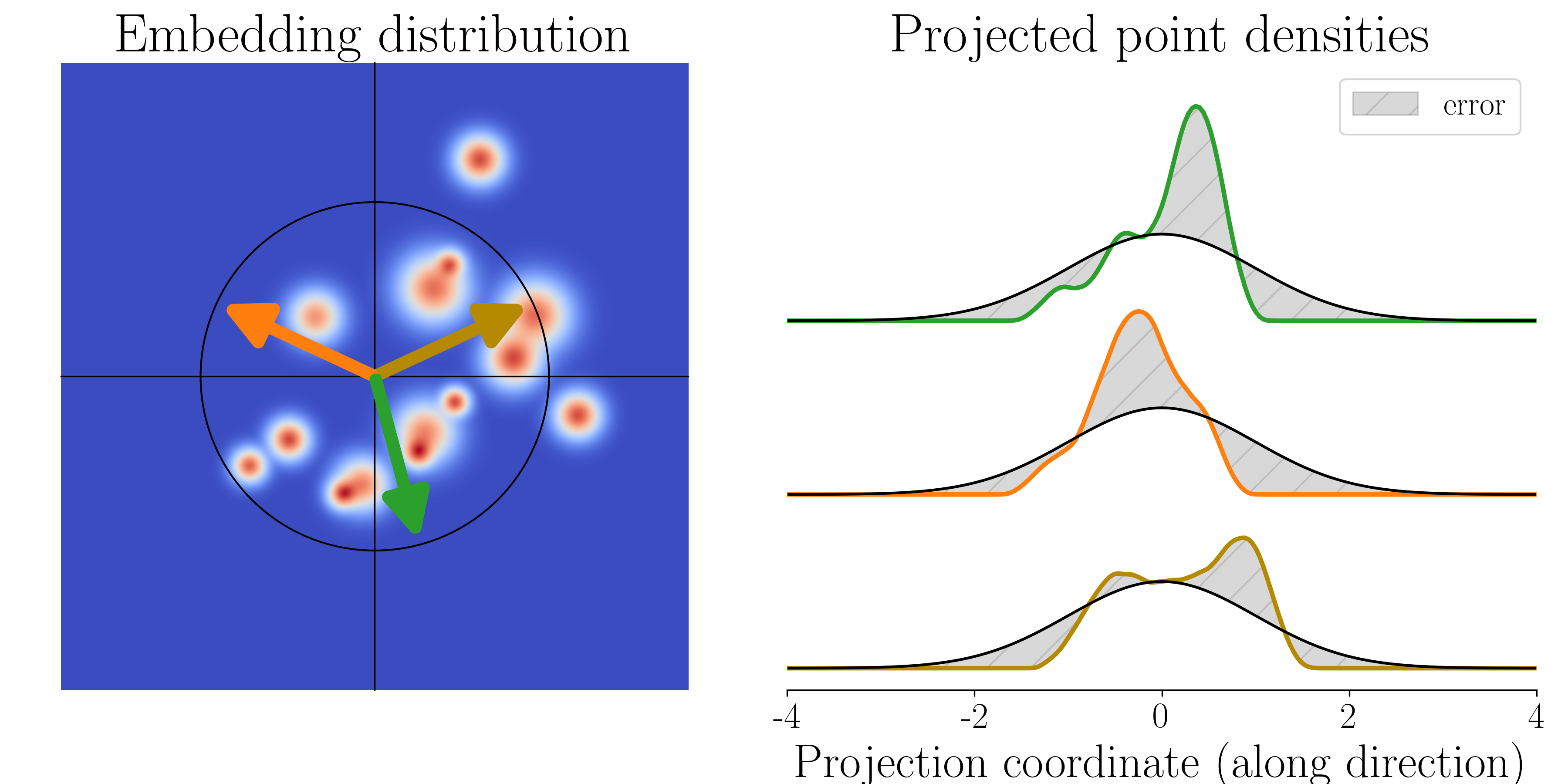
Figure 2: Sketched Isotropic Gaussian Regularization (SIGReg): Given some arbitrary input data with density with support that may or may not lie on a manifold (left), a Deep network (DN) encoder () produces embeddings with some distribution (middle). Our proposed Backward Cramér-Wold Statistics (Section4) objective pushes to match a target distribution by projecting the embeddings along directions (middle, arrows) and enforcing that the univariate densities (right, colored lines) match the distribution of , projected along the same directions. Any popular statistical test (provided in Section4.2) can assess the goodness-of-fit–in practice we argue for characteristic function tests (Section4.2). By using SIGReg with isotropic Gaussian (right, black lines), we introduce a lean and provably optimal (Section3) JEPA, coined LeJEPA, free of numerous heuristics and able to produce competitive performances (Sections5 and 6).
1 Introduction
The method separates two design decisions: choose related views whose shared content should be retained, and prevent the representation from collapsing while those views are aligned. LeJEPA supplies an explicit regularizer for the second decision. It removes several teacher–student training mechanisms in the tested recipe, while retaining ordinary choices such as architecture, augmentations, optimizer and training budget.
2 Background and Notations
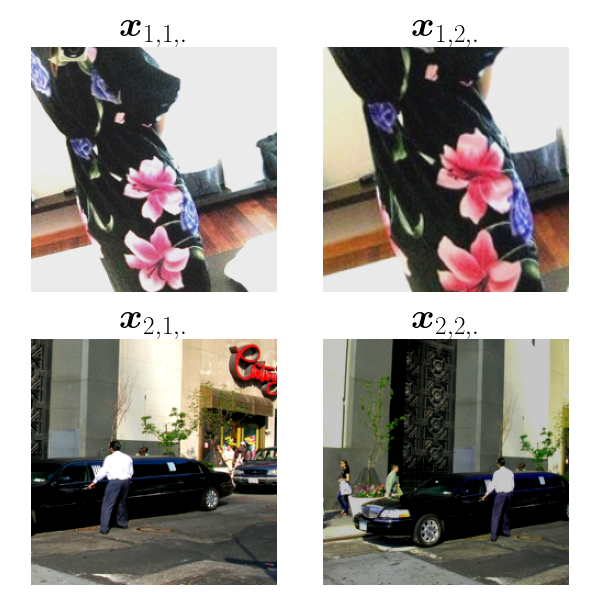
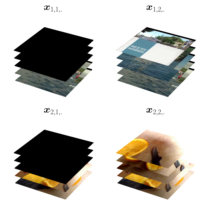
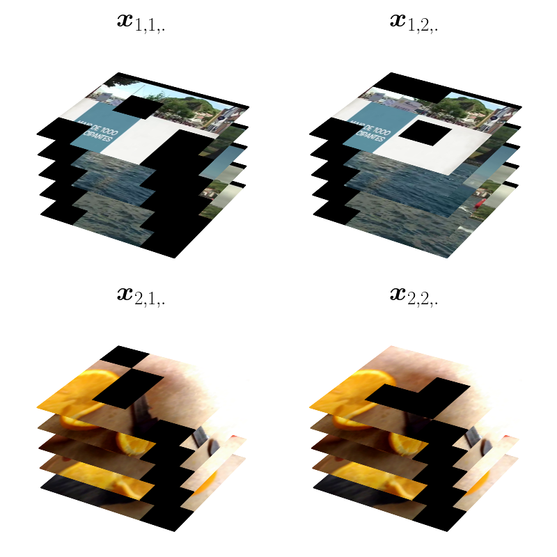
The notation distinguishes independent training examples, related views of each example and the coordinates of an embedding. This separation is essential: similarity within a view group and diversity across examples play different roles.
2.1 Notations and Definitions
Inputs are organized as examples × views × input coordinates. A neural network maps each view to an embedding. Independence assumptions concern different examples, not necessarily views of the same example. The downstream probe is a separately trained prediction rule, so a statement about its statistical risk is not automatically a statement about arbitrary end-to-end tasks.
A low agreement loss does not rule out shortcut representations. Whitening, contrastive negatives and asymmetric moving-teacher designs address this in different ways. LeJEPA asks for a direct, scalable distribution constraint instead of treating a successful teacher recipe as the only available collapse-prevention mechanism.
2.3 The Need for Actionable Theory
Theory is used to motivate an implementable objective rather than only explain a completed training run. The paper studies particular probe families and statistical assumptions. Its design principle is most useful when those assumptions and the chosen views are kept visible alongside the empirical results.
3 Latent Euclidean: Embeddings Should be Isotropic Gaussian
The theoretical target is an isotropic Gaussian: a centered Gaussian distribution with equal variance in every direction. This is a geometric preference under the paper’s fixed-energy and downstream-risk formulations, not a proof that all useful data must be Gaussian or that arbitrary labels become predictable after Gaussianization.
3.1 Linear Probing
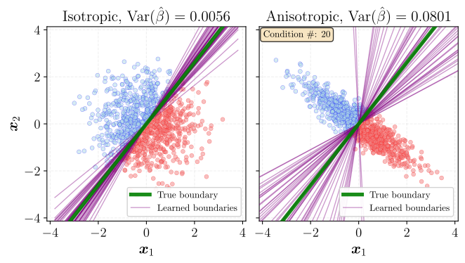
For linear probes, compare embeddings spanning the same features and having the same total variance, but distributing that variance differently across directions. Uneven covariance can amplify estimation variance and regularization bias for unfavorable downstream target directions. Isotropy improves these worst-case geometric properties. This comparison controls the available features; it does not show that replacing informative features with arbitrary Gaussian noise is beneficial.
Whenever , there always exists a downstream task () for which produces a higher bias estimator than for . (Proof in SectionB.1.)
Lemma 2: Anisotropy amplifies variance
With , the total variance of (OLS) is minimized for with
. (Proof in SectionB.2.)
3.2 Nonlinear Probing
The nonlinear analysis considers radius-based neighbors and kernel regression, with smooth densities, smooth target functions and specified variance or geometric constraints. Under the paper’s risk formulation, a Gaussian shape emerges as optimal. These regularity and target-class assumptions are part of the claim; they cannot be dropped when applying the conclusion to a new task.
and among distributions with a scalar-based covariance constraint, the isotropic Gaussian is the unique minimizer of the integrated square bias. (Proof in SectionsB.4 and B.7.)
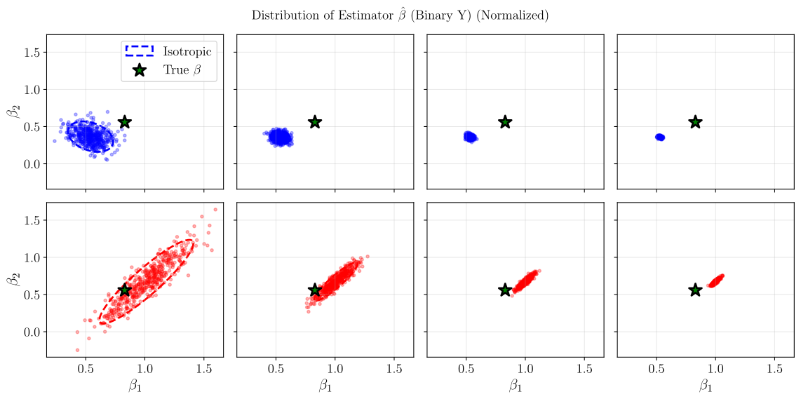
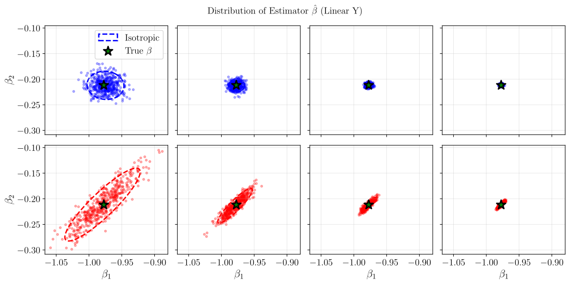
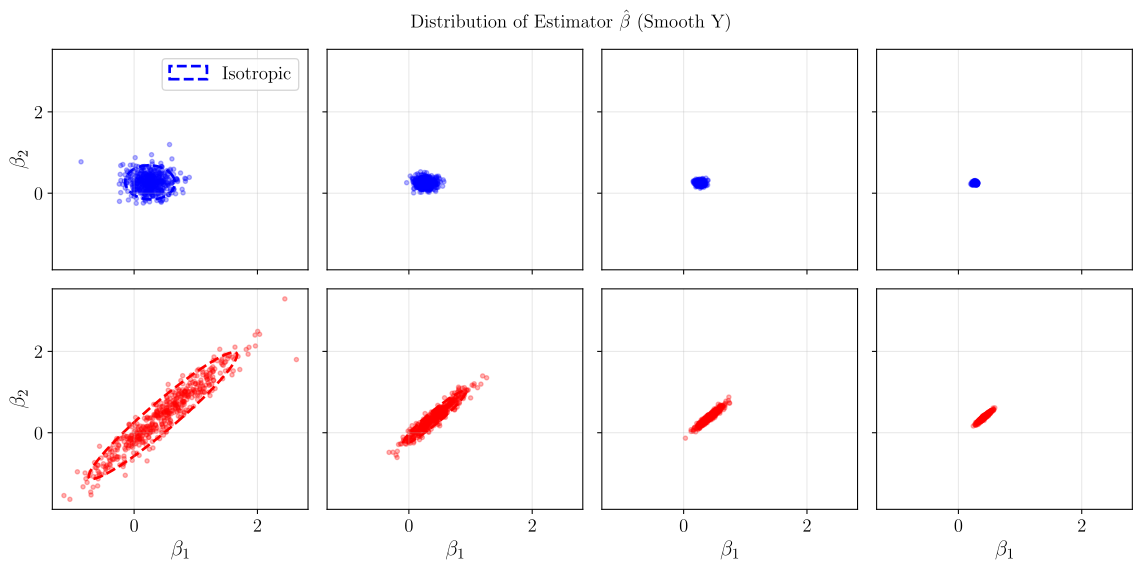
Figure 3: Illustration of Section3.1 showcasing how anisotropic (right) embeddings lead to higher variance estimator compared to isotropic embeddings (left). We sample training points for the -class classification task and fit a logistic regression–repeating the process over numerous training set sample. Each sampling results in a decision boundary (purple).
3.3 Geometric and Practical Insights
Synthetic examples illustrate why poorly scaled directions make probe fitting less stable. Equalized directions reduce this geometric disadvantage. For a reader, the useful distinction is between making existing information easier to read and learning the right information in the first place.
4 SIGReg: Reliable Isotropic Gaussian Regularization in High-Dimension
SIGReg turns the Gaussian target into a differentiable training penalty. It compares projected embedding samples with the desired one-dimensional Gaussian and aggregates across projection directions.
4.1 Hypothesis Testing as a Judge
A distribution test asks whether observed samples provide evidence against the Gaussian target. Failure to reject is not proof of equality. At the population level, matching every one-dimensional projection identifies the full distribution; finite samples and finitely many directions need additional coverage and regularity arguments.
Equations 2–4
(2)
(3)
(4)
Lemma 3: Hyperspherical Cramér-Wold
Let be -valued random vectors, then
Equation
Convergence in distribution also holds. (Proof in SectionB.8.)
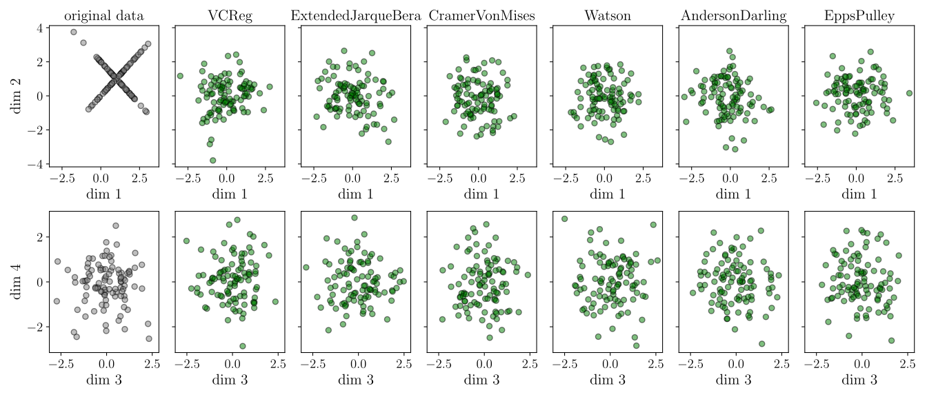
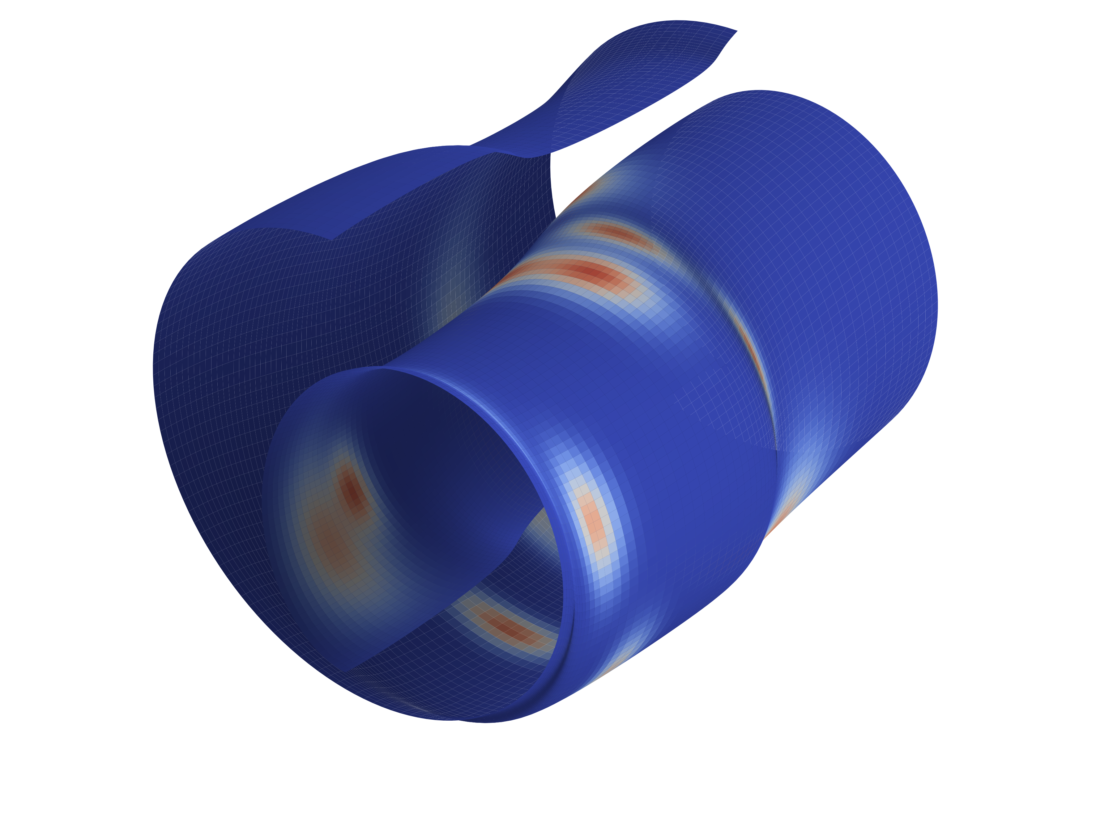
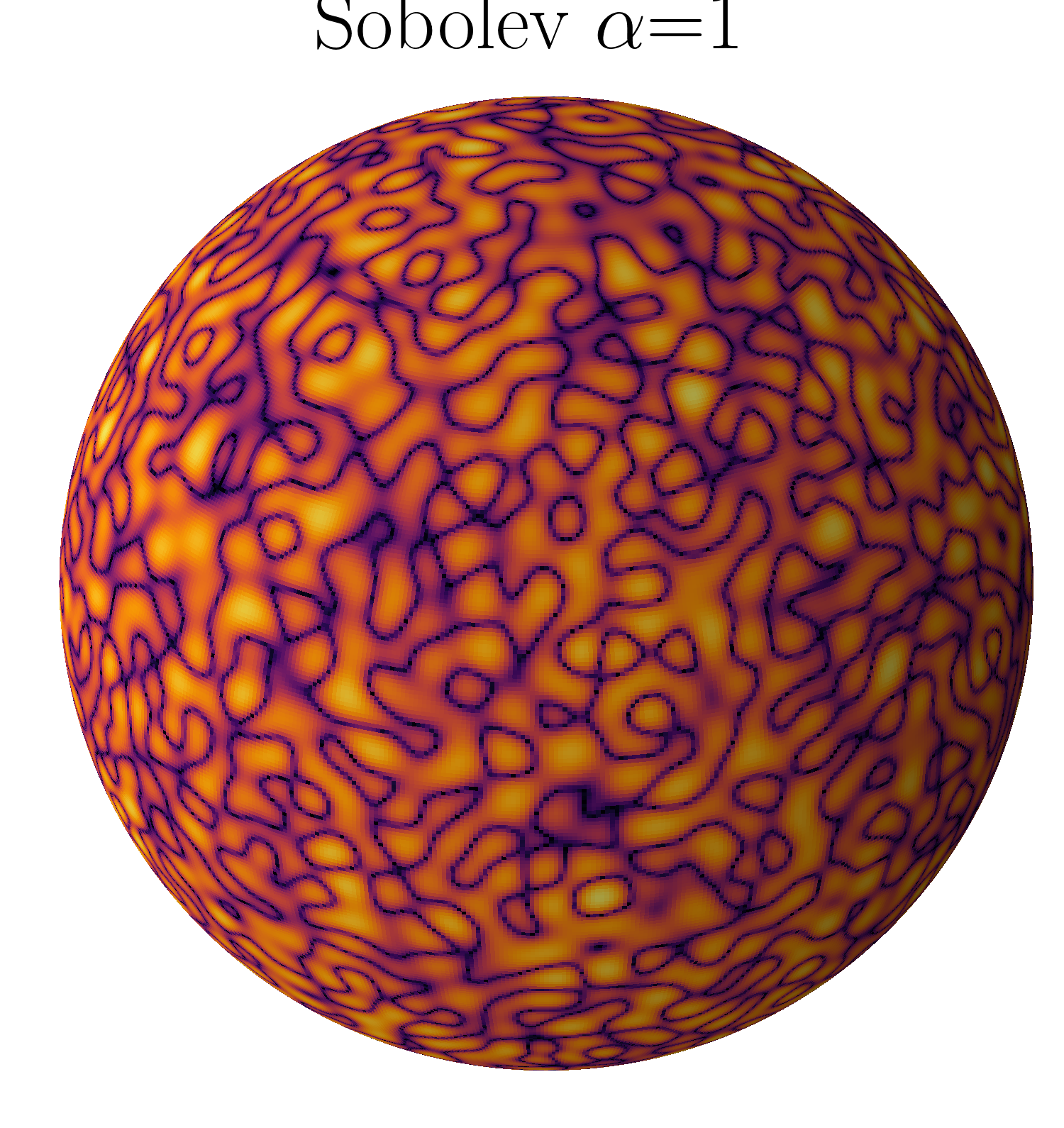
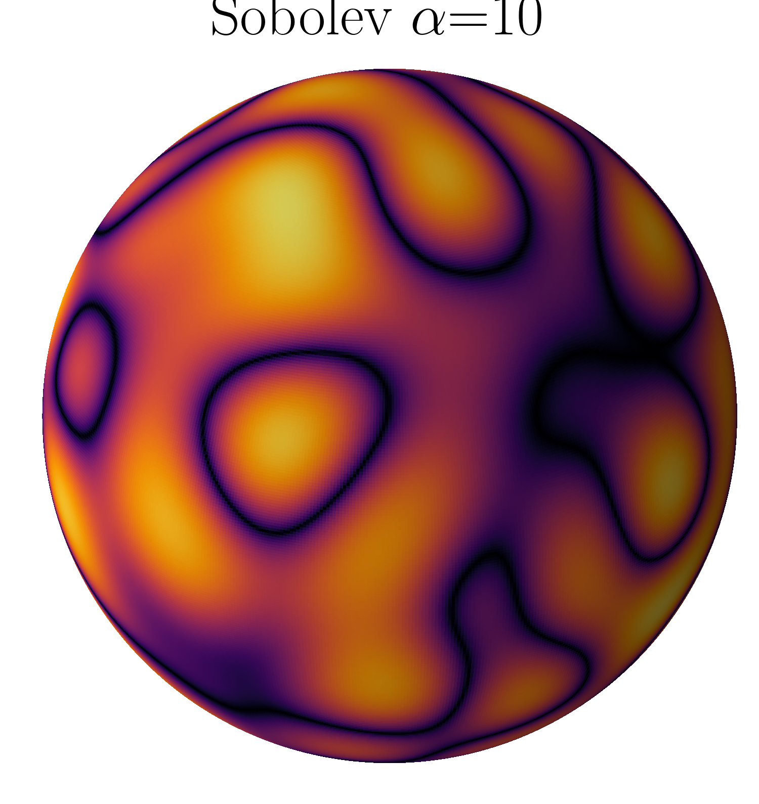
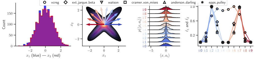
Figure 4: Examples of distributions living on the surface of the sphere with varying Sobolev smoothness coefficients . As per Section4.3, the greater is, the more global will be the impact of SIGReg for a given number of directions . Practically, this represents the distribution of the encoder’s output. Because the target density (isotropic Gaussian) is smooth, the coeffcients of the embedding will quickly grow hereby making SIGReg (Section4.2) immune to the curse of dimensionality.Figure 5: Constructed data density with “X” distribution whose marginals are standard Gaussian and whose covariance is identity (left densities). Applying projections on the half circle directions produces univariate distributions that can be compared against a standard Gaussian (left) using any preferred statistic from Section4.2. The appropriate direction is able to capture the degenerate distribution of the data hereby creating a spike in the statistic value.
4.2 SIGReg: Sketching the Epps-Pulley Test is Stable and Scalable
The method averages projection-wise penalties to supply learning signal across directions. The choice of one-dimensional statistic matters for both what departures it detects and how stable its gradients are.
SIGReg sketches a statistical test towards isotropic Gaussian
Equation(5)
where we recommend the Epps-Pulley test (Section4.2.3) for .
4.2.1 Moments are Unstable and Insufficient
Matching only a finite number of moments leaves different distributions indistinguishable. High powers of large samples can also create unstable gradients. The paper uses these two issues to motivate a statistic that describes more of the distribution without relying on high-order polynomial moments.
Equations Jarque-Bera–Extended Jarque-Bera
(Jarque-Bera)
(Extended Jarque-Bera)
Theorem 3: Insufficiency of K Moments
Minimizing the following objective with
Equation
for finite does not imply . (Proof in SectionB.11.)
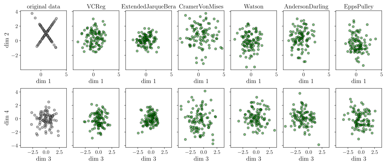
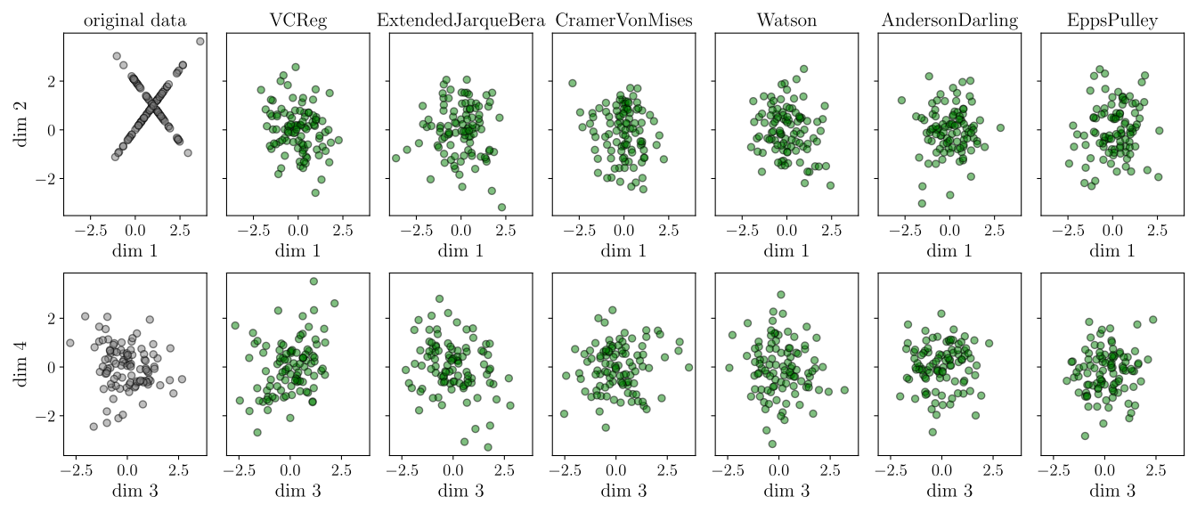
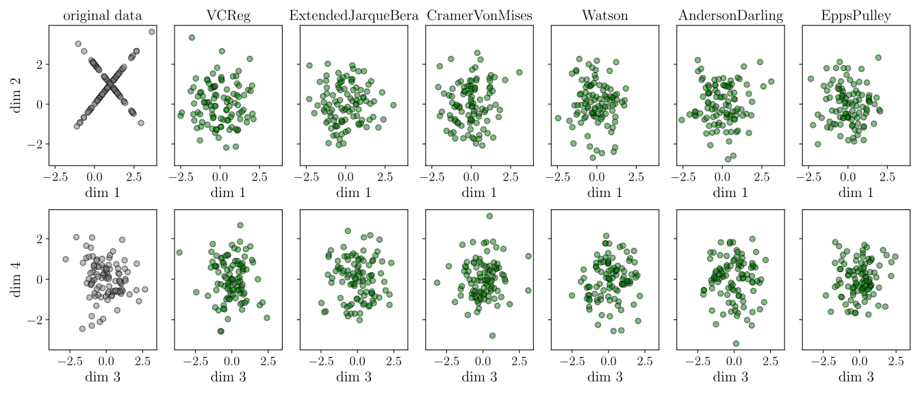
Figure 6: samples are drawn from a -dimensional standard Gaussian, and the first coordinates are altered to produce the “X” distribution from Figure5 (left-most column). For each statistic (all other columns), we perform gradient descent on the samples to minimize their value, at each iteration step with sample random directions to evaluate SIGReg (recall Section4.2). We obtain that albeit this is a high-dimensional distribution with limited number of samples, SIGReg is able to capture the degenerate subspace and adapt the data accordingly to match an isotropic Gaussian distribution. Additional figures with varying dimensions and number of 1d projections are provided in Figure16.
4.2.2 Cumulative Density Functions are Impractical
The discussed cumulative-distribution tests require sorting or related order statistics, which complicate efficient distributed differentiation. This is an implementation motivation for the chosen alternative, rather than a claim that such tests have no statistical value.
Equations Cramér-von Mises–Watson
(Cramér-von Mises)
(Anderson-Darling)
(Watson)
4.2.3 Characteristic Functions are Stable, Scalable and Identifiable
A characteristic function summarizes a distribution through averages of complex exponentials, a Fourier-style description. The Epps–Pulley penalty compares this summary with that of a Gaussian over a weighted frequency range. Its bounded trigonometric components support the stated gradient and curvature bounds, and sample averages can be combined efficiently across devices.
with constant , and bandwidth . (Proof in SectionB.12.)
SIGReg with Epps-Pulley statistic with DDP support and time and memory complexity. x is a (N, K) tensor, num_slices is in Section4.2, ‘global_step‘ is used for sync. sampling across GPUs and can be omited for single-GPU training. An optimized implementation with caching is also provided in our official codebase, computation times provided in Table6.
Finite projection coverage is the practical issue: how many directions are enough to detect a departure from Gaussianity? The following arguments combine smoothness assumptions, resampling during training and controlled experiments.
Smoothness Beats the Curse of Dimensionality
Smoothness can relate a discrepancy on untested directions to discrepancies on tested directions. The rate depends on embedding dimension, smoothness and how directions cover the sphere. The resulting bounds are conditional; a few projections are not an unconditional certificate of an arbitrary high-dimensional distribution.
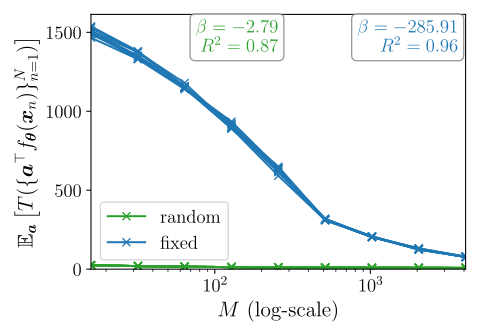
Figure 7: Expected directional statistic at the end of training (y-axis) for varying (number of directions used at each training step, x-axis). The directions are either resampled (green) or kept fixed (blue) at each training step. While for fixed directions we benefit from Section4.3 bound where increasing reduces the overall expected loss, being able to resample at every step provides significant coverage boost for free.
Drawing new directions on successive minibatches covers more possibilities than repeatedly testing one small fixed set. The paper’s experiments compare these choices. The accumulated training signal should still be distinguished from a finite-sample hypothesis-test guarantee at one fixed checkpoint.
Empirical Validation on Synthetic Data
The synthetic experiment inserts a difficult two-dimensional non-Gaussian pattern into an otherwise Gaussian high-dimensional cloud. Optimizing samples directly tests whether projection penalties can find and remove that defect, separately from encoder architecture and semantic learning.
The implemented objective combines view prediction/agreement and SIGReg. A mixing coefficient balances the two. Computational approximations make the distribution penalty practical without constructing all pairwise sample distances.
The characteristic-function integral is approximated with a short deterministic quadrature grid. Minibatch estimation introduces a bias of order inverse batch size in the stated calculation; numerical quadrature adds a separate approximation. Global and local views supply prediction pairs. The core loss can be short, but the complete training system still requires data, augmentation, architecture and optimization settings.
LeJEPA implementation–works out-of-the-box on any dataset, with DDP, with any backbone, e.g., torchvision or timm. For non-ViT architectures (e.g., ResNet), set global_views = all_views. We use bs for the minibatch size, SIGReg is from .
therefore both the loss and its derivative have a bias of order . (Proof in SectionB.13.)
Equations 6–9
(6)
(7)
(8)
(9)
5.2 Relation to Prior Work
Random-projection distribution matching connects to sliced methods and kernel discrepancies. In a limiting moment-matching choice, the framework recovers mean and covariance conditions related to VICReg. The Gaussian-testing version constrains more than those first two moments.
The experiments separately examine training stability, loss-based model selection, domain-specific pretraining, larger backbones and qualitative semantic features. Each supplies evidence for a different part of the proposed recipe.
6.1 LeJEPA’s Stability Across Hyper-Parameters and Architectures
Ablations vary loss weight, number of views, minibatch size, projection count, integration settings and backbone. The paper recommends a practical starting recipe and reports broad stability in those ranges. SIGReg is not literally parameter-free: its numerical settings and the surrounding training choices still exist even when defaults transfer well.
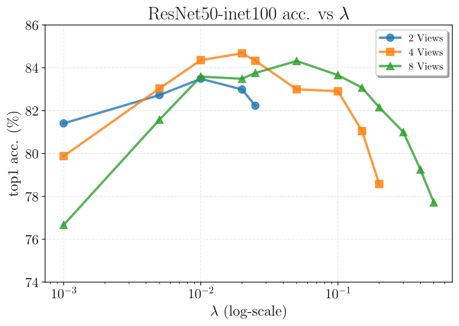
Figure 8: Inet100 with pretraining epochs and resnet50 backbone. We depict linear probe performances as a function of and the number of views (recall (9)). We observe that performances are stable over –with peak performance obtain by slightly adjust proportionally to the number of views. The corresponding performance values are provided in Table7.
Table 1: ViT/Large-14, on inet1k pretraining for 100 epochs and evaluated with frozen backbone linear probing (top1 accuracy, %).LeJEPA’s performance is stable across all its hyperparameters and while some may slightly improve performance, e.g., the number of slices and the projector sizes, none of the choices lead to a catastrophic collapse.
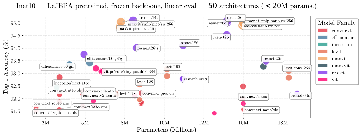
Figure 9: INet10 pretraining and frozen backbone linear evaluation across timm models using LeJEPA out of the box. We cross-validate the learning rate and weight-decay. While there is a small variation between the best and worst performing model, we clearly see that across models spanning families, LeJEPA is able to produce non-trivial representations able to solve the downstream task at SOTA levels.
Experiment Details 1
We strive for simplicity and thus adopt a unified pretraining pipeline. The following parameters apply to all experiments and figures unless stated otherwise in the corresponding caption and come from Section6.1:
•
LeJEPA’s implementation is given in with hyperparameter
•
All backbones are from and all optimizers/schedulers are from without modifications
•
We employ eight views () containing two global views () with resolution 224x224 and 96x96 for the local views
•
AdamW optimizer with and –no scheduler on weight-decay, standard linear warm-up cosine-annealing for
6.2 LeJEPA’s Training Loss is Informative of Downstream Performance
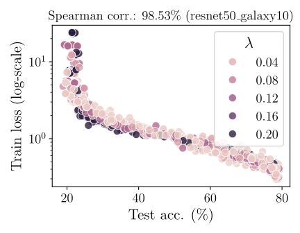
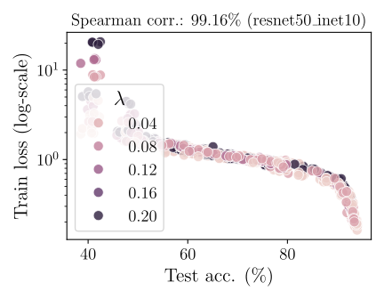
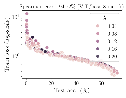
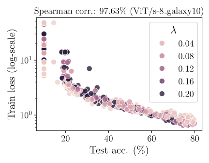
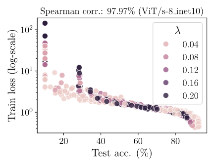
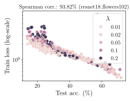
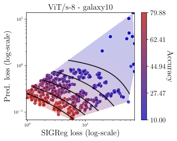
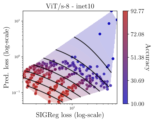
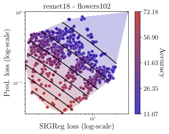
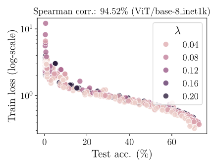
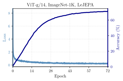
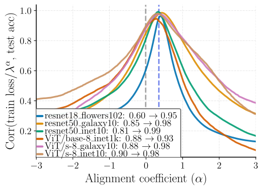
Across the tested runs, lower combined training loss correlates strongly with higher downstream accuracy. This makes it a potentially useful monitoring signal. Correlation in these experiments is not a guaranteed quality ordering for every future dataset, label set or checkpoint.
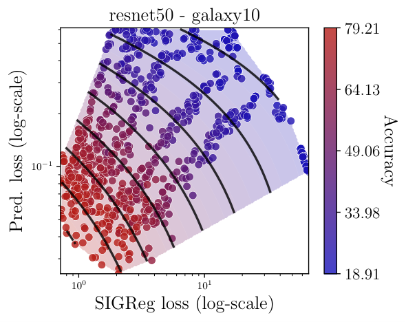
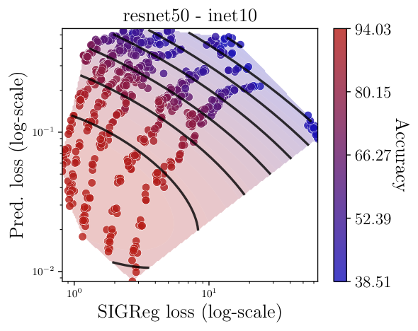
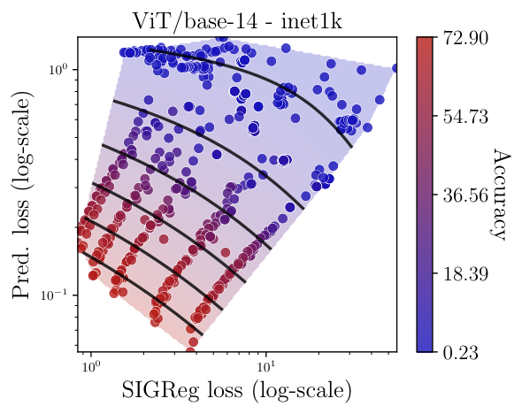
Figure 10: (SIGReg, prediction loss) -plane with downstream task accuracy shown with colors from blue (low) to red (high). We clearly observe that within this plane, there exists trade-off fronts between the two terms of LeJEPA producing similar downstream performance corresponding to different values of . Yet, those fronts are linear and pointed towards the lower left corner, i.e., LeJEPA’s training loss informs of downstream test performance across models and datasets (columns). Additional models and datasets provided in Figure21.Figure 11: Spearman correlation (y-axis) between LeJEPA’s training loss and downstream accuracy on the dataset’s classification task with a frozen backbone and linear evaluation. The x-axis varies in Equation10 following our scaling law of the loss w.r.t. . Using recovers the plain training loss. We clearly observe a very high correlation already for , which further increases up to for . The entire set of points is obtained across numerous hyper-parameters such as learning rate, weight decay, number of epochs, –demonstrating how LeJEPA’s training loss is strongly predictive of downstream performance which can be used for label-free cross-validation.Equation 10
(10)
6.3 In-Domain LeJEPA Outperforms Frontier Model Transfer Learning
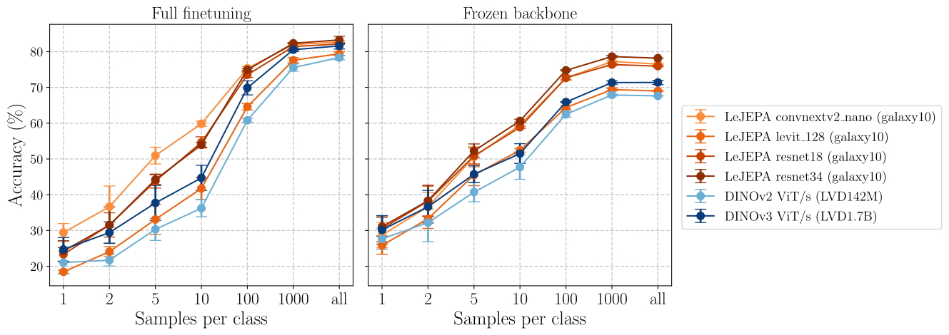
On Galaxy10, pretraining directly on the target visual domain with the proposed recipe can outperform transferring the selected natural-image foundation models. The comparison supports the value of in-domain pretraining under these budgets; it does not isolate the objective from every difference in data and model history.
Figure 12: Small architecture in-domain (Galaxy10) LeJEPA pretraining with linear probe evaluation using frozen backbone or full finetuning (columns) and with varying number of samples per class (x-axis). We compare against state-of-the-art foundation models (DINOv2/v3, IJEPA) over different random seeds. We observe that LeJEPA enables in-domain pretraining out of the box across architectures and able to outperform frontier foundation models. Corresponding numbers are provided in Table3.
Table 2: Few-shot classification accuracy (percentages) on 8 datasets spanning textures, objects, and fine-grained categories. Our LeJEPA achieves superior performance on fine-grained tasks (DTD, flowers102, food101) while requiring only 100 pretraining epochs compared to I-JEPA’s 300 epochs—a 3× reduction in training time and computational resources without sacrificing downstream task performance. This efficiency gain is particularly valuable for practical applications where training budget is limited. Bold indicates best performance within the IN-1K comparison group, all numbers are percentages.
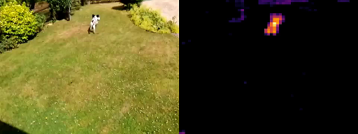
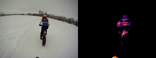
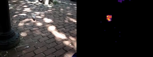
Figure 13: Emergent Object Segmentation via Last Layer Thresholding.LeJEPA naturally learns to segment and track salient objects (shown in attention maps on the right of each video) without explicit supervision. The results display impressive visual quality and strong temporal consistency across video frames (videos provided on our project page). This emergent capability demonstrates the rich semantic representations learned through our self-supervised approach.
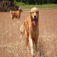
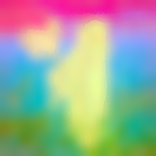
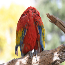
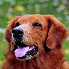
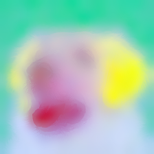
Figure 14: LeJEPA learns rich semantic representations through self-supervised learning.PCA visualization of last-layer features from LeJEPA (ViT-Large, 100 epochs on ImageNet-1K). For each image, features are independently projected to RGB using the first 3 principal components. Without any supervision, LeJEPA spontaneously develops semantically meaningful representations: notice how warm colors (red/magenta/pink) consistently capture foreground objects (parrot bodies, dog face), while cool colors (cyan/green/yellow) represent backgrounds and foliage. This emergent object-background separation and perceptual grouping discovered the visual structure of the world purely from unlabeled data.
ImageNet experiments scale encoder families and compare transfer with I-JEPA variants. Results show that the method can train larger backbones under the stated schedule. Parameter count, training duration, data and evaluation protocol should remain attached to any claimed advantage.
6.5 Emergent Semantic Structure in LeJEPA Representations
Attention and principal-component visualizations show foreground and semantic structure. Thresholded attention also produces temporally coherent masks in selected video examples without segmentation supervision. These qualitative demonstrations are not a complete quantitative video-segmentation benchmark.
7 Conclusion
LeJEPA offers an explicit, scalable alternative for collapse prevention and a theory-informed implementation. Useful semantics still depend on the views, data and predictive task. This makes the slow-feature counterexample and the later world-model-identifiability paper helpful companion readings.
Acknowledgments
The authors acknowledge feedback from Mike Rabbat and Lucas Maes.
Appendix A Additional Details on Nonlinear Probing
The neighbor-probe analysis averages labels in a radius around a query. Density smoothness, bounded derivatives and a smooth target function permit local expansions of bias. These conditions explain why the argument is more specific than a claim about arbitrary language or vision labels.
and the isotropic Gaussian is the unique minimizer of the integrated square bias. (Proof in SectionB.4.)
A.2 Kernel Probing
Kernel regression uses distance-weighted label averages instead of a hard neighborhood. The derivation adds tail and regularity assumptions and constrains embedding spread before comparing density shapes. The retained statements specify the optimization problem to which Gaussian optimality applies.
and the integrated variance is independent of .
Among all densities on with total-variance constrained, e.g., , the isotropic Gaussian is the unique minimizer. (Proof in SectionB.7.)
Appendix B Proofs
B.1 Proof of Section 3.1
The ridge-regression proof identifies a target direction aligned with a small covariance eigenvalue. Under equal total variance, anisotropy can increase shrinkage bias in that unfavorable direction. The argument is about a controlled worst-case comparison.
Equations 11–13
(11)
(12)
(13)
B.2 Proof of Section 3.1
For the unregularized estimator, the proof expresses total parameter variance through inverse covariance eigenvalues. Convexity shows why an equal spread minimizes this quantity under the stated fixed-sum constraint.
Equations
B.3 Proof of Section A.1
Local Taylor expansions of target and embedding density inside a small ball produce the neighbor estimator’s leading bias terms. Neighborhood symmetry removes odd-order contributions; the small-radius assumptions control the remainder.
Equations
B.4 Proof of Section A.1
The squared-bias calculation separates the density score, target gradient and target curvature. It averages over a specified isotropic prior on target gradients, an important assumption behind the resulting distribution preference.
Equations 14–15
(14)
(15)
1) The score-gradient term 𝔼 [ A ( X ) 2 ] .
The density-score contribution becomes a Fisher-information functional after averaging over the isotropic target-gradient prior.
Equation
2) The cross term 2 𝔼 [ A ( X ) C ( X ) ] .
The cross term is controlled using the stated symmetry and target-function assumptions. Its treatment cannot be assumed unchanged for an arbitrary downstream target family.
Equations
3) The curvature term 𝔼 [ C ( X ) 2 ] .
The remaining term measures target curvature. It separates a target-dependent contribution from the density-dependent part being optimized.
Equation
Putting it together.
Combining the terms shows which part of the approximation error can be improved by changing the embedding density under this model.
Equations
Lemma 6: Special case: Recovery of VCReg
Let be a mean-zero probability density on with covariance . Then
Equation
with equality if and only if .
Equation
Step 2: Optimizing over covariance shapes under scalar constraints
The next step compares allowable covariance shapes under different scalar constraints. The constraint determines what it means to compare distributions with the same available spread.
Equation
(a) Trace constraint.
With fixed covariance trace, the argument favors equal variance across coordinates through a convexity bound.
Equations
(b) Determinant constraint.
The determinant-constrained case fixes a volume-related quantity and analyzes the corresponding covariance optimum.
Equations
(c) Frobenius-norm constraint.
The Frobenius-norm case constrains the squared size of the covariance matrix before comparing its eigenvalues.
Equations
(d) Spectral-radius constraint.
The spectral-radius case restricts the largest covariance eigenvalue. It is a different feasible set from fixing total variance.
Equations
Conclusion: Isotropic Gaussian is optimal
The Gaussian and isotropic conclusions combine density and covariance optimization under the stated assumptions. They do not prove that every semantically useful representation must be identical to this optimum.
Theorem 9: Special case: Recovery of VCReg
Fix one of the following scalar covariance constraints for a mean-zero distribution on :
•
trace: ,
•
determinant: ,
•
Frobenius norm: ,
•
spectral radius upper bound: .
Then the Fisher-information functional is minimized over all such by the isotropic Gaussian with chosen to satisfy the constraint. The minimal values are:
Equation
In each case, is the unique minimizer (up to null sets).
B.5 Proof of Section A.2
The kernel-probe proof repeats the local bias/variance analysis with kernel-weighted neighborhoods and its stated smoothness and tail conditions.
Equations
B.6 Proof of Equation 6 to Equation 7
This calculation relates the characteristic-function discrepancy to the expression used by the proposed regularizer. The exact algebraic expressions are preserved.
The remaining kernel-probe argument compares admissible embedding densities under the specified constraints, completing the conditional optimality result.
Equations
B.8 Proof of Section 4.1
The projection argument uses uniqueness of characteristic functions: agreement of every one-dimensional projected law identifies the full joint law. It is a population statement requiring every direction, before finite testing is considered.
The consistency argument assumes sufficiently dense direction coverage and a detectable neighborhood around a separating direction. These assumptions connect projection-wise tests to an eventual full-distribution decision.
Equations
B.10 Proof of Section 4.3
The finite-direction approximation bound uses smoothness and quasi-uniform coverage of the sphere. Its dimension and regularity dependence should be kept when interpreting the practical projection count.
Equations
B.11 Proof of Section 4.2.1
A linear-algebra construction makes two distinct discrete distributions agree on any prescribed finite set of moments. This explains why low-order moment matching alone cannot identify a general distribution.
B.12 Proof of Section 4.2.3
Bounded complex exponentials yield bounds on the chosen loss derivatives, while moment penalties can grow polynomially with sample magnitude. The bounds concern the statistic and its weighting scale, not every component of a full neural-network optimizer.
Equations
B.13 Proof of Section 5.1
Expanding the empirical characteristic-function square isolates the minibatch bias. Sampling bias and deterministic quadrature error are separate quantities; rescaling the integration grid does not remove the former automatically.
The argument derives the mean and covariance conditions obtained when projected first and second moments match the target in every direction.
Part I: 𝔼 [ 𝐗 ] = 𝟎
Zero mean in every projected direction implies the full embedding mean vector is zero.
Equations 35–39
(35)
(36)
(37)
(38)
(39)
Part II: Cov ( 𝐗 ) = 𝐈 d
Unit variance along coordinate axes fixes diagonal covariance entries; combined-axis directions then force off-diagonal entries to zero. This recovers identity covariance, which alone does not identify a Gaussian density.
Equations 40–50
(40)
(41)
(42)
(43)
(44)
(45)
(46)
(47)
(48)
(49)
(50)
Appendix C Background
The background appendix derives ordinary least squares from a linear model and its normal equations, making explicit the invertibility and noise assumptions used in the probe discussion.
Equations 51
(51)
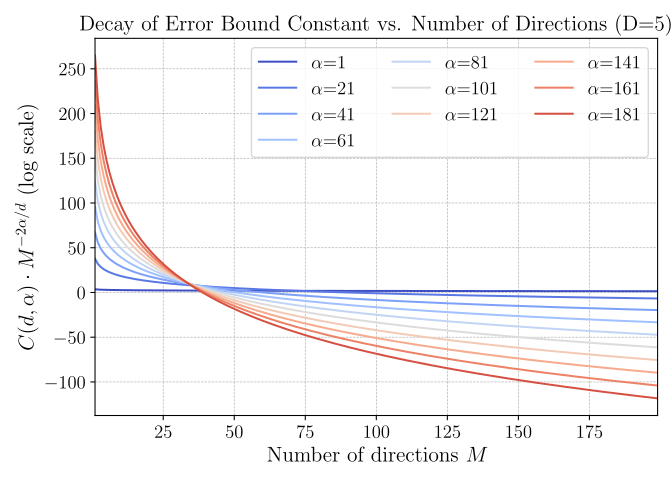
Figure 15: Depiction of the expected BCS loss upper bound (Section4.3) for various smoothness values . We clearly see that as the smoothness increases (blue to red), as the upper bound decreases more and more rapidly with .
Figure 16: Reprise of Figure6 for additional dimensions and number of 1d projections.
Figure 17: Depiction of the distribution of optimized values from OLS when comparing and from Sections3.1 and 3.1. We clearly observe that the anisotropic version (blue) provides much lower variance compared to the isotropic case (red). We consider a binary classification (linear separable class) (top row), a linear regression task (middle row), and a nonlinear regression task with smooth targets (bottom row). For each case, we resample the training samples numerous times and produce an estimate for each time. Because the data is -dimensional, we can visualize the distribution directly.
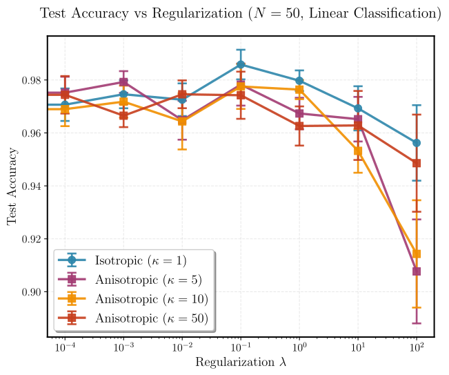
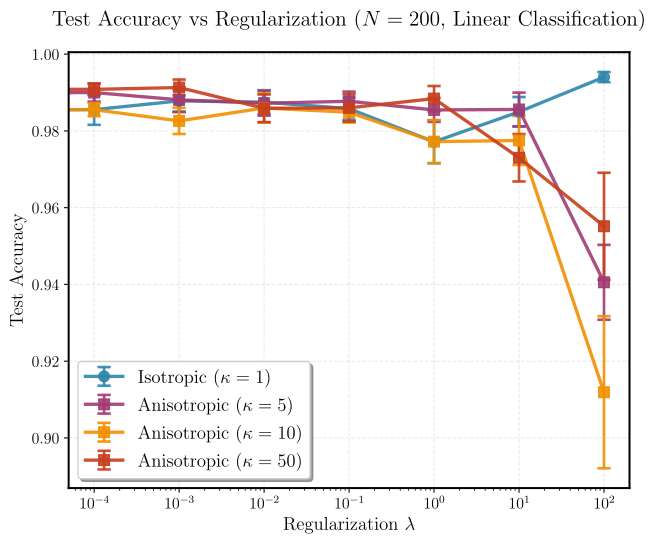
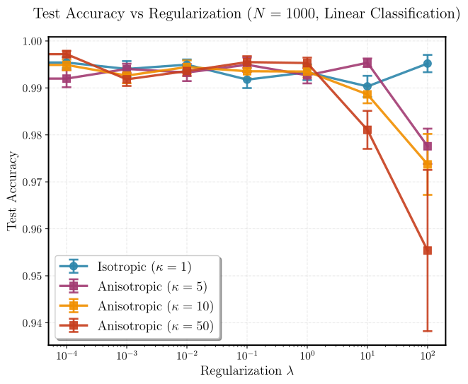
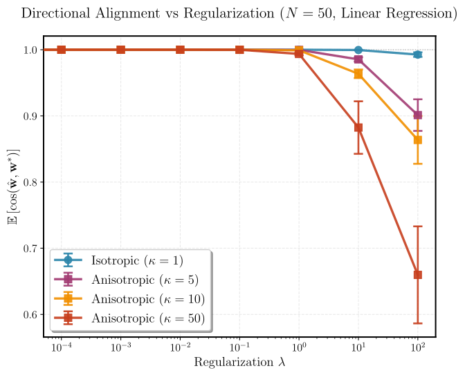
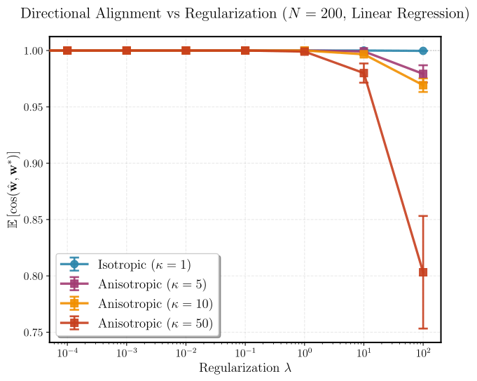
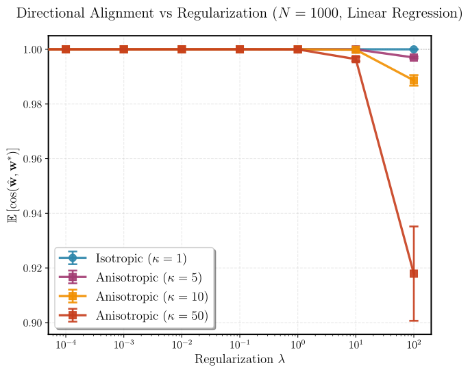
Figure 18: Depiction of accuracy (top) and cosine similarity between estimated and true estimator (bottom) for the OLS setting with varying strength of Tikhonov regularization (x-axis) comparing isotropic and anisotropic embeddings. As per Section5.1, the anisotropic distribution creates a bias in the OLS estimation for nonzero regularization.
Figure 19: Additional figures provides in Figure19
Table 3: Performance metrics across different sample sizes from Figure12
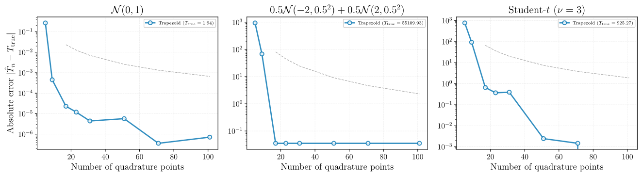
Figure 20: Proposed trapezoid quadrature for the Epps-Pulley statistic as implemented in . We depict the approximation error of the integral for various distributions, demonstrate rapid convergence (faster than quadratic show in grey line) across possible embedding distributions.
Table 5: Small architecture in-domain LeJEPA pretraining from random initialization across datasets and architectures, with frozen backbone linear evaluation. First, LeJEPA is able to produce near state-of-the-art performances on tiny dataset with only a thousand samples, e.g., flowers102. Second, on non-natural image data, LeJEPA clearly outperforms the latest frontier vision models, e.g., Galaxy10. See Figure12 for additional experiments with varying number of training samples and with full finetuning.
Table 6: Time (in millisecond) to compute the proposed SIGReg loss from on a Tesla V100-SXM2-16GB for varying mini-batch size (), number of slices (), integration points. Results are computed over runs.
A Sobol sequence is transformed into approximate sphere directions through Gaussian quantiles and normalization. This aims for more even directional coverage; the nonlinear mapping need not preserve the original discrepancy guarantee exactly.
Appendix E Shapiro-Wilk Test
This appendix reviews Shapiro–Wilk-style normality statistics and approximations. It supplies context for the paper’s decision not to use an order-statistic-based training penalty.
Equations 52–58
(52)
(53)
(54)
(55)
(56)
(57)
(58)
Appendix F Multivariate Statistics
The final appendix lists multivariate characteristic-function, moment-generating-function and moment tests. Their formulas clarify the alternatives and their computational costs; they are not all implemented as the default SIGReg objective.
Equations 59–68
(59)
(60)
(61)
(62)
(63)
(64)
(65)
(66)
(67)
(68)
121 references
Abu Alfeilat et al. (2019)H. A. Abu Alfeilat, A. B. Hassanat, O. Lasassmeh, A. S. Tarawneh, M. B. Alhasanat, H. S. Eyal Salman, and V. S. PrasathEffects of distance measure choice on k-nearest neighbor classifier performance: a review.
Big data7 (4), pp. 221–248.
Agrawal et al. (2022)K. K. Agrawal, A. K. Mondal, A. Ghosh, and B. RichardsA-req: assessing representation quality in self-supervised learning by measuring eigenspectrum decay.
Advances in Neural Information Processing Systems35, pp. 17626–17638.
Anderson and Darling (1952)T. W. Anderson and D. A. DarlingAsymptotic theory of certain" goodness of fit" criteria based on stochastic processes.
The annals of mathematical statistics, pp. 193–212.
Assran et al. (2022)M. Assran, R. Balestriero, Q. Duval, F. Bordes, I. Misra, P. Bojanowski, P. Vincent, M. Rabbat, and N. BallasThe hidden uniform cluster prior in self-supervised learning.
arXiv preprint arXiv:2210.07277.
Assran et al. (2023)M. Assran, Q. Duval, I. Misra, P. Bojanowski, P. Vincent, M. Rabbat, Y. LeCun, and N. BallasSelf-supervised learning from images with a joint-embedding predictive architecture.
In Proceedings of the IEEE/CVF Conference on Computer Vision and Pattern Recognition,
pp. 15619–15629.
Balestriero et al. (2025)R. Balestriero, N. Ballas, M. Rabbat, and Y. LeCunGaussian embeddings: how jepas secretly learn your data density.
arXiv preprint arXiv:2510.05949.
Balestriero et al. (2023)R. Balestriero, M. Ibrahim, V. Sobal, A. Morcos, S. Shekhar, T. Goldstein, F. Bordes, A. Bardes, G. Mialon, Y. Tian, et al.A cookbook of self-supervised learning.
arXiv preprint arXiv:2304.12210.
Balestriero and LeCun (2022)R. Balestriero and Y. LeCunContrastive and non-contrastive self-supervised learning recover global and local spectral embedding methods.
Advances in Neural Information Processing Systems35, pp. 26671–26685.
Balestriero and LeCun (2024)R. Balestriero and Y. LeCunLearning by reconstruction produces uninformative features for perception.
arXiv preprint arXiv:2402.11337.
Bar et al. (2023)A. Bar, F. Bordes, A. Shocher, M. Assran, P. Vincent, N. Ballas, T. Darrell, A. Globerson, and Y. LeCunStochastic positional embeddings improve masked image modeling.
arXiv preprint arXiv:2308.00566.
Bardes et al. (2021)A. Bardes, J. Ponce, and Y. LeCunVicreg: variance-invariance-covariance regularization for self-supervised learning.
arXiv preprint arXiv:2105.04906.
Beirlant et al. (1997)J. Beirlant, E. J. Dudewicz, L. Györfi, E. C. Van der Meulen, et al.Nonparametric entropy estimation: an overview.
International Journal of Mathematical and Statistical Sciences6 (1), pp. 17–39.
Bonneel et al. (2015)N. Bonneel, J. Rabin, G. Peyré, and H. PfisterSliced and radon wasserstein barycenters of measures.
Journal of Mathematical Imaging and Vision51 (1), pp. 22–45.
Bromley et al. (1993)J. Bromley, I. Guyon, Y. LeCun, E. Säckinger, and R. ShahSignature verification using a" siamese" time delay neural network.
Advances in neural information processing systems6.
Caron et al. (2021)M. Caron, H. Touvron, I. Misra, H. Jégou, J. Mairal, P. Bojanowski, and A. JoulinEmerging properties in self-supervised vision transformers.
In Proceedings of the IEEE/CVF international conference on computer vision,
pp. 9650–9660.
Chen et al. (2020a)T. Chen, S. Kornblith, M. Norouzi, and G. HintonA simple framework for contrastive learning of visual representations.
In International conference on machine learning,
pp. 1597–1607.
Chen et al. (2020b)T. Chen, S. Kornblith, K. Swersky, M. Norouzi, and G. E. HintonBig self-supervised models are strong semi-supervised learners.
Advances in neural information processing systems33, pp. 22243–22255.
Chen et al. (2021)X. Chen, S. Xie, and K. HeAn empirical study of training self-supervised vision transformers.
In Proceedings of the IEEE/CVF international conference on computer vision,
pp. 9640–9649.
Chwialkowski et al. (2016)K. Chwialkowski, H. Strathmann, and A. GrettonA kernel test of goodness of fit.
In International conference on machine learning,
pp. 2606–2615.
Cosentino et al. (2022)R. Cosentino, A. Sengupta, S. Avestimehr, M. Soltanolkotabi, A. Ortega, T. Willke, and M. TepperToward a geometrical understanding of self-supervised contrastive learning.
arXiv preprint arXiv:2205.06926.
Cramér (1928)H. CramérOn the composition of elementary errors: first paper: mathematical deductions.
Scandinavian Actuarial Journal1928 (1), pp. 13–74.
Cuturi et al. (2019)M. Cuturi, O. Teboul, and J. VertDifferentiable ranking and sorting using optimal transport.
Advances in neural information processing systems32.
Dick and Pillichshammer (2010)J. Dick and F. PillichshammerDigital nets and sequences: discrepancy theory and quasi–monte carlo integration.
Cambridge University Press.
Ermolov et al. (2021)A. Ermolov, A. Siarohin, E. Sangineto, and N. SebeWhitening for self-supervised representation learning.
In International conference on machine learning,
pp. 3015–3024.
Fan et al. (2025)D. Fan, S. Tong, J. Zhu, K. Sinha, Z. Liu, X. Chen, M. Rabbat, N. Ballas, Y. LeCun, A. Bar, et al.Scaling language-free visual representation learning.
arXiv preprint arXiv:2504.01017.
Garrido et al. (2023)Q. Garrido, R. Balestriero, L. Najman, and Y. LecunRankme: assessing the downstream performance of pretrained self-supervised representations by their rank.
In International conference on machine learning,
pp. 10929–10974.
Golub et al. (1999)G. H. Golub, P. C. Hansen, and D. P. O’LearyTikhonov regularization and total least squares.
SIAM journal on matrix analysis and applications21 (1), pp. 185–194.
Goyal et al. (2019)P. Goyal, D. Mahajan, A. Gupta, and I. MisraScaling and benchmarking self-supervised visual representation learning.
In Proceedings of the ieee/cvf International Conference on computer vision,
pp. 6391–6400.
Gregory (1980)R. L. GregoryPerceptions as hypotheses.
Philosophical Transactions of the Royal Society of London. B, Biological Sciences290 (1038), pp. 181–197.
Gretton et al. (2012)A. Gretton, K. M. Borgwardt, M. J. Rasch, B. Schölkopf, and A. SmolaA kernel two-sample test.
The journal of machine learning research13 (1), pp. 723–773.
Grill et al. (2020)J. Grill, F. Strub, F. Altché, C. Tallec, P. Richemond, E. Buchatskaya, C. Doersch, B. Avila Pires, Z. Guo, M. Gheshlaghi Azar, et al.Bootstrap your own latent-a new approach to self-supervised learning.
Advances in neural information processing systems33, pp. 21271–21284.
Grover et al. (2019)A. Grover, E. Wang, A. Zweig, and S. ErmonStochastic optimization of sorting networks via continuous relaxations.
arXiv preprint arXiv:1903.08850.
Gutmann and Hyvärinen (2010)M. Gutmann and A. HyvärinenNoise-contrastive estimation: a new estimation principle for unnormalized statistical models.
In Proceedings of the thirteenth international conference on artificial intelligence and statistics,
pp. 297–304.
Hammersley and Morton (1954)J. Hammersley and K. MortonThe estimation of location and scale parameters from grouped data.
Biometrika41 (3/4), pp. 296–301.
He et al. (2020)K. He, H. Fan, Y. Wu, S. Xie, and R. GirshickMomentum contrast for unsupervised visual representation learning.
In Proceedings of the IEEE/CVF conference on computer vision and pattern recognition,
pp. 9729–9738.
Hjelm et al. (2018)R. D. Hjelm, A. Fedorov, S. Lavoie-Marchildon, K. Grewal, P. Bachman, A. Trischler, and Y. BengioLearning deep representations by mutual information estimation and maximization.
arXiv preprint arXiv:1808.06670.
Hoare (1962)C. A. R. HoareQuicksort.
The Computer Journal5 (1), pp. 10–16.
External Links: ISSN 0010-4620,
Document,
Link,
https://academic.oup.com/comjnl/article-pdf/5/1/10/1111445/050010.pdf
Izmailov et al. (2019)P. Izmailov, D. Podoprikhin, T. Garipov, D. Vetrov, and A. G. WilsonAveraging weights leads to wider optima and better generalization.
External Links: 1803.05407,
Link
Jarque and Bera (1980)C. M. Jarque and A. K. BeraEfficient tests for normality, homoscedasticity and serial independence of regression residuals.
Economics letters6 (3), pp. 255–259.
Jing et al. (2021)L. Jing, P. Vincent, Y. LeCun, and Y. TianUnderstanding dimensional collapse in contrastive self-supervised learning.
arXiv preprint arXiv:2110.09348.
Joe (1989)H. JoeEstimation of entropy and other functionals of a multivariate density.
Annals of the Institute of Statistical Mathematics41 (4), pp. 683–697.
Kerdreux et al. (2025)T. Kerdreux, A. Tuel, Q. Febvre, A. Mouche, and B. ChapronEfficient self-supervised learning for earth observation via dynamic dataset curation.
In Proceedings of the Computer Vision and Pattern Recognition Conference,
pp. 3017–3027.
Khazatsky et al. (2024)A. Khazatsky, K. Pertsch, S. Nair, A. Balakrishna, S. Dasari, S. Karamcheti, S. Nasiriany, M. K. Srirama, L. Y. Chen, K. Ellis, et al.Droid: a large-scale in-the-wild robot manipulation dataset.
arXiv preprint arXiv:2403.12945.
Kingma et al. (2014)D. P. Kingma, D. J. Rezende, S. Mohamed, and M. WellingSemi-supervised learning with deep generative models.
Advances in neural information processing systems27.
Kolmogorov (1933)A. N. KolmogorovSulla determinazione empirica di una legge di distribuzione.
Giornale dell’Istituto Italiano degli Attuari4, pp. 83–91.
Liu et al. (2021)X. Liu, F. Zhang, Z. Hou, L. Mian, Z. Wang, J. Zhang, and J. TangSelf-supervised learning: generative or contrastive.
IEEE transactions on knowledge and data engineering35 (1), pp. 857–876.
Ma and Collins (2018)Z. Ma and M. CollinsNoise contrastive estimation and negative sampling for conditional models: consistency and statistical efficiency.
arXiv preprint arXiv:1809.01812.
Maltenberger et al. (2022)T. Maltenberger, I. Ilic, I. Tolovski, and T. RablEvaluating multi-gpu sorting with modern interconnects.
In Proceedings of the 2022 International Conference on Management of Data,
pp. 1795–1809.
Masson et al. (2019)C. Masson, J. E. Rim, and H. K. LeeDdsketch: a fast and fully-mergeable quantile sketch with relative-error guarantees.
arXiv preprint arXiv:1908.10693.
McAllester and Stratos (2020)D. McAllester and K. StratosFormal limitations on the measurement of mutual information.
In International Conference on Artificial Intelligence and Statistics,
pp. 875–884.
Mhaskar et al. (2001)H. Mhaskar, F. Narcowich, and J. WardSpherical marcinkiewicz-zygmund inequalities and positive quadrature.
Mathematics of computation70 (235), pp. 1113–1130.
Miller (2003)E. G. MillerA new class of entropy estimators for multi-dimensional densities.
In 2003 IEEE International Conference on Acoustics, Speech, and Signal Processing, 2003. Proceedings.(ICASSP’03).,
Vol. 3, pp. III–297.
Narcowich et al. (2006)F. J. Narcowich, P. Petrushev, and J. D. WardLocalized tight frames on spheres.
SIAM Journal on Mathematical Analysis38 (2), pp. 574–594.
Neyman and Pearson (1933)J. Neyman and E. S. PearsonIX. on the problem of the most efficient tests of statistical hypotheses.
Philosophical Transactions of the Royal Society of London. Series A, Containing Papers of a Mathematical or Physical Character231 (694-706), pp. 289–337.
Oquab et al. (2023)M. Oquab, T. Darcet, T. Moutakanni, H. Vo, M. Szafraniec, V. Khalidov, P. Fernandez, D. Haziza, F. Massa, A. El-Nouby, et al.Dinov2: learning robust visual features without supervision.
arXiv preprint arXiv:2304.07193.
Papyan et al. (2020)V. Papyan, X. Han, and D. L. DonohoPrevalence of neural collapse during the terminal phase of deep learning training.
Proceedings of the National Academy of Sciences117 (40), pp. 24652–24663.
Poole et al. (2019)B. Poole, S. Ozair, A. Van Den Oord, A. Alemi, and G. TuckerOn variational bounds of mutual information.
In International conference on machine learning,
pp. 5171–5180.
Rahman and Govindarajulu (1997)M. M. Rahman and Z. GovindarajuluA modification of the test of shapiro and wilk for normality.
Journal of Applied Statistics24 (2), pp. 219–236.
Rodas et al. (2025)B. Rodas, N. Montesino, J. Ambsdorf, D. Klindt, and R. BalestrieroDIET-cp: lightweight and data efficient self supervised continued pretraining.
arXiv preprint arXiv:2509.06990.
Roy (1953)S. N. RoyOn a heuristic method of test construction and its use in multivariate analysis.
The Annals of Mathematical Statistics24 (2), pp. 220–238.
Rumelhart et al. (1986)D. E. Rumelhart, G. E. Hinton, and R. J. WilliamsLearning representations by back-propagating errors.
nature323 (6088), pp. 533–536.
Shapiro and Francia (1972)S. S. Shapiro and R. FranciaAn approximate analysis of variance test for normality.
Journal of the American statistical Association67 (337), pp. 215–216.
Shwartz Ziv and LeCun (2024)R. Shwartz Ziv and Y. LeCunTo compress or not to compress—self-supervised learning and information theory: a review.
Entropy26 (3), pp. 252.
Shwartz-Ziv et al. (2022)R. Shwartz-Ziv, R. Balestriero, and Y. LeCunWhat do we maximize in self-supervised learning?.
arXiv preprint arXiv:2207.10081.
Siméoni et al. (2025)O. Siméoni, H. V. Vo, M. Seitzer, F. Baldassarre, M. Oquab, C. Jose, V. Khalidov, M. Szafraniec, S. Yi, M. Ramamonjisoa, et al.Dinov3.
arXiv preprint arXiv:2508.10104.
Song et al. (2020)Y. Song, S. Garg, J. Shi, and S. ErmonSliced score matching: a scalable approach to density and score estimation.
In Uncertainty in artificial intelligence,
pp. 574–584.
Sriperumbudur et al. (2010)B. K. Sriperumbudur, A. Gretton, K. Fukumizu, B. Schölkopf, and G. R. LanckrietHilbert space embeddings and metrics on probability measures.
The Journal of Machine Learning Research11, pp. 1517–1561.
Sun and Huang (2010)S. Sun and R. HuangAn adaptive k-nearest neighbor algorithm.
In 2010 seventh international conference on fuzzy systems and knowledge discovery,
Vol. 1, pp. 91–94.
Tanasic et al. (2013)I. Tanasic, L. Vilanova, M. Jordà, J. Cabezas, I. Gelado, N. Navarro, and W. HwuComparison based sorting for systems with multiple gpus.
In Proceedings of the 6th Workshop on General Purpose Processor Using Graphics Processing Units,
pp. 1–11.
Taunk et al. (2019)K. Taunk, S. De, S. Verma, and A. SwetapadmaA brief review of nearest neighbor algorithm for learning and classification.
In 2019 international conference on intelligent computing and control systems (ICCS),
pp. 1255–1260.
Thilak et al. (2023)V. Thilak, C. Huang, O. Saremi, L. Dinh, H. Goh, P. Nakkiran, J. M. Susskind, and E. LittwinLidar: sensing linear probing performance in joint embedding ssl architectures.
arXiv preprint arXiv:2312.04000.
Tian et al. (2020)Y. Tian, C. Sun, B. Poole, D. Krishnan, C. Schmid, and P. IsolaWhat makes for good views for contrastive learning?.
Advances in neural information processing systems33, pp. 6827–6839.
Tian et al. (2021)Y. Tian, X. Chen, and S. GanguliUnderstanding self-supervised learning dynamics without contrastive pairs.
In International Conference on Machine Learning,
pp. 10268–10278.
Van Assel et al. (2025)H. Van Assel, M. Ibrahim, T. Biancalani, A. Regev, and R. BalestrieroJoint embedding vs reconstruction: provable benefits of latent space prediction for self supervised learning.
arXiv preprint arXiv:2505.12477.
Vincent et al. (2010)P. Vincent, H. Larochelle, I. Lajoie, Y. Bengio, P. Manzagol, and L. BottouStacked denoising autoencoders: learning useful representations in a deep network with a local denoising criterion..
Journal of machine learning research11 (12).
Vo et al. (2024)H. V. Vo, V. Khalidov, T. Darcet, T. Moutakanni, N. Smetanin, M. Szafraniec, H. Touvron, C. Couprie, M. Oquab, A. Joulin, et al.Automatic data curation for self-supervised learning: a clustering-based approach.
arXiv preprint arXiv:2405.15613.
Wang et al. (2022)X. Wang, H. Fan, Y. Tian, D. Kihara, and X. ChenOn the importance of asymmetry for siamese representation learning.
In Proceedings of the IEEE/CVF conference on computer vision and pattern recognition,
pp. 16570–16579.
Weisburg and Binham (1975)S. Weisburg and C. BinhamAn approximate analysis of variance test for non-normality suitable for machine computation.
Technometrics17, pp. 133–134.
Zhang et al. (2017)S. Zhang, X. Li, M. Zong, X. Zhu, and R. WangEfficient knn classification with different numbers of nearest neighbors.
IEEE transactions on neural networks and learning systems29 (5), pp. 1774–1785.
Zhang et al. (2023)Y. Zhang, Z. Tan, J. Yang, W. Huang, and Y. YuanMatrix information theory for self-supervised learning.
arXiv preprint arXiv:2305.17326.



 dimension=128, slices=100
 dimension=1024, slices=100