At a glance
This edition reviews arXiv v2 dated 11 September 2026. The ten authors are affiliated with Carnegie Mellon, Maryland and Pennsylvania. All mathematical programs, numbered equations, figures, algorithm steps and references are retained.
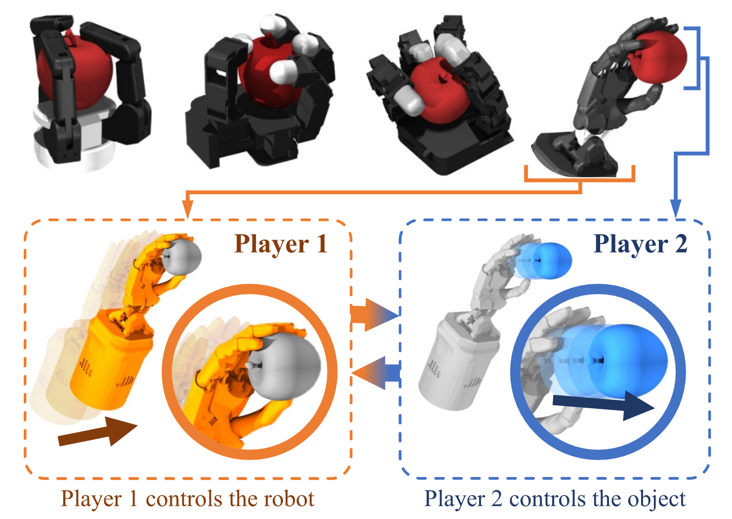
Game4Grasp alternates between a hand that seeks a feasible enclosing grasp and an adversarial object that seeks a collision-free escape motion. Both players solve constrained local optimization problems using geometric point-set models.
Simulation success averages 75.78%, versus 68.27% for D(R,O), a 7.51-percentage-point gain; the largest hand-specific gain is 19.61 points on ShadowHand. Hardware trials achieve 34/40 on ShadowHand and 35/40 on LEAP Hand. These empirical results do not establish a general convergence or force-closure guarantee. Code accompanies the paper.
I Introduction
A geometrically plausible hand pose may still let an object escape under disturbance. The paper makes this escape search part of synthesis: an adversarial object motion challenges the current hand configuration, and the hand responds by constraining that motion.
The method combines a kinematic grasp condition with alternating augmented-Lagrangian optimization. It requires object geometry and pose and tests simulated disturbance resistance, a continuously changing mesh example and real static holding. Broader tool use and adaptive manipulation remain proposed applications.
II Related Works
Related work separates adversarial robustness tests from geometric and wrench-based definitions of a secure grasp.
II-A Adversarial Approaches in Dexterous Grasp Synthesis
Prior grasp attacks, adversarial object sets and domain-adversarial visual training expose weaknesses or improve representations. Here the adversary directly optimizes object motion within the grasp-generation loop.
II-B Conditions for Firm Grasp
Form closure excludes feasible object motion through contact geometry; caging restricts the object to a bounded connected region; force closure asks whether contact wrenches can oppose external loads. The proposed condition is geometric and friction-free, closer to form closure than a force-balance certificate.
A collision indicator allows gradient-based optimization without explicitly enumerating contact points. It still depends on sampled object geometry and approximate hand collision volumes; avoiding explicit contact identification does not eliminate geometric uncertainty.
III Grasp Synthesis as a Two-Player Game
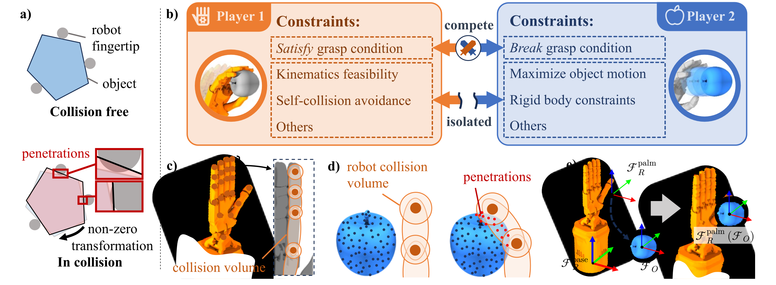
The hand has a floating base and M joints. The method represents its state and the rigid object pose, defines a local no-escape condition, and gives the hand and object opposing constrained objectives.
Equation
III-A Firm Grasp Condition
The intended condition is collision-free placement at the original pose and penetration under every sufficiently small nonzero object displacement. A six-dimensional twist parameterizes the rigid transformation. The two original conditions appear below.
Equation 1b prints all twists with magnitude below ε without explicitly excluding zero; literally including zero conflicts with Equation 1a. The surrounding prose specifies nonzero motions and supplies the intended interpretation. Small bounds restrict the local search and avoid some large symmetry-equivalent poses, but cannot remove continuous infinitesimal symmetry such as rotating an ideal cylinder about its axis.
This is a local geometric condition, not a frictional stability guarantee or a proof that a finite sampled optimizer has ruled out every escape direction.
Equations 1a–1b
| (1a) | ||||
| (1b) | ||||
III-B Two-Player Game Formulation
Player 1 minimizes a fingertip-contact objective while enforcing kinematics, state bounds, self-collision avoidance, no initial penetration and blocking the current adversarial displacement. Player 2 maximizes the squared twist norm while staying within object-motion bounds and avoiding the fixed hand.
Alternating responses replace the impossible direct enumeration of infinitely many object transformations with repeated candidate escapes. The printed programs use non-strict inequalities at the boundary; approximate local responses do not certify the original universal strict condition.
Equation P1
|
Equation P2
|
III-C Objectives and Constraints
The object is sampled as N surface points and the hand represented by K frame-attached points. Pairwise distances encode kinematics, collision margins and fingertip proximity, following propagative distance optimization. The original point-set definitions are preserved below.
Equation
III-C 1 Robot kinematics constraints
Forward kinematics relates the hand state to its frame-attached points. A modified proximal Denavit–Hartenberg representation expresses constraints through distances instead of explicit trigonometric joint-angle relations, intended to ease local inverse kinematics. This reparameterization does not make the full grasp problem convex or guarantee a global solution.
Equation 2
| (2) |
III-C 2 Object point cloud constraints
Object points must be a single rigid transform of their initial cloud, as specified by Equation 3. The adversary changes pose rather than independently moving points or deforming the shape within each grasp solve.
Equation 3
| (3) |
III-C 3 Box constraints on robot states
A sigmoid maps unconstrained variables into joint/base bounds. Its range is the open interval between the limits, approximating the requested closed box while excluding exact endpoints. The original sigmoid definition and variable-domain notation are retained; the stated ω-domain combines Euclidean coordinates with SE(3) despite the componentwise mapping.
Equations 4
| (4) |
III-C 4 Box constraints on object transformations
The object’s six twist coordinates use the same sigmoid construction to stay between −ε and ε. These bounds define the searched disturbance neighborhood. The paper does not specify all bound values or a normalization reconciling translation and rotation in the squared twist objective.
Equation 5
| (5) |
III-C 5 Differentiable constraints related to robot-object collisions
A joint-center sphere uses point distance minus radius; a link ellipsoid uses the sum of distances to its endpoints minus a threshold. Penetration occurs when an object point lies inside a modeled hand volume.
The text groups pairwise terms into ψ without fully specifying the scalar/vector aggregation. Collision-free placement requires all relevant pair margins nonnegative, whereas existence of penetration requires at least one negative margin; that distinction matters when interpreting the opposing inequalities. Finite cloud sampling and simplified collision volumes also limit geometric fidelity.
Equations 6–8
| (6) |
| (7) |
| (8) |
III-C 6 Differentiable robot self-collision avoidance constraints
Self-collision constraints replace object points with other hand points and exclude identical points or link endpoints. The same sphere/ellipsoid distance model is reused. These formulas describe the chosen approximation rather than exact collision testing between every full hand-link mesh.
Equations 9–11
| (9) |
| (10) | ||||
| (11) |
III-C 7 Grasping objective function
For selected fingertip points, the objective measures nearest-object distance beyond a contact threshold, clips negative residuals to zero, and sums squared residuals. It encourages proximity but does not by itself resist escape; the adversarial constraints supply that role.
Nearest-point and max operations are piecewise smooth and can be nonsmooth at switches. The objective is geometric, with no explicit friction cone or contact-force optimization.
Equations 12–13
| (12) |
| (13) |
IV Algorithm
The players alternate local solves. Initialization aligns a manually defined palm frame with the object centroid and principal axes estimated by PCA. This provides one useful starting pose, but asymmetric or complex geometry can give a poor alignment.
IV-A Solving Inner Optimization Problems
Substituting the state mappings yields the transformed collision, self-collision and contact functions in Equations 14–16. Player 1 gathers its inequalities into C; Player 2 penalizes collision while maximizing admissible motion. The original C expression and both transformed programs remain below.
Augmented-Lagrangian objectives use positive-part violation penalties. Multipliers start at zero and penalties at one; L-BFGS minimizes the inner objective, then multipliers are updated and the penalty is multiplied by ten.
Each player stops on constraint tolerance, relative improvement below 10⁻², or its iteration cap. A stop caused by stagnation or a cap need not mean the constraints are satisfied. The paper does not supply a general global-convergence result or a complete multiplier-update equation.
Equations 14–16
| (14) |
| (15) |
| (16) |
Equation P1 †
|
Equation P2 †
|
Equations 17–18
| (17) |
| (18) | ||||
Equation 19
|
Equation 20
|
Equation
IV-B Solving the Game via Iterative Best Response Strategy
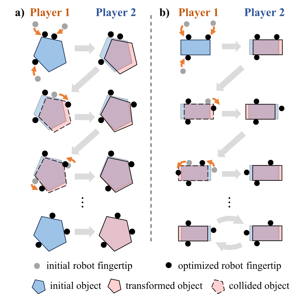
Player 1 updates first against the previous object displacement; Player 2 then searches for an escape against the new hand. A near-zero adversarial result suggests a locally immobilized object under this model, while infeasibility or local solver failure can create cycles.
A failed local escape search is not proof that no escape exists, and collapsing the collision inequalities to a contact boundary does not alone prove Player 1 cannot improve its objective. Figure 3 preserves both settling and cyclic examples.
Algorithm 1’s printed stopping test uses the signed difference ‖δᵗ‖−‖δᵗ⁻¹‖<ε′. A sufficiently decreasing norm therefore triggers it, even without stagnation; the prose instead discusses no significant progress over multiple iterations. The printed return variable is assigned only inside the early-stop branch, leaving iteration-cap behavior unspecified in the pseudocode. The original algorithm is retained unchanged in meaning.
Equations 21–22
| (21) |
| (22) |
V Experiments and Results
Experiments use a maximum of ten game iterations and one hundred inner iterations per player, constraint tolerances 10⁻⁵, escape-norm tolerance 10⁻³ and progress tolerance 10⁻⁵. These are termination settings, distinct from the object-motion box bounds.
V-A Our Approach vs. Baselines
Simulation compares disturbance-resistant grasps across three hands, then examines adversarial ablation and runtime.
V-A 1 Setup
CMapDataset supplies 58 objects. Barrett, Allegro and ShadowHand are evaluated in Isaac Gym, with a simple grasp controller from the D(R,O) work. Each object/method gets one hundred trials using randomly sampled point clouds.
Forces in six ±axis directions act for one second each. The base magnitude is 0.5 times object mass, equivalent to 0.5 m/s² acceleration under the stated units. Success means final displacement below 2 cm after all six perturbations, not necessarily a bound on every intermediate displacement or orientation change.
V-A 2 Baselines
D(R,O) is trained on 48 of the 58 objects; ten are held out. The proposed method requires no training examples, but evaluates the same supplied geometries. The headline full-set comparison includes the learned baseline’s training objects rather than reporting only its held-out split.
The Player1 ablation removes the object adversary while retaining contact, kinematic, bound and collision constraints. Its complete program is preserved below. This isolates the adversarial loop more directly than comparing against a separately trained representation.
Equation Baseline: Player1
| (Baseline: Player1) | ||||
V-A 3 Comparison Results
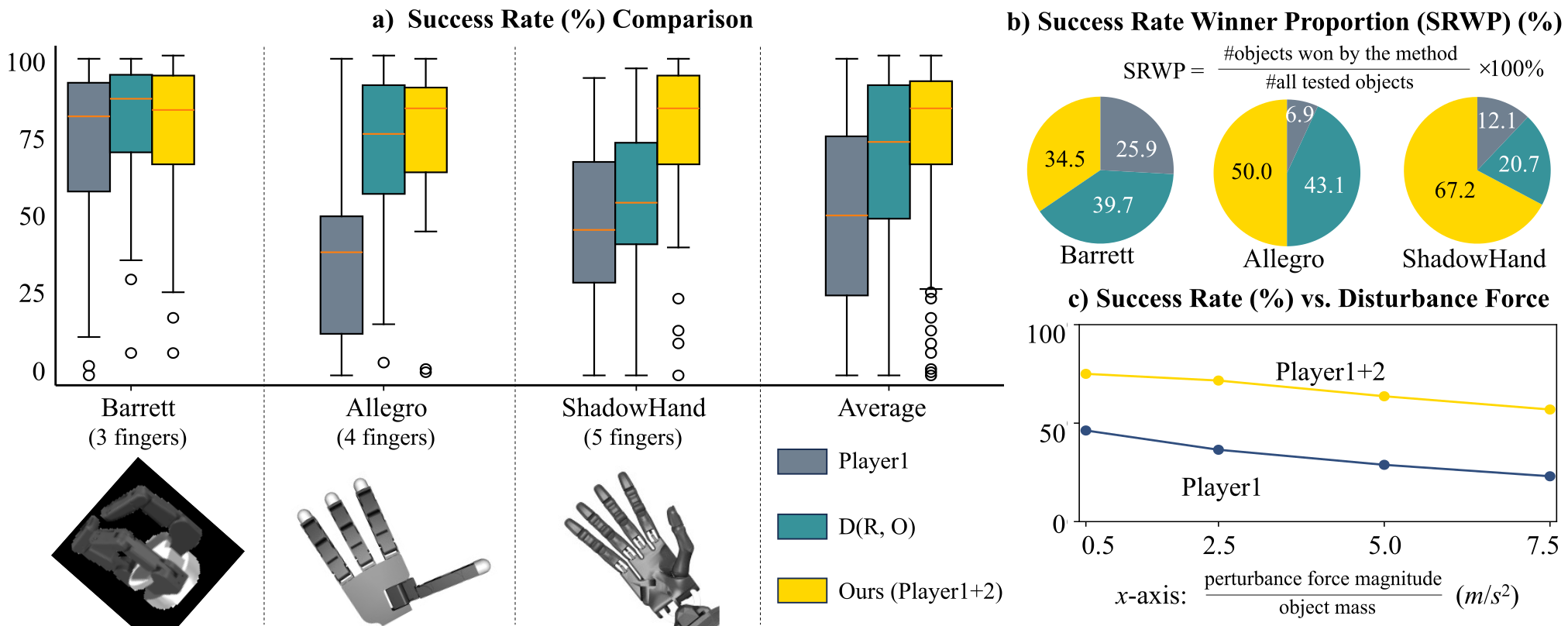
Success is 76.59% on Barrett, 75.74% on Allegro and 75.02% on ShadowHand. D(R,O) is better on Barrett (78.93%); Game4Grasp gains 5.27 points on Allegro and 19.61 on ShadowHand. The three-hand average is 75.78%, 7.51 points above D(R,O).
The detailed results report a 25.56-point average gain over Player1, while the abstract/introduction state 27.40. The original conflicting claims are not silently reconciled. These differences are percentage points, not relative percentages.
The share of objects won is 34.5%/50.0%/67.2% for Game4Grasp on Barrett/Allegro/ShadowHand; D(R,O) wins 39.7% of Barrett objects. Thus the advantage grows with these hand configurations but is not uniform across every hand. Tie handling is unspecified.
On ShadowHand, increasing disturbance acceleration from 0.5 to 7.5 m/s² lowers success, while the adversarial method remains above Player1. This is evidence under the tested forces, not robustness to arbitrary disturbances or sensor errors.
V-A 4 Runtime Analysis
C++ runs on a Core i7 laptop with 16 GB RAM. Detailed mean runtimes are 0.26 s for Barrett, 0.78 s for Allegro and 1.04 s for ShadowHand; the abstract instead starts its range at 0.28 s. Means are not worst-case latency bounds, and the ShadowHand mean slightly exceeds one second.
V-B Extreme-Case Robustness Evaluation: Grasping Cross-Category Deforming Object
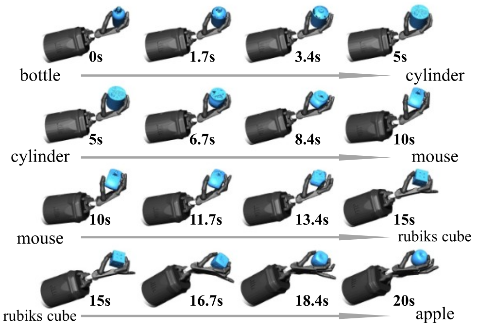
A ShadowHand in MuJoCo holds a mesh that morphs through bottle, cylinder, mouse, Rubik’s cube and apple shapes. Blender creates one hundred intermediate meshes per five-second transition. After the first grasp, each solve starts from the preceding hand pose; optimization runs at 1 Hz and the PID controller at 200 Hz.
The illustrated sequence completes without failure. It is a constructed mesh-transition case without reported repeated-trial statistics or baseline comparison, not a physical deformable-material experiment. It suggests adaptability while leaving cloth, compliant materials and tool-use performance untested.
| Object | tuna can | drill | tomato can | mustard | Avg. |
|---|---|---|---|---|---|
| LeapHand | 8/10 | 9/10 | 10/10 | 8/10 | 87.5 |
| ShadowHand | 9/10 | 8/10 | 7/10 | 10/10 | 85.0 |
V-C Real-Robot Experiments
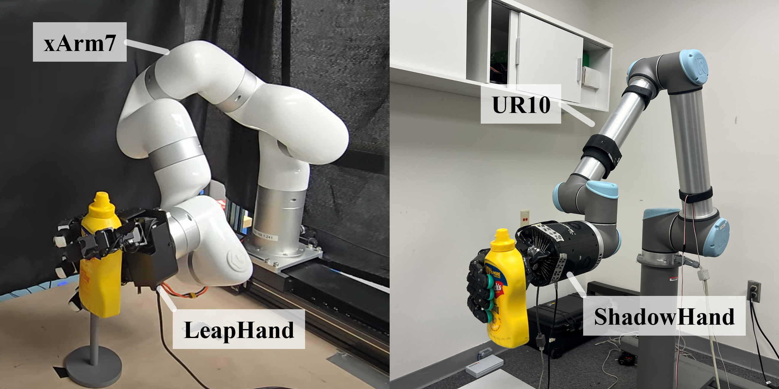
Hardware uses xArm7 with LEAP Hand and UR10 with ShadowHand. Each hand tests a tuna can, drill, tomato can and mustard container ten times each. Success requires holding the object for three seconds.
LEAP Hand succeeds on 35/40 trials (87.5%) and ShadowHand on 34/40 (85%). No hardware baseline or matched six-direction disturbance test is reported, so these figures demonstrate static holding feasibility rather than the same robustness metric used in simulation.
VI Conclusions and Future Work
The two-player search improves the tested geometric grasps, especially for the four- and five-finger hands. Its useful contribution is incorporating candidate escape motions during synthesis, with practical local optimization and explicit feasibility constraints.
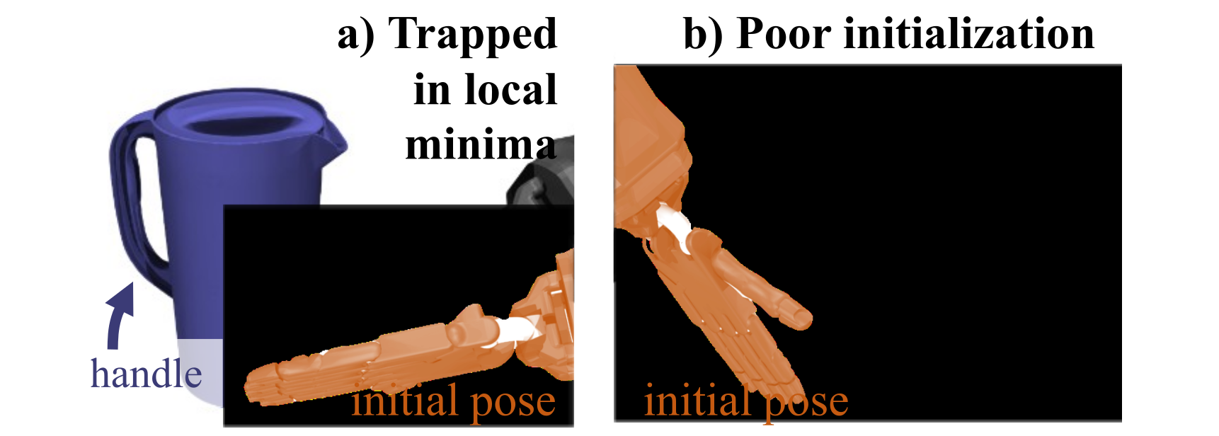
The friction-free condition can be overly conservative or infeasible for large or symmetric objects. Local minima can trap a hand away from a useful handle, and PCA initialization can fail on complex shapes such as the illustrated airplane. Friction-aware modeling, stronger game solvers and better initialization remain future work.