Overview
This edition follows the 49-page arXiv version 1, dated 6 November 2025. It retains all 25 numbered figures, 17 numbered tables, four algorithms, and the full bibliography, including the appendix’s benchmark examples and training details. The paper separates a spatially trained video model from an additional prediction-guided memory prototype.



At a glance
Cambrian-S combines a curated spatial question-answer dataset with a four-stage multimodal training pipeline. It reaches 67.5 on VSI-Bench but struggles with long streams. The authors introduce VSI-Super recall and counting tasks, then add next-frame latent prediction to guide memory compression and event segmentation. The resulting improvements support a useful prototype for structured long-video processing; they do not demonstrate human-level spatial cognition or a general predictive world model.
1 Introduction
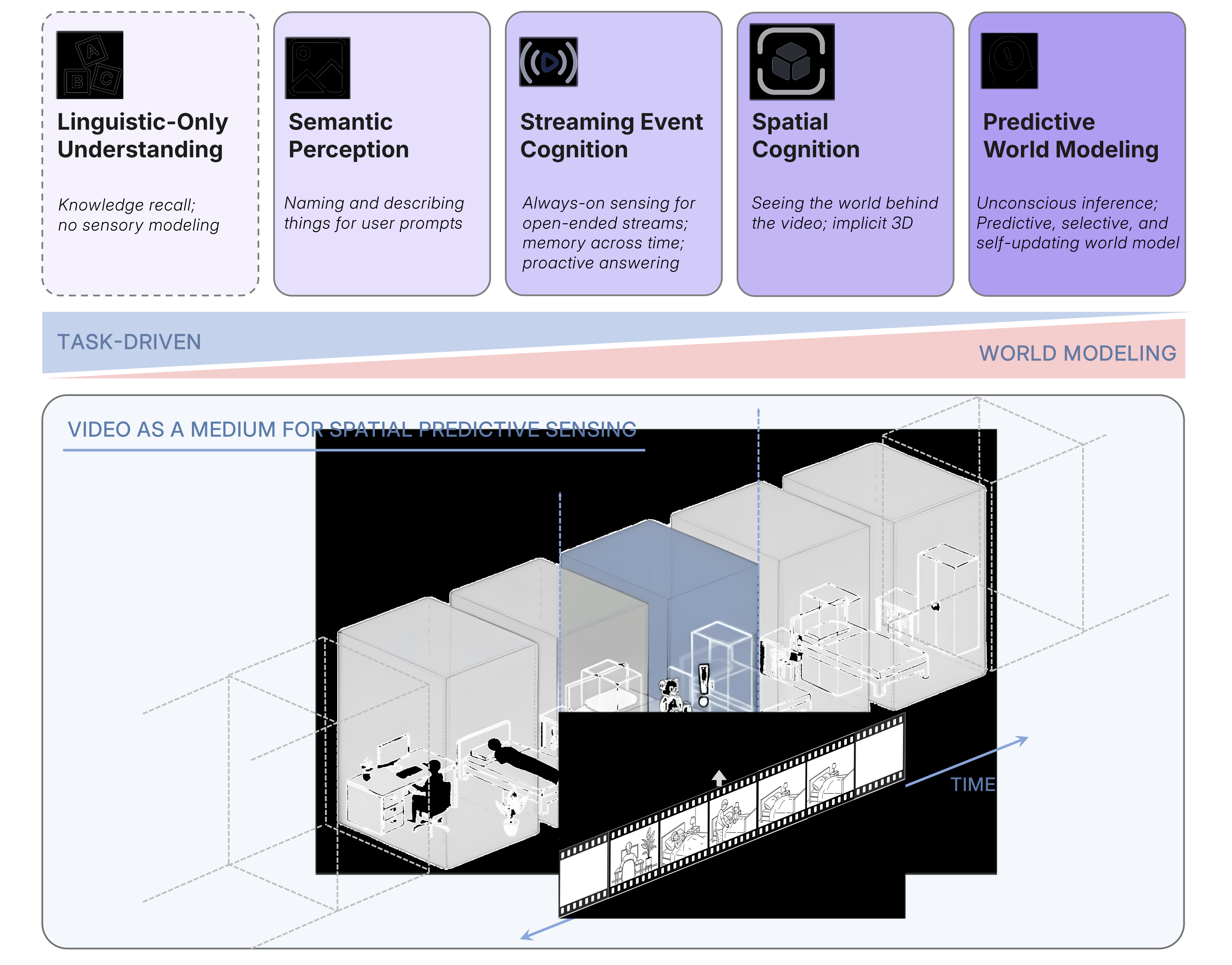
The proposed hierarchy progresses from semantic perception through continuous-event memory and implicit 3D cognition to predictive world modeling. This is a conceptual research agenda, not a measured developmental law. Three contributions test parts of it: diagnosing existing benchmarks, constructing spatial training data and Cambrian-S, and using prediction error to select and organize memories. The paper explicitly does not claim to realize the complete “supersensing” goal.
2 Benchmarking Spatial Supersensing
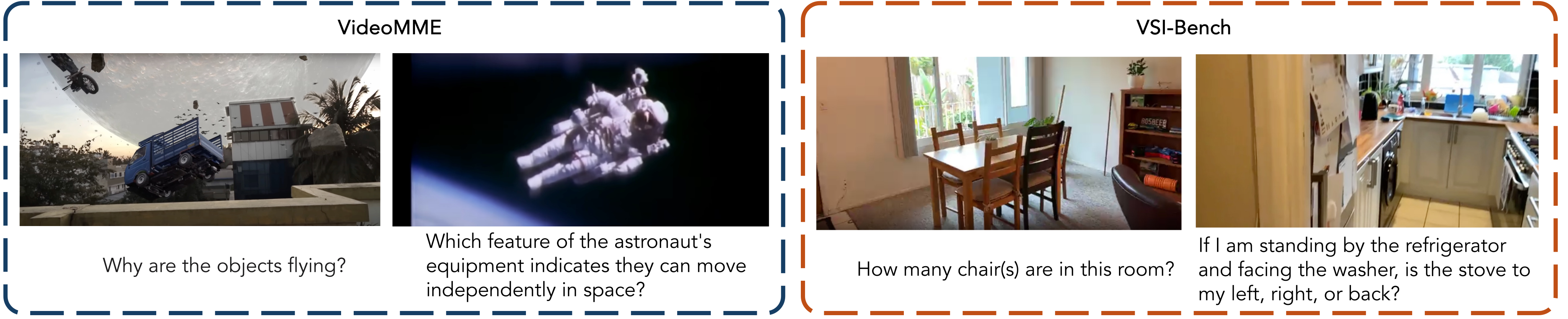
Benchmarking first asks what existing video questions actually require, then introduces long-duration spatial recall and counting tasks. Different benchmarks measure different abilities, so their scores are not interchangeable measures of video understanding.
2.1 Deconstructing Existing Video Benchmarks
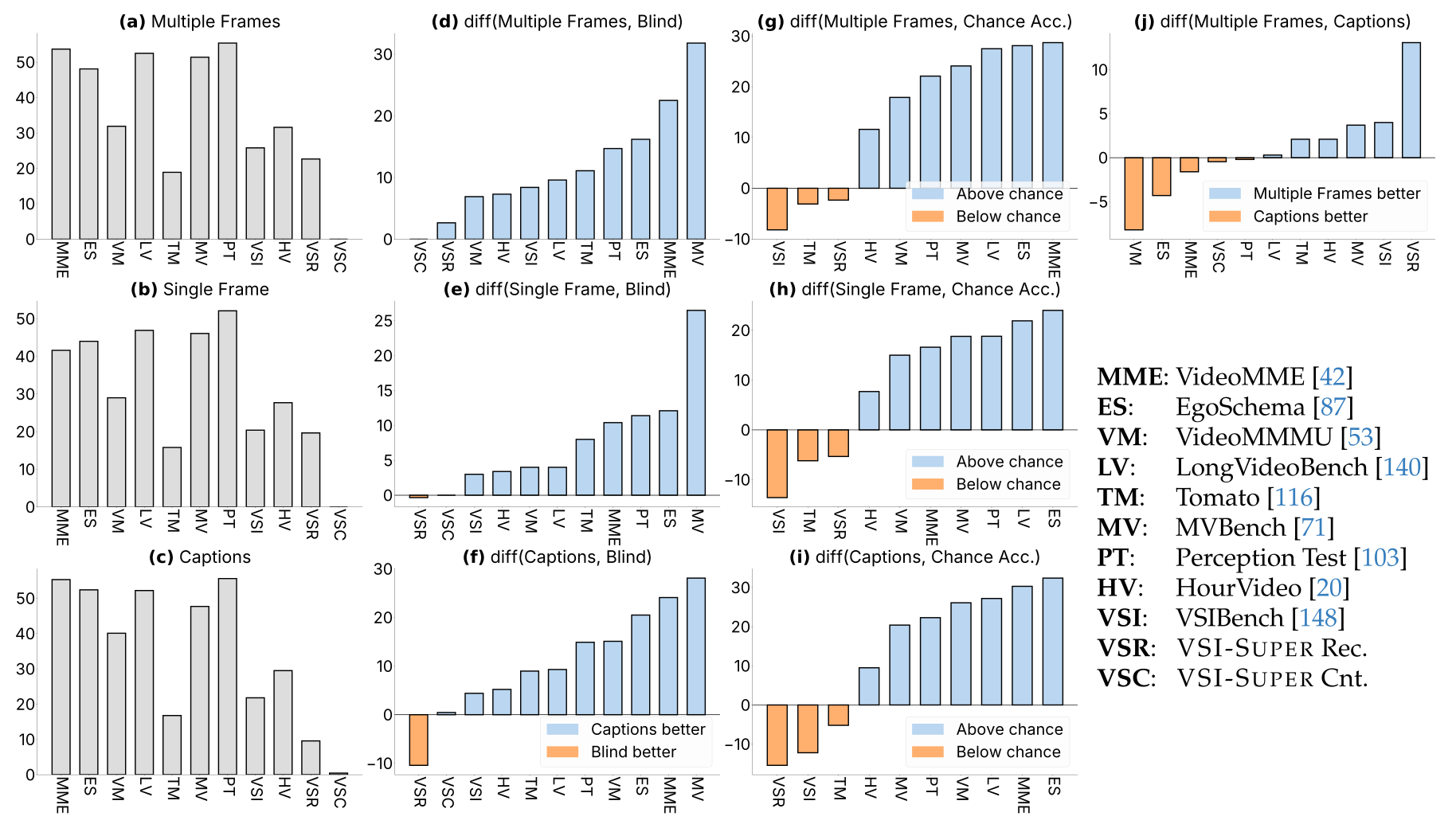
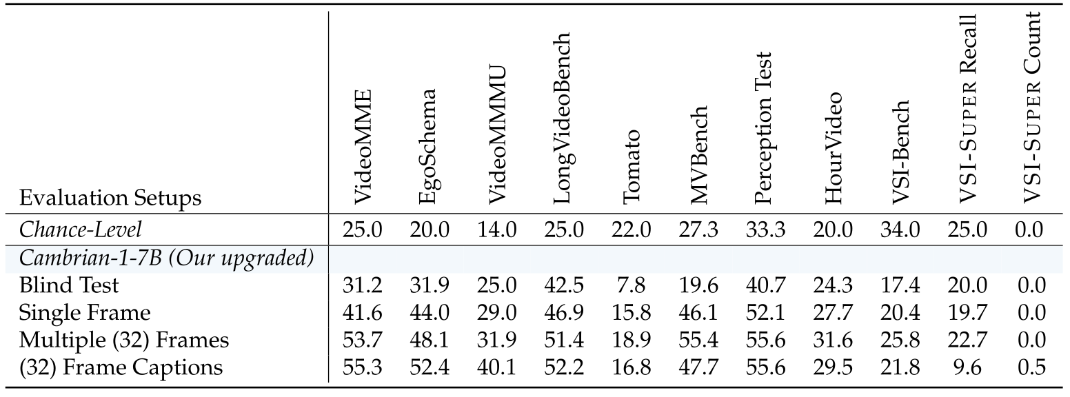
An upgraded image-only Cambrian-1 receives 32 sampled frames, one middle frame, captions of those frames, or no visual information. Captions generated by Gemini-2.0-Flash often match or outperform direct frames on semantic benchmarks; VSI-Bench and Tomato are harder. Caption inputs still contain visual evidence translated by another model, so this is not a pure language-prior control. Results depend on the chosen model, captioner, and temporal sampling, and do not establish that a benchmark universally needs no vision. Near-zero VSC scores prevent meaningful comparisons among these input modes.
2.2 VSI-Super : Towards Benchmarking Spatial Supersensing in Multimodal LLMs
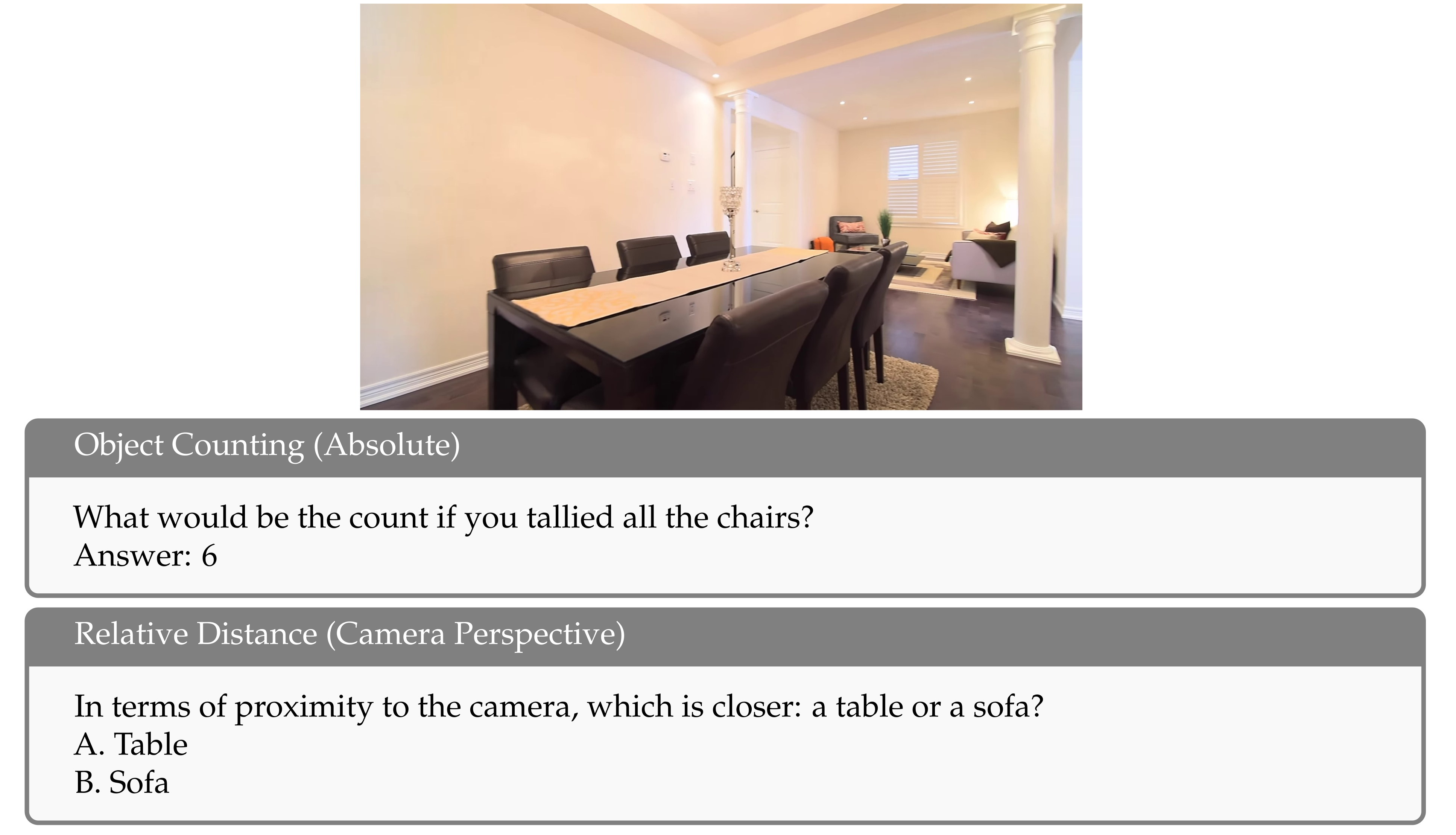
VSI-Super tests ordered recall of unusual objects and cumulative counting across concatenated room tours. Its variable durations deliberately stress fixed context windows. These synthetic constructions expose practical memory weaknesses, while their relevance to natural continuous experience remains an empirical question.
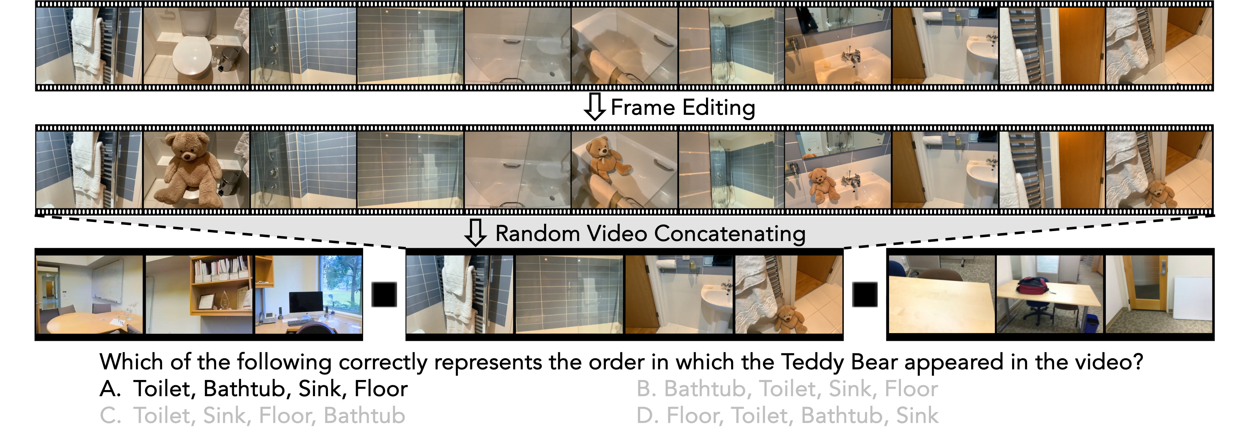
VSI-Super Recall: Long-horizon spatial observation and recall.
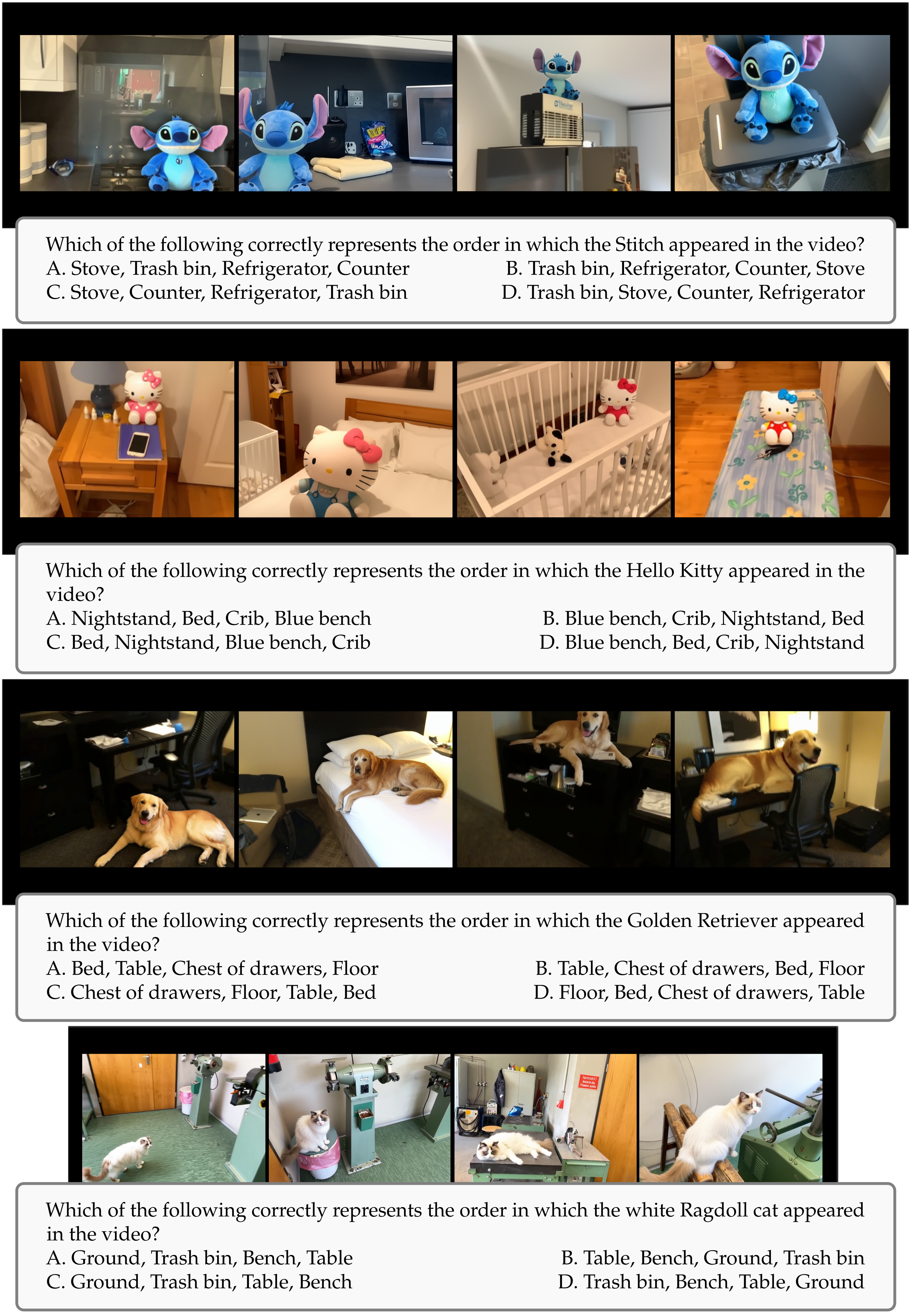
For VSR, annotators insert the same unusual object into four distinct frames and locations, then concatenate the edited room tour with other tours. A multiple-choice question asks for the locations in appearance order. Five durations run from ten minutes to four hours. This is spatially contextualized needle recall, with temporally sparse edited events rather than naturally persistent objects.
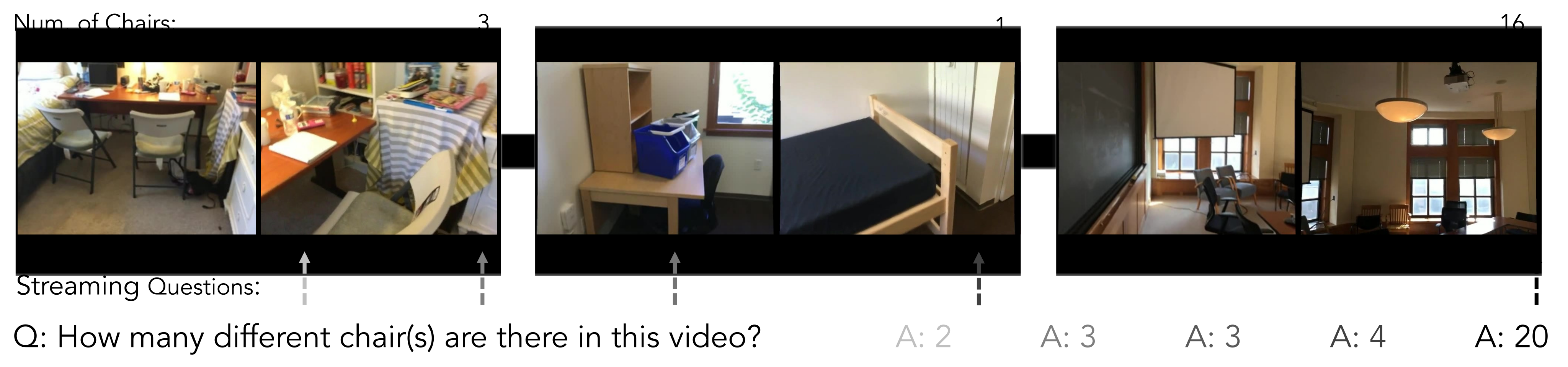
VSI-Super Count: Continual counting under changing viewpoints and scenes.
VSC concatenates tours and asks for the total number of a target object category across rooms, with durations of 10, 30, 60, and 120 minutes. Viewpoint changes and repeated sightings within a tour require avoiding duplicate counts. Evaluation uses the inherited mean relative accuracy metric, which should not be read as the percentage of exactly correct counts. Streaming evaluation repeats the question at intermediate times.
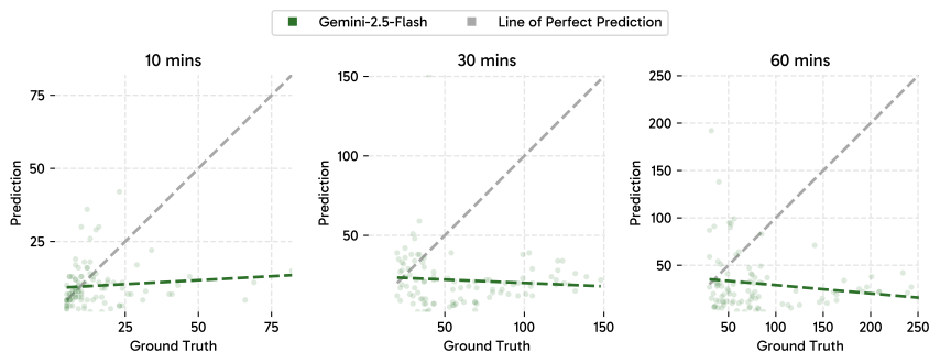
State-of-the-art models struggle on VSI-Super .
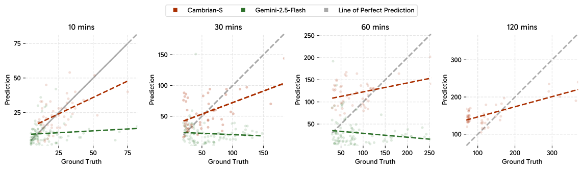
Gemini-2.5-Flash scores 81.5/79.2 on VideoMME/VideoMMMU but 41.5 on one-hour VSR and 10.9 on one-hour VSC. Two-hour inputs exceed its tested context budget. Its counts saturate at small values as true counts grow, consistent with poor extrapolation under this setup; the plots do not independently identify reliance on training priors as the cause.

How VSI-Super challenges the current paradigm.
An arbitrarily extensible stream cannot be retained verbatim in a fixed window. The authors therefore motivate selective memory and decomposition into local events. The experiments show limitations of the tested sampling and memory strategies, rather than proving that every possible data-scaled multimodal architecture must fail or that prediction error is the only solution.
3 Spatial Sensing Under the Current Paradigm
The data-driven baseline first strengthens image understanding, then general video understanding, then spatial skills. This provides a strong short-video model before testing whether a separate memory mechanism improves longer streams.
3.1 Base Model Training: Upgraded Cambrian-1
The base replaces Cambrian-1’s visual encoder with SigLIP2-So400M, uses instruction-tuned Qwen2.5, and connects them with a two-layer MLP. The simpler connector trades the earlier deep visual fusion for computational efficiency.
3.2 Spatial Video Data Curation: VSI-590K
VSI-590K targets spatial relationships absent from much general instruction data. It mixes geometry-derived video questions, simulated scenes, and pseudo-annotated real images; those sources have different supervision quality and modalities.
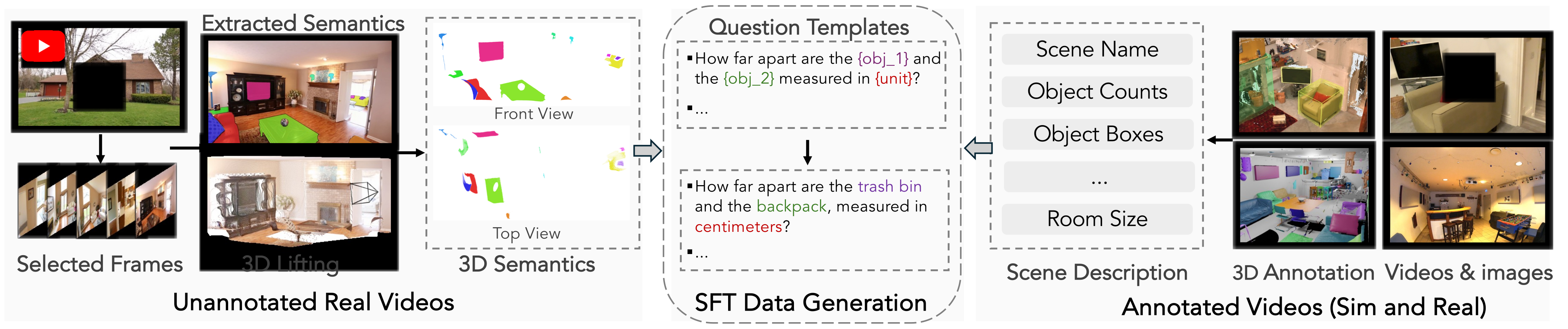
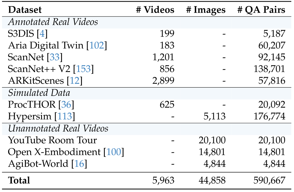
Data curation and processing.
The final dataset contains 590,667 question-answer pairs from 5,963 videos and 44,858 images across ten sources. Annotated indoor scans and egocentric videos supply instance geometry. ProcTHOR contributes 625 simulated traversals, and Hypersim contributes 5,113 images. Around 19K web room tours and robot datasets supply frames processed with detection, segmentation, and reconstruction. Pseudo-labeling is performed per image because full-video reconstruction is noisier.
Question type definition and template augmentation.
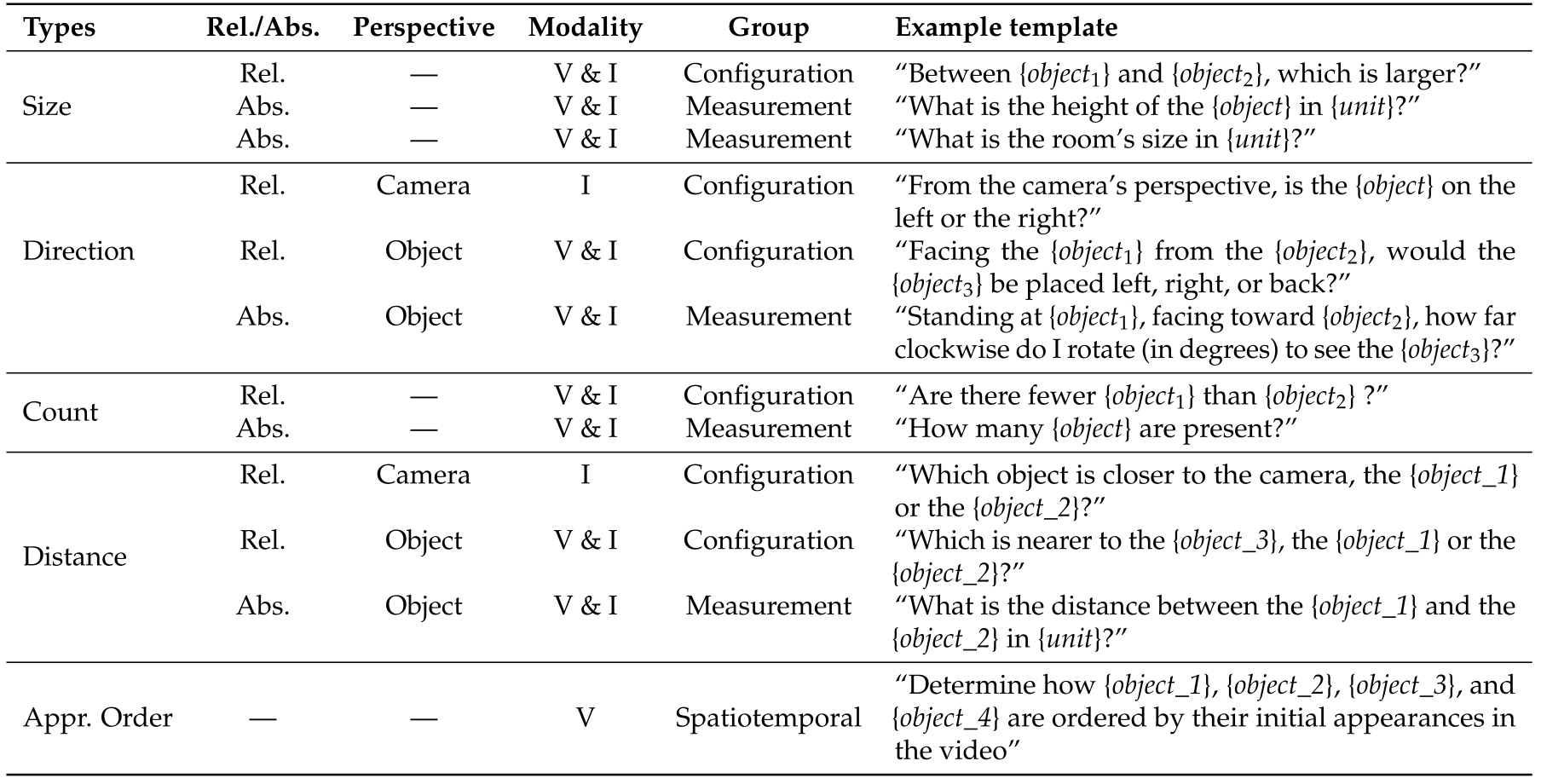
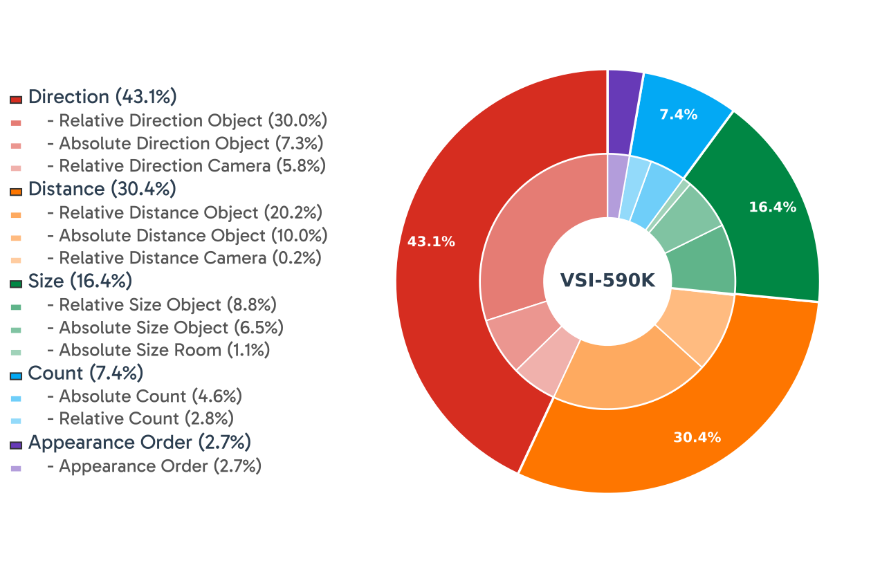
Twelve question types cover size, direction, count, distance, and appearance order, with relative/absolute distinctions and camera/object viewpoints. Templates vary wording and measurement units. The resulting mixture emphasizes configuration questions; appearance order requires video and forms a small portion of the corpus.
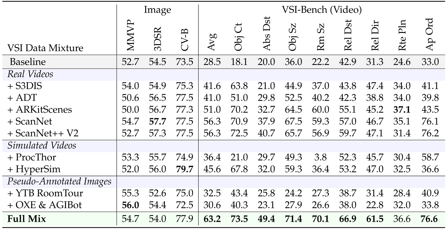
VSI-590K data source ablation.
The full source mixture reaches 63.2 on the VSI-Bench ablation, versus 28.5 for its baseline. Annotated real videos help most among individual sources, followed by simulated data and pseudo-annotated images. This supports the particular data mixture. Since annotation quality, content, quantity, and modality differ together, it does not isolate an inherent superiority of all video data over all image data.
3.3 Post-Training Recipe for Spatial Sensing
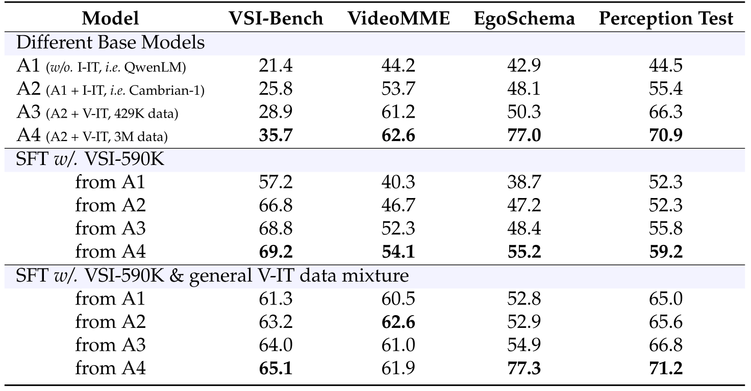
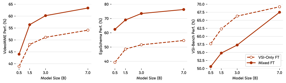
Four initializations progress from alignment-only to image instruction tuning, then 429K or 3M video examples. Stronger video initialization improves subsequent spatial tuning. From the strongest base, spatial-only tuning gives 69.2 VSI-Bench but 54.1 VideoMME; mixed tuning gives 65.1 and 61.9. Thus general-video examples mitigate a real specialization tradeoff rather than preserving every capability automatically.
3.4 Cambrian- S : Spatially-Grounded MLLMs
Cambrian-S uses Qwen2.5 backbones of 0.5B, 1.5B, 3B, and 7B parameters. Alignment and image instruction tuning precede general video tuning on CambrianS-3M. The final stage mixes VSI-590K with general video and image data. These model scales describe the language backbones, with a visual encoder and connector added.

3.5 Empirical Results: Improved Spatial Cognition
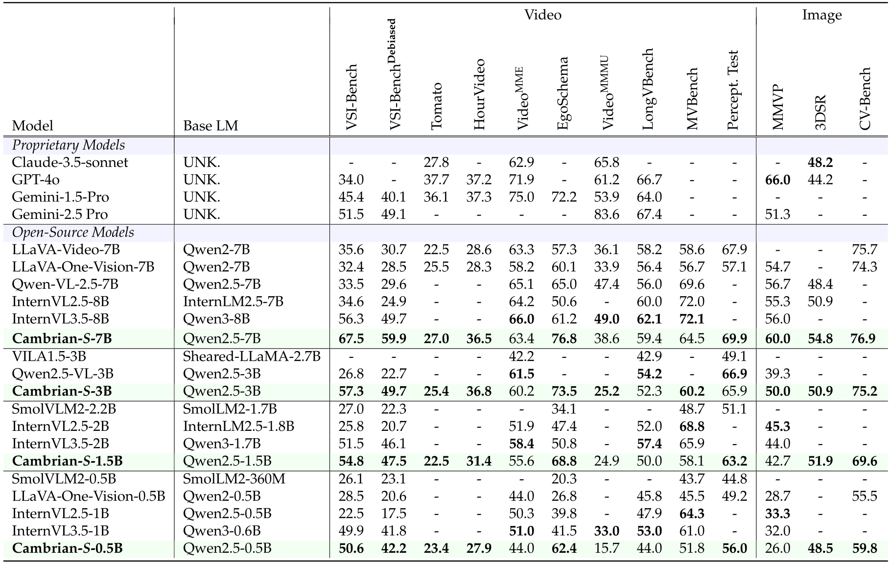
Evaluation reports standard spatial tests, debiased tests, general benchmarks, and long-video failures. Good short-video spatial scores coexist with weak continual counting and recall.
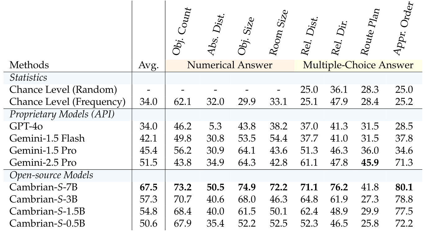
Improved spatial cognition.
The 7B model reaches 67.5 on VSI-Bench, versus Gemini-2.5-Pro’s 51.5 and its own stage-3 score of 35.7. Route planning reaches 41.8 despite that question type being absent from the curated training set; it exceeds Gemini-1.5-Pro’s 36.0 but remains below Gemini-2.5-Pro’s 45.9. The authors report disjoint training versus benchmark splits even when dataset sources overlap. These results support transfer to a held-out task type, not unrestricted spatial generalization.
Robust spatial reasoning on VSI-Bench-Debiased.
VSI-Bench-Debiased reduces opportunities to answer from familiar object-size priors. Cambrian-S-7B falls from 67.5 to 59.9 but remains above Gemini-2.5-Pro’s 49.1. This is additional evidence of visual grounding under the tested debiasing scheme, rather than proof that language shortcuts are entirely absent.
Results on VSI-Super: limitations in continual spatial sensing.
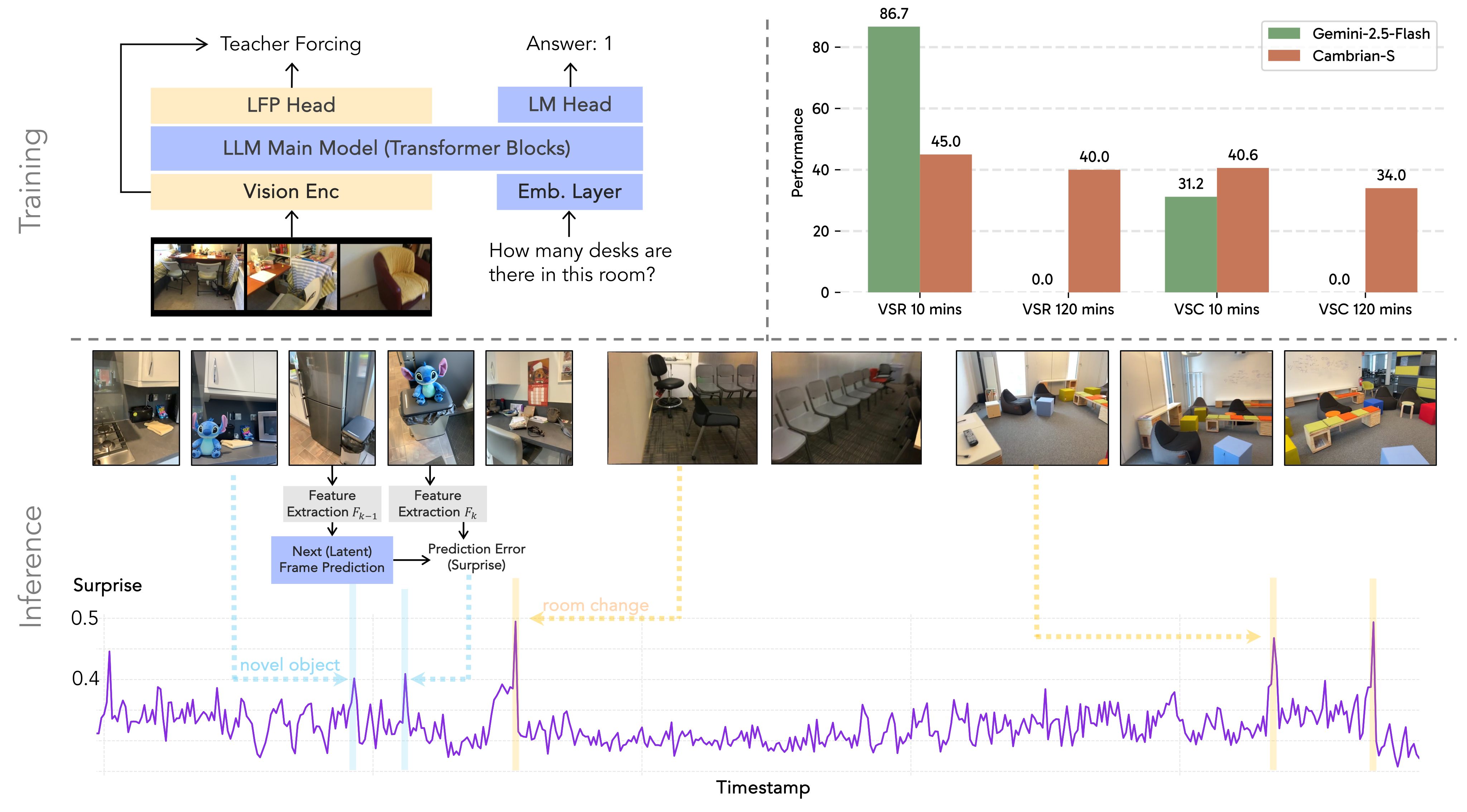
With one-frame-per-second streaming input, base Cambrian-S-7B VSR scores drop from 38.3 at ten minutes to 35.0 at thirty and 6.0 at sixty, then zero at longer durations. VSC is 0.6 at ten minutes and zero thereafter. Uniformly sampling 128 frames from an entire completed video is reported separately because it uses an offline view of the stream and can miss sparse events. These failures motivate explicit memory mechanisms.

4 Predictive Sensing as a New Paradigm
Predictive sensing adds a lightweight latent-frame prediction objective, then uses prediction error as a control signal. The demonstrated functions are memory allocation and boundary detection. Predicting visual features does not by itself establish a coherent 3D world model, causal dynamics, or action-conditioned planning ability.
4.1 Predictive Sensing via Latent Frame Prediction
A two-layer MLP predicts the next frame’s visual representation from the language model’s contextual state. Training adds mean-squared and cosine losses to instruction tuning, using a 290K video subset sampled at 1 FPS for the prediction objective. The connector, language model, and both heads are jointly updated; SigLIP remains frozen. Later experiments still call this modified checkpoint Cambrian-S, so it should be distinguished from the earlier spatial-only model.
Inference: Estimating surprise via prediction error.
At inference, cosine distance between the predicted next-frame feature and the observed feature supplies a surprise score. High error can signal an unusual object or a scene transition, but can also arise from motion, nuisance changes, or model error; it is a learned feature discrepancy rather than calibrated semantic novelty.
4.2 Case Study I: Surprise-driven Memory Management System for VSI-Super Recall.
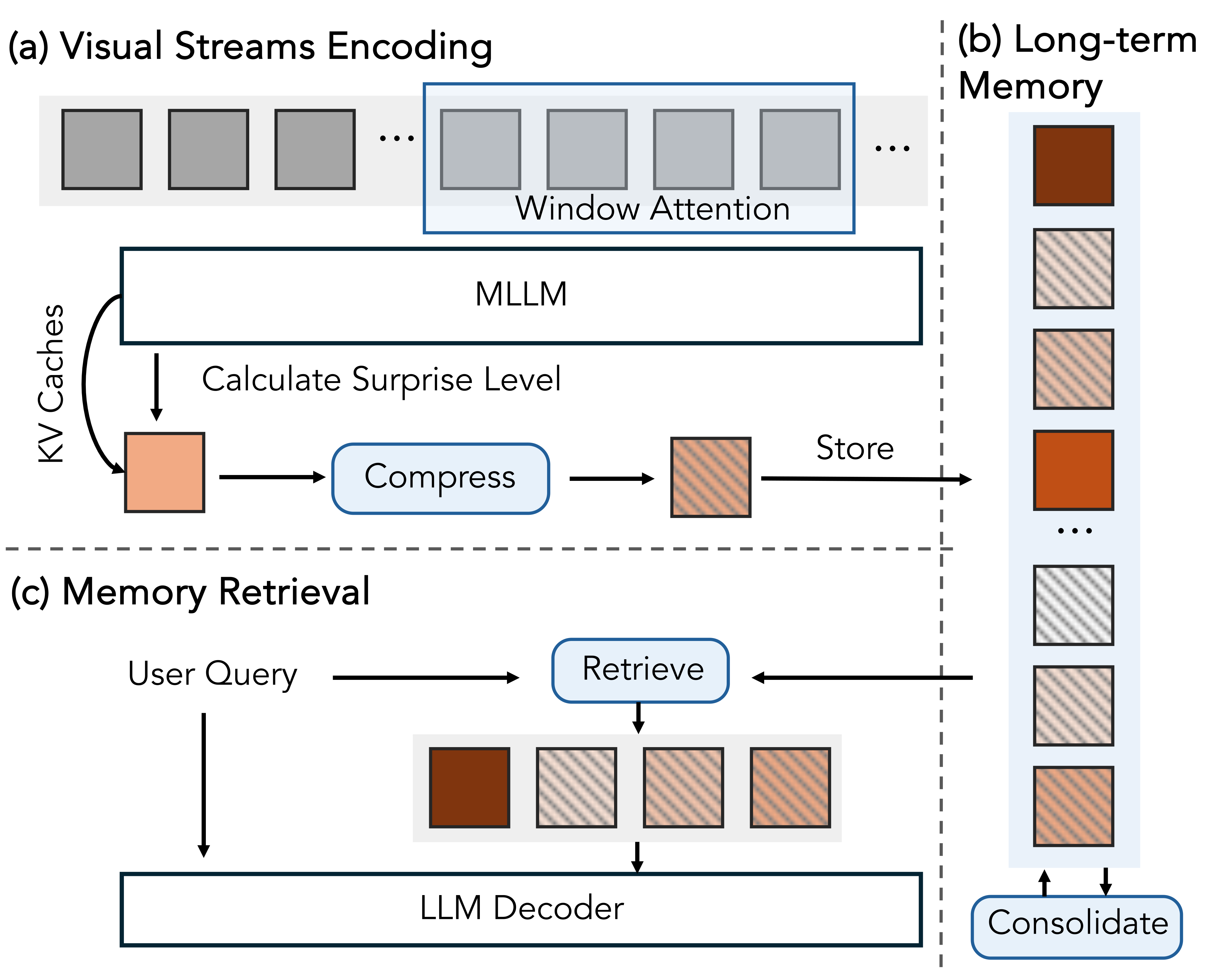
The recall prototype keeps a bounded long-term store and retrieves relevant memories only when a query arrives. Surprise guides retention before the future question is known.
Surprise-driven memory management system.
Incoming frames are encoded with a fixed sliding context window. Low-surprise frame key/value caches undergo spatial downsampling before entering long-term memory. When the token budget is exceeded, consolidation drops or merges memories using surprise. A query then selects top-K relevant frames through query–key feature similarity. This bounds the stored representation, while total processing work still grows with stream duration.
Results.
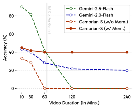
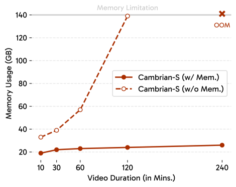
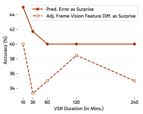
The memory variant scores 45.0, 41.7, 40.0, 40.0, and 40.0 on VSR from ten minutes to four hours. It is stable but far from perfect recall. Gemini-2.5-Flash is much stronger at ten minutes, with 86.7, and remains competitive within its supported context; the proposed method’s clearest advantage is sustaining processing beyond that limit. Memory usage remains roughly 20–25 GB over the plotted durations, unlike the growing uncompressed baseline. Figure 11 labels its secondary baseline Gemini-2.0-Flash, while the accompanying prose calls it Gemini-1.5-Flash; that source discrepancy is retained.
Ablation on surprise measurement.
Prediction-error surprise outperforms adjacent-frame SigLIP feature difference under the same memory design. Thresholds are tuned separately for both methods at each duration. The paper does not detail an independent threshold-validation split, so this is a tuned comparison rather than evidence that one fixed threshold generalizes to arbitrary streams.
4.3 Case Study II: Surprise-driven continual video segment for VSI-Super Count.
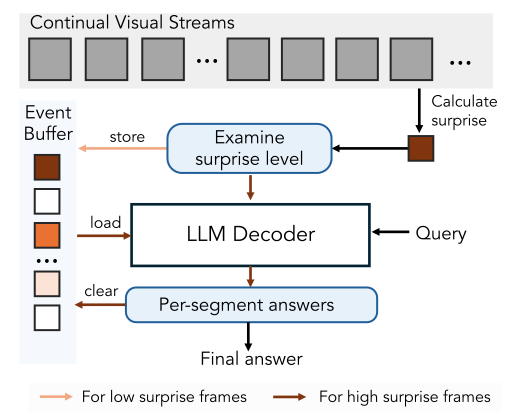
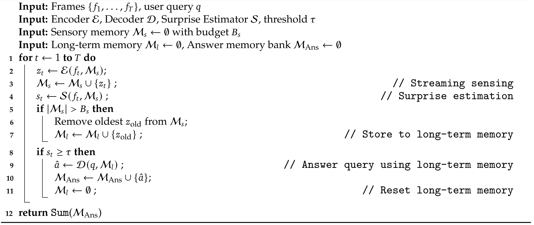
The counting prototype divides the video into local events, answers the counting query for each segment, and sums the intermediate answers. Its benefit comes from both segmentation and explicit numerical aggregation.
Surprise-driven event segmentation.
A large surprise score triggers decoding from the accumulated event memory and resets that memory. This approximately aligns segments with room-tour transitions. The method assumes that summing segment counts is meaningful; revisiting the same physical objects across arbitrary event boundaries would need additional identity handling not demonstrated by concatenated tours.
Results.
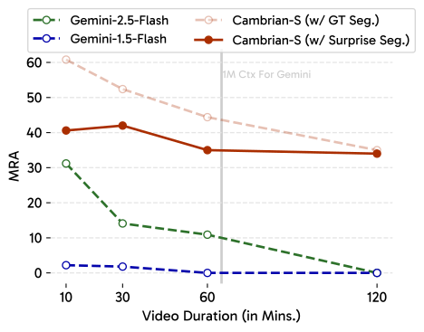
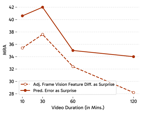
Surprise segmentation yields VSC MRA of 40.6, 42.0, 35.0, and 34.0 over 10–120 minutes. Ground-truth boundaries improve results further, suggesting imperfect segmentation remains a bottleneck. Predicted counts scale more closely with true counts than Gemini’s, but scatter and systematic errors remain. These scores do not mean exact counting on 34–42% of samples.
Ablation on surprise measurement.
Using prediction error for boundaries beats adjacent-frame similarity at all tested durations after tuning both methods. This isolates the signal within the implemented pipeline more directly than comparisons against whole commercial systems, but does not show that all simpler or task-specific segmentation methods are inferior.
Evaluation in streaming setup.
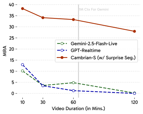
Streaming evaluation asks the same cumulative-count question at ten timestamps and averages the scores. Cambrian-S obtains about 38 MRA at ten minutes and 28 at two hours; tested Gemini-Live and GPT-Realtime configurations are below 15 at ten minutes and near zero at two hours. This is a benchmark-specific live-input comparison, not an overall assessment of conversational assistants or deployment latency.
Summary.
Both case studies support selective storage and structured accumulation for these long-video tasks. Claims about unbounded human-level or superhuman spatial intelligence remain the paper’s motivating direction, beyond its measured evidence.
5 Related Work
Related work spans multimodal language models, long-stream processing, spatial intelligence, and predictive representations.
Video Multimodal Large Language Models
Video models typically combine pretrained visual representations with language models and instruction tuning. Cambrian-S studies how their data, evaluation, and objectives can be adapted for spatial tasks rather than introducing a wholly independent perception system.
Streaming Video Understanding
Existing approaches use efficient attention, larger context windows, retrieval, and token compression. The proposed contribution is prediction-error-guided memory organization, situated alongside these engineering methods rather than a proof that sequence modeling cannot support continual perception.
Visual Spatial Intelligence
Spatial benchmarks and training methods study object relations, geometry, viewpoint changes, and embodied grounding. VSI-590K and VSI-Super emphasize video-based spatial reasoning and long-duration information retention.
Predictive Modeling
Predictive coding, self-supervised representations, learned world models, and model predictive control motivate anticipating observations. The current prototype predicts latent visual features; it does not implement the control or multi-step simulation capabilities of those broader approaches.
6 Conclusion
The strongest demonstrated outcomes are improved standard spatial benchmark scores and better sustained recall/counting with prediction-guided memory. The authors acknowledge limitations in benchmark diversity, data quality and scale, generalizability, and model design. Synthetic edits, concatenated rooms, small per-duration test sets, tuned thresholds, and incomplete reproduction details constrain broader conclusions; no human-level evaluation or embodied deployment is shown.
Acknowledgments
The work builds on Cambrian-1, uses Google TPU Research Cloud and cloud credits, and acknowledges infrastructure collaborators, manuscript reviewers, fellowships, and research grants.
Appendix
The appendix provides diagnostic results, benchmark construction, data taxonomy, all training stages, detailed model evaluations, and the predictive-memory algorithms. Its complete example figures are retained alongside the edited explanation.
Appendix A Benchmark Diagnostic Test Results
Table 8 reports the input-ablation diagnostics. For example, VideoMME scores 31.2 blind, 53.7 with 32 frames, and 55.3 with frame captions; VSI-Bench scores 17.4, 25.8, and 21.8 respectively. VSR remains below its 25% chance baseline in these image-model tests, and VSC is essentially zero. This cautions against reading differences near the floor as reliable capability rankings.
Appendix B VSI-Super Benchmark
VSI-Super supplies two distinct tasks and duration suites. The construction procedures make the intended challenges reproducible in outline while also defining their synthetic scope.
B.1 VSI-Super Recall
VSR measures ordered spatial recall of an edited object in long concatenated tours.
Implementation details.
Annotators insert unusual objects with Gemini-2.0-Flash into four selected frames and record their locations and order. Each of five durations has 60 videos and one question per video. Videos are downsampled to 1 FPS so the edited frames are guaranteed visible to the evaluated sampling scheme. This alignment favors detection of the deliberately sparse events and differs from arbitrary real-world sampling.
Visualization.
Figure 18 retains all four edited-frame sequences and questions. The objects are visually plausible within each frame, but the figure does not establish temporally consistent insertion across neighboring frames. Sparse appearance is directly relevant to the surprise-based memory mechanism.
B.2 VSI-Super Count
VSC measures accumulated counts over concatenated source environments, with a separate intermediate-query setting.
Implementation Details.
The construction sums annotated scene counts, normalizes object categories across ScanNet, ScanNet++, and ARKitScenes, and rebalances quantities toward a more uniform distribution. Each duration has 50 corresponding questions. Stored VSC videos are 24 FPS, while the proposed sensing prototype typically samples them at 1 FPS; these are different stages of the pipeline.
Streaming setups.
Ground truth at ten query timestamps uses each unique object’s first appearance, following Thinking in Space / VSI-Bench. Thus streaming targets change only as new objects become observable, rather than using the final scene total at every time.
Appendix C VSI-590K Dataset
Dataset documentation distinguishes geometry-backed labels from pseudo-labels and specifies the question taxonomy. Selected examples illustrate the pipeline but are not a comprehensive label-quality audit.
C.1 Details of Question Type Definition
Questions are organized by physical attribute, relative versus absolute measurement, reference viewpoint, and whether an image or video is required.
Taxonomy.
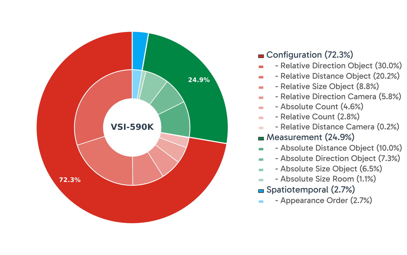
Size, direction, count, distance, and appearance order generate twelve combinations of task type. Configuration accounts for about 72.3% of examples, measurement 24.9%, and spatiotemporal order 2.7%. Relative queries compare objects, absolute queries request quantities, and direction/distance queries vary camera or object reference frames. These are deliberately uneven training proportions.
C.2 Detailed QA-Pair Construction Pipeline
A unified scene representation feeds augmented question templates. Ground-truth geometry and inferred geometry enter that same interface through different collection routes.
3D-annotated real videos.
Real annotated sources provide instance counts, 3D bounding boxes, and room measurements. Their training splits are standardized into scene metadata, then converted to question-answer examples. The approach inherits source annotation accuracy and object-category conventions.
3D-annotated simulated videos and images.
ProcTHOR scenes are traversed from randomized agents, whereas Hypersim supplies annotated individual images. Both use the common template machinery. Simulation supplies controlled geometry but differs from real visual and object distributions.
Unannotated web-crawled real videos.
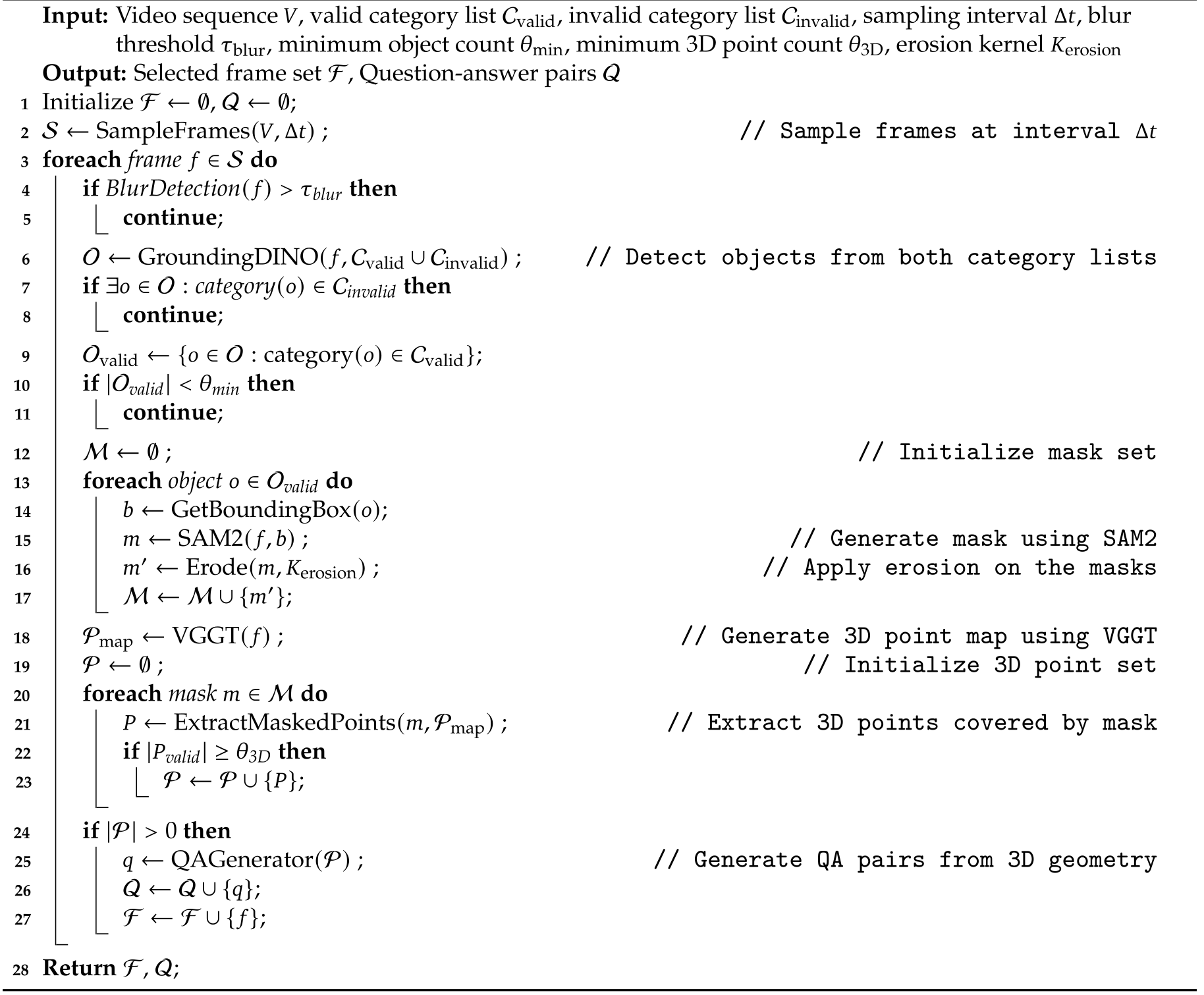
Algorithm 1 samples and filters frames, rejects invalid categories or insufficient objects, runs Grounding DINO and SAM2, erodes masks, and associates them with VGGT point maps. Sufficient valid points then generate questions. Per-frame processing reduces temporal inconsistency but does not eliminate detector, segmentation, scale, or reconstruction errors. All original pseudocode, thresholds-as-symbols, and comments remain visible.
C.3 Additional Ablation Study
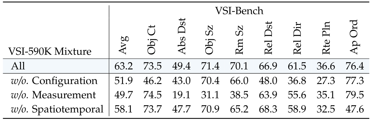
Removing any task group lowers overall VSI-Bench scores from the full mixture’s 63.2. Removing configuration reduces route planning from 36.6 to 27.3; removing measurement gives 35.1, and removing spatiotemporal examples gives 32.5. This supports complementary training groups, without isolating whether differences arise from type, quantity, or difficulty.
C.4 Examples of VSI-590K
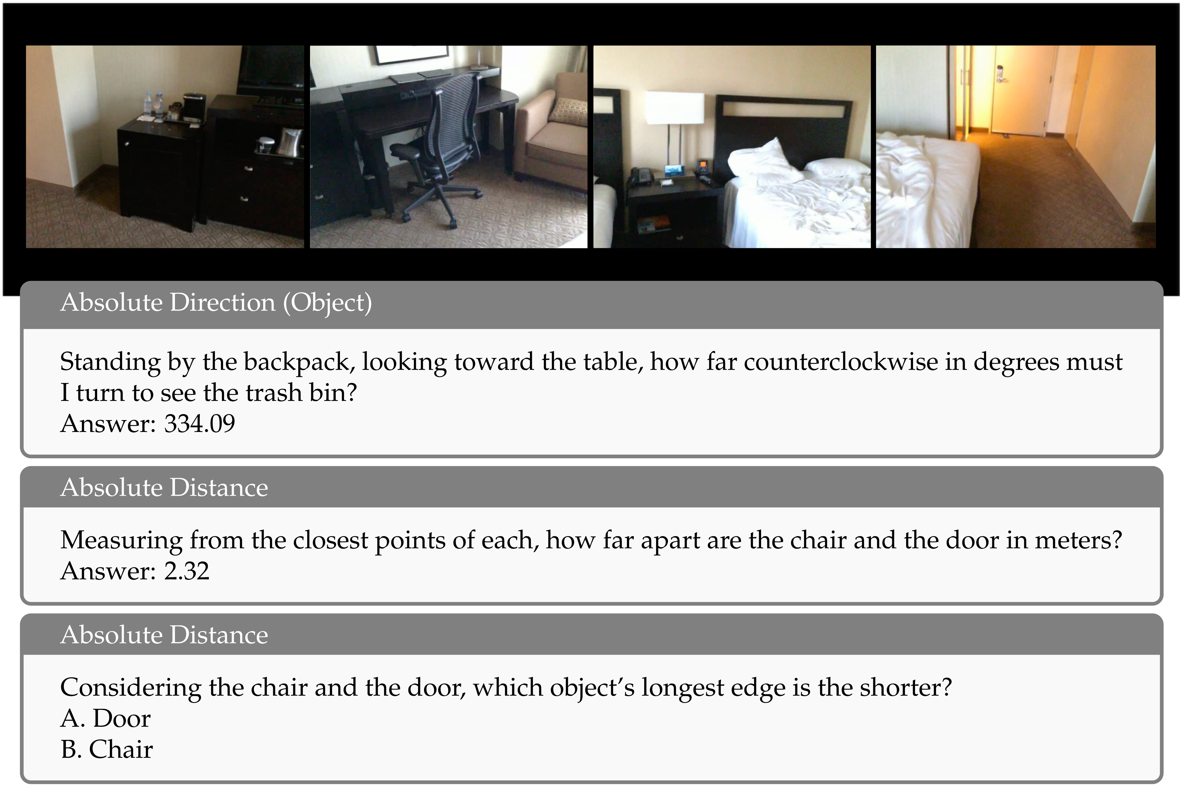
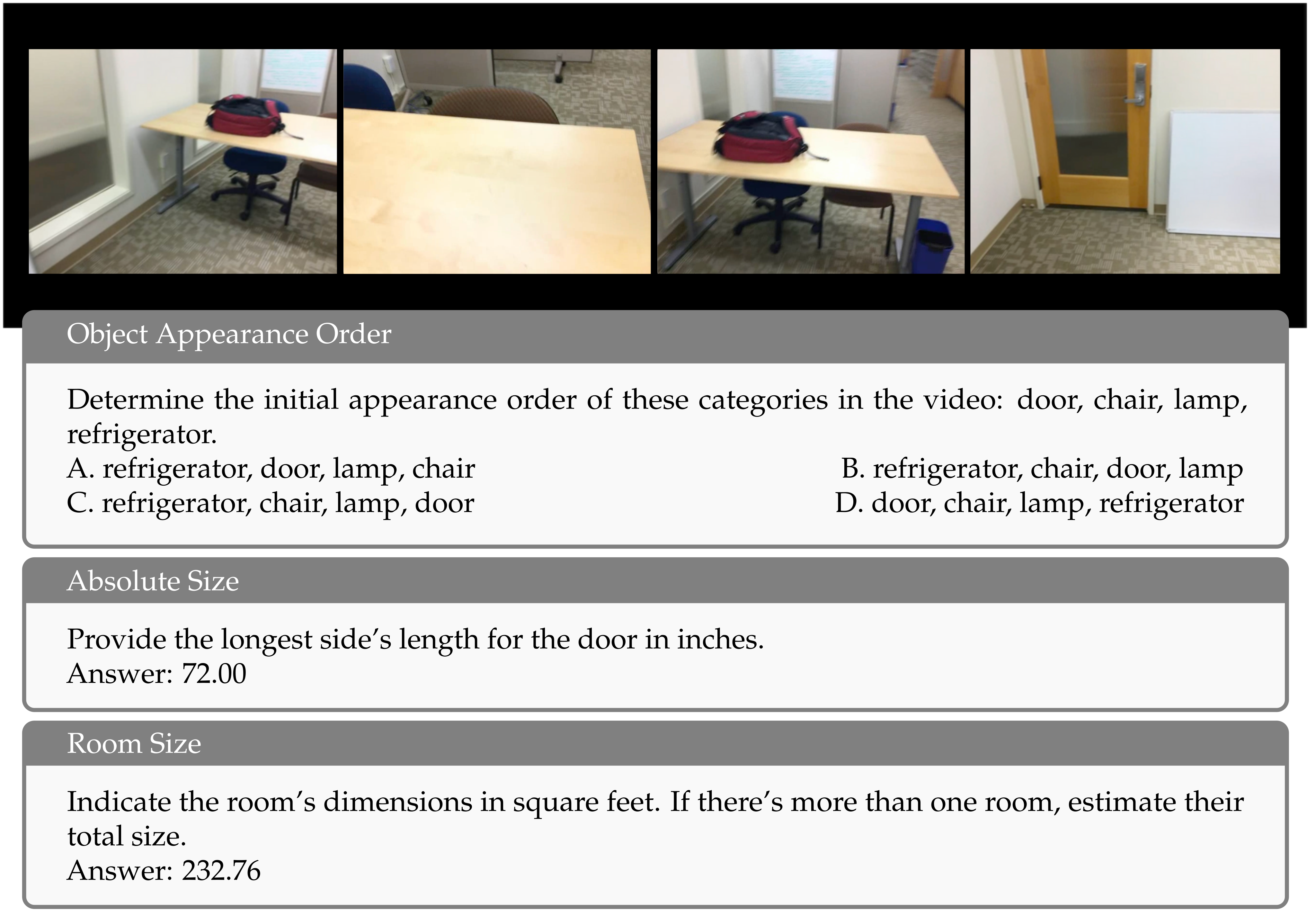
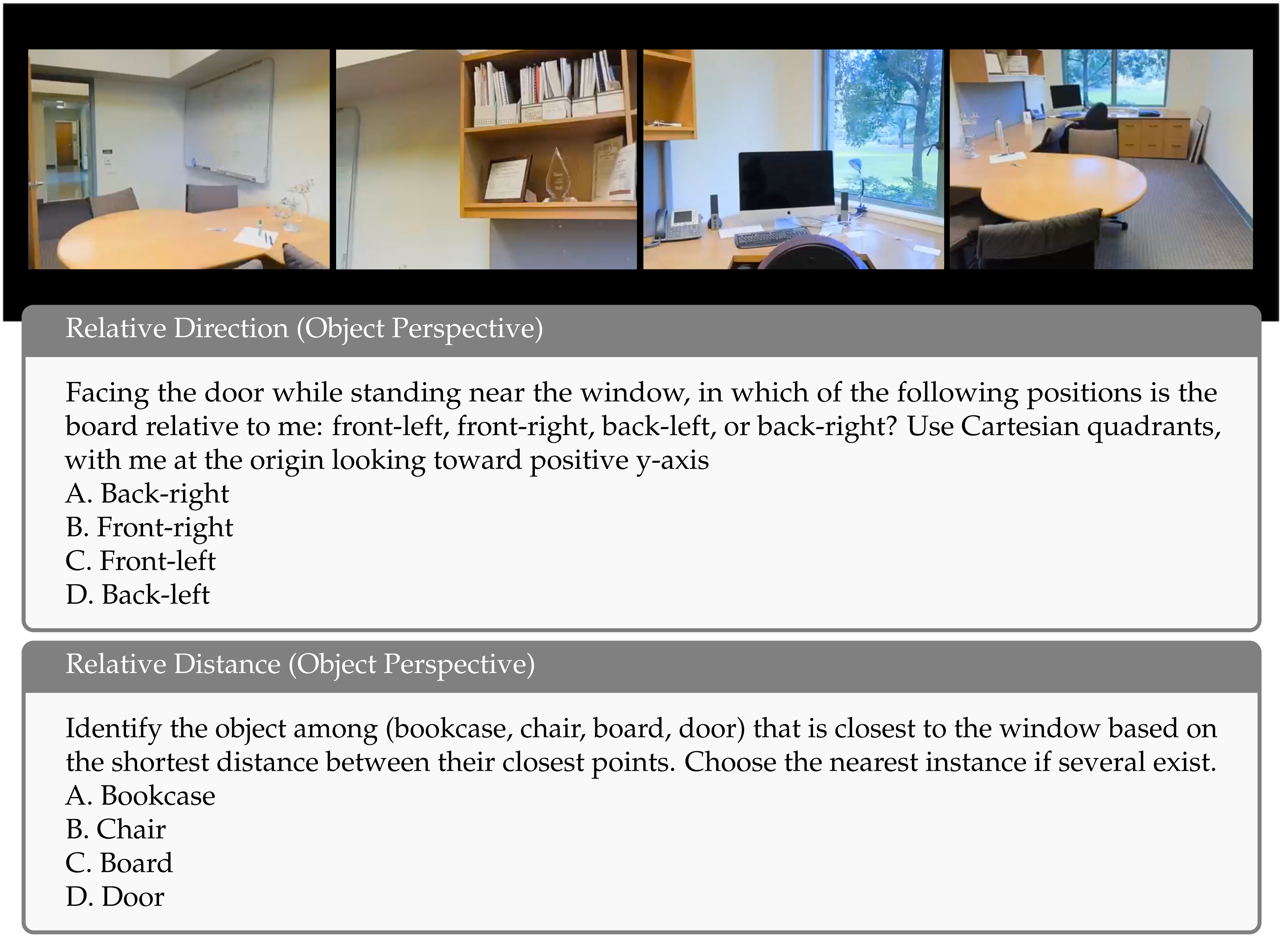
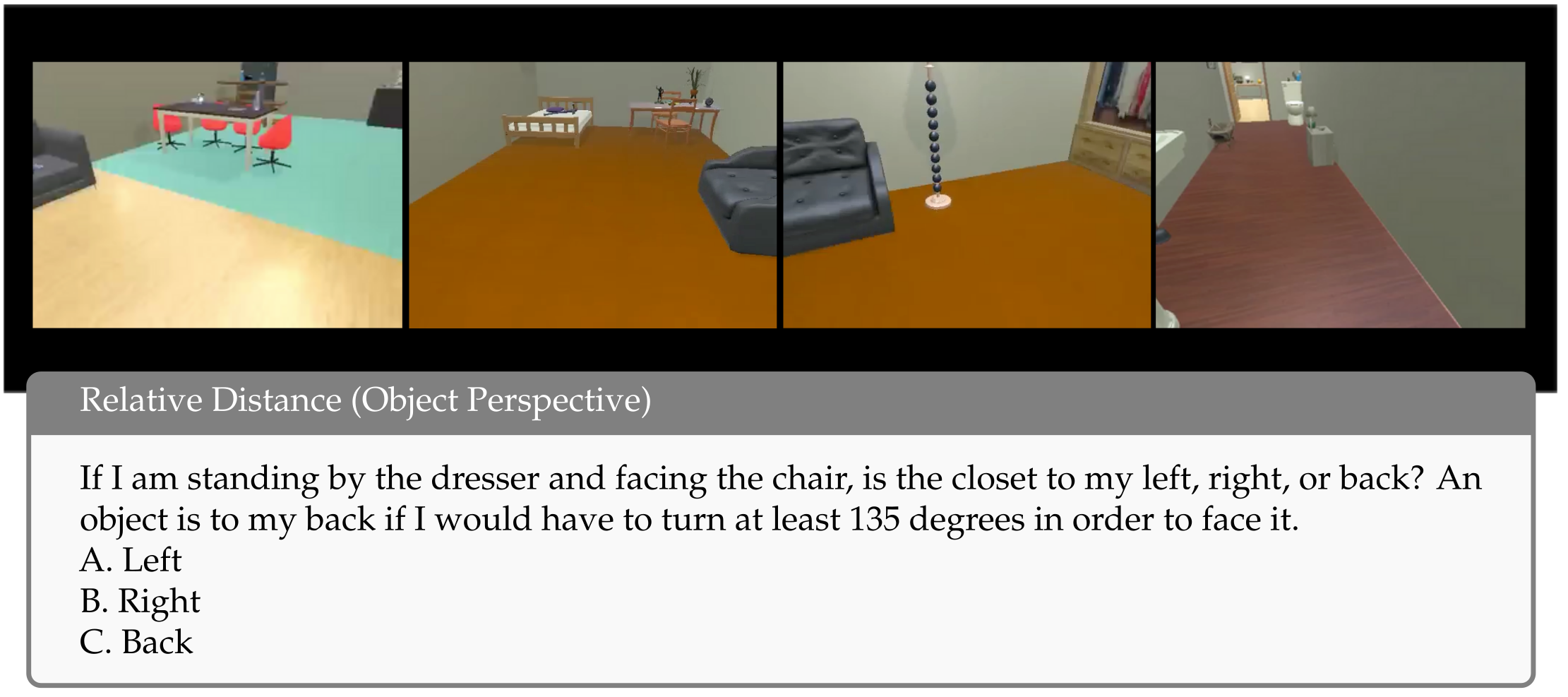
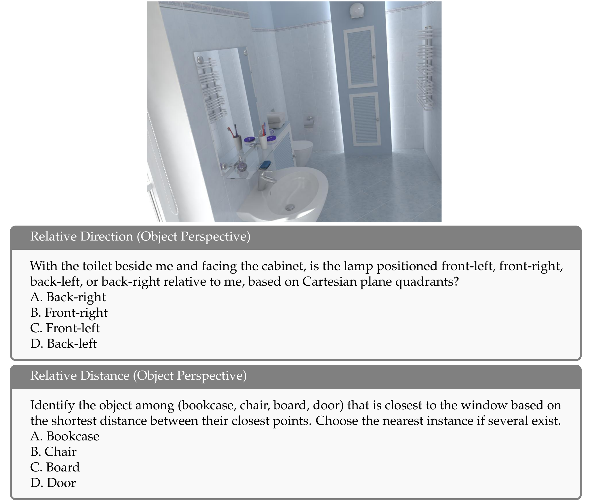
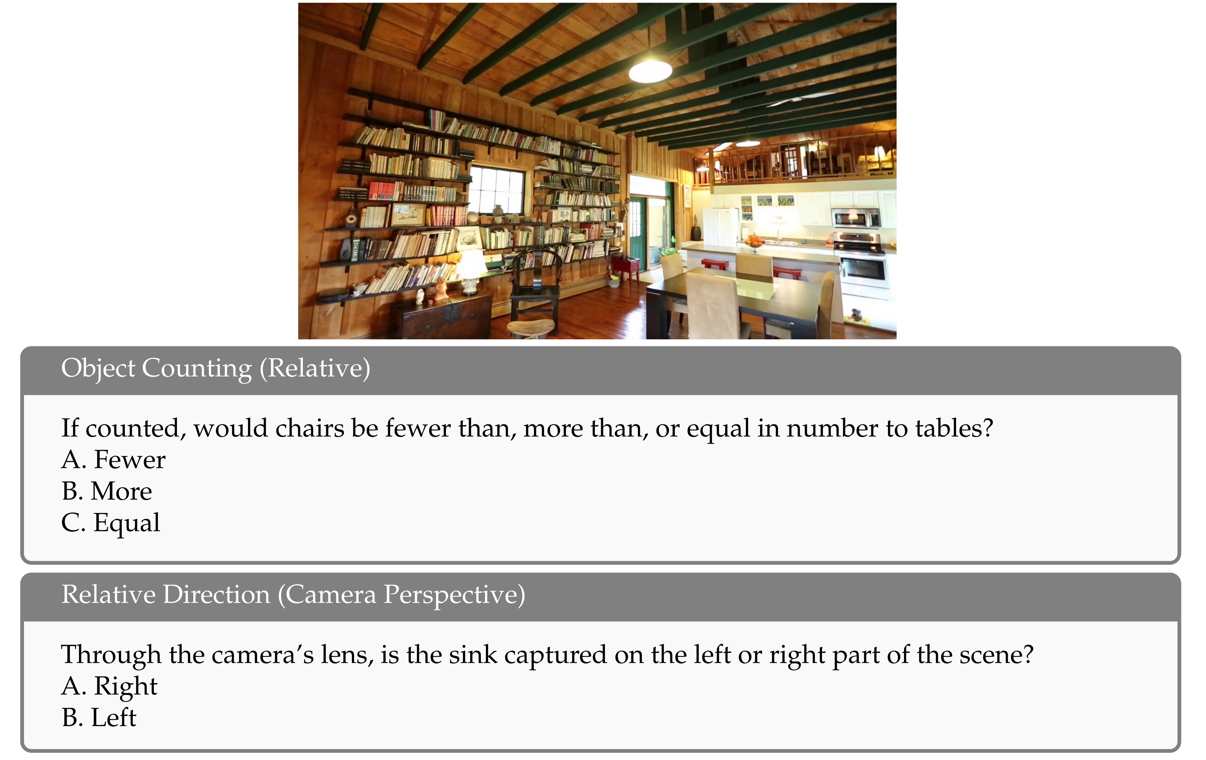
Figures 19–25 preserve real-video, simulated-video, and pseudo-annotated-image examples in full. Some source headings or templates are imperfect: Figure 19 labels a size-comparison question “Absolute Distance,” and the bathroom example in Figure 23 includes an office-object distance question. These are retained source artifacts and caution against treating selected examples as proof of uniformly clean labels.
Appendix D Cambrian- S Implementation Details
Implementation details specify the multimodal modules, data mixtures, resolution and token budgets, and distributed training infrastructure.
D.1 Model Architecture
A frozen SigLIP2-So400M visual encoder feeds a GELU two-layer connector and instruction-tuned Qwen2.5 decoder. The connector replaces Cambrian-1’s spatial vision aggregator. The original visual encoder’s pretraining objectives are background to the architecture, not objectives retrained from scratch here.
D.2 Training Data Mixture
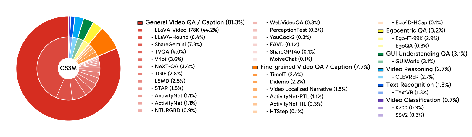
Stages one and two reuse Cambrian alignment and image instruction datasets. CambrianS-3M combines roughly three million open-source video QA examples, including general captions, fine-grained questions, ego-centric material, temporal localization, and interface interactions. Figure 16 retains the complete source composition. The final stage adds spatial specialization while retaining sampled general examples.
D.3 Training Recipe
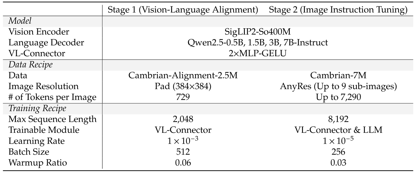
All four stages keep the visual encoder frozen. The connector alone learns alignment initially; subsequent stages also update the language decoder.
Stage 1: Vision-language alignment.
Alignment uses Cambrian-Alignment-2.5M, padded 384×384 images, a 2,048-token sequence limit, learning rate 10⁻³, and batch size 512. Only the connector is trained.
Stage 2: Image instruction tuning.
Image instruction tuning uses Cambrian-7M and an AnyRes strategy with up to nine 384×384 crops. The sequence limit expands to 8,192, learning rate drops to 10⁻⁵, and batch size is 256. The connector and language decoder are updated.
Stage 3: General video instruction tuning.
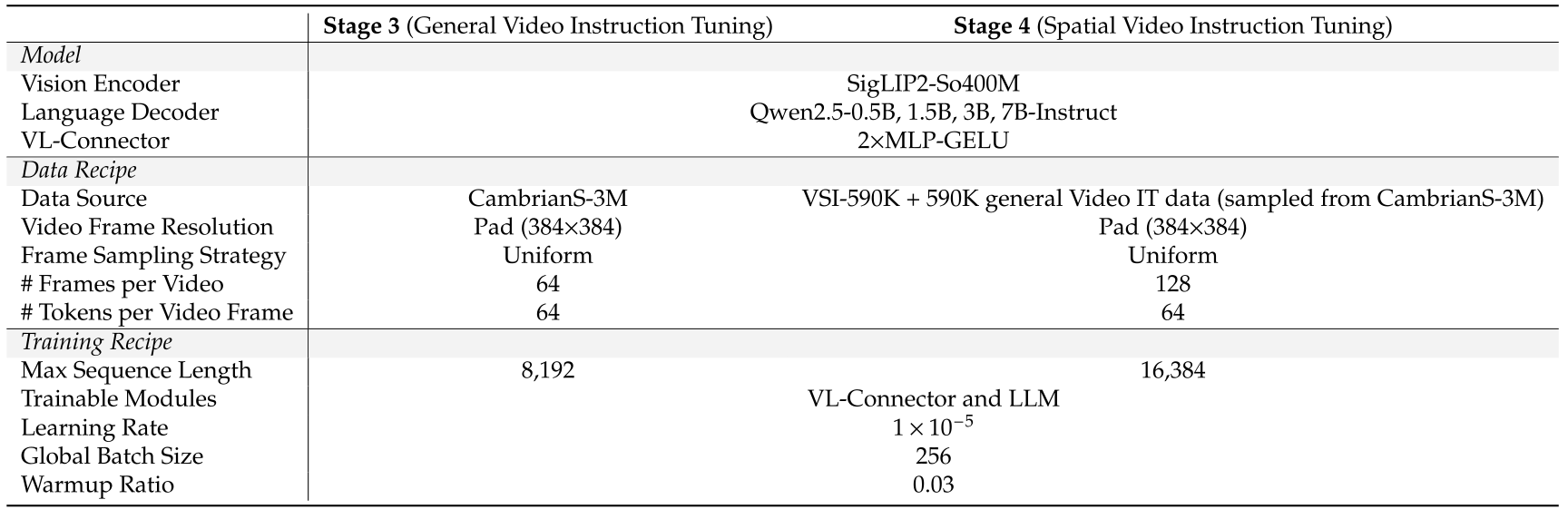
General video tuning mixes CambrianS-3M with sampled image examples. Each video supplies 64 uniformly sampled 384×384 frames, spatially reduced to 64 visual tokens per frame. Image handling follows the earlier resolution strategy.
Stage 4: Spatial video instruction tuning.
Spatial tuning mixes VSI-590K with 590K general-video examples and 120K image examples. It uses 128 frames and a 16,384-token sequence limit. The preserved configuration table lists learning rate 10⁻⁵ and global batch size 256. This recipe differs from the 1-FPS additional latent-prediction training subset.
D.4 Infrastructure
TPU v4 Pods, TorchXLA/GSPMD sharding, and Pallas FlashAttention support long-sequence training. The 7B model reaches a 16,384-token training length on a v4-512 Pod. These infrastructure details establish the reported setup, not a comparison of total training cost or energy efficiency.
Appendix E Cambrian- S Additional Results
Additional results expose benchmark-specific changes across stages, model sizes, image/video data proportions, and spatial versus general tuning.
E.1 Detailed Evaluation Setups
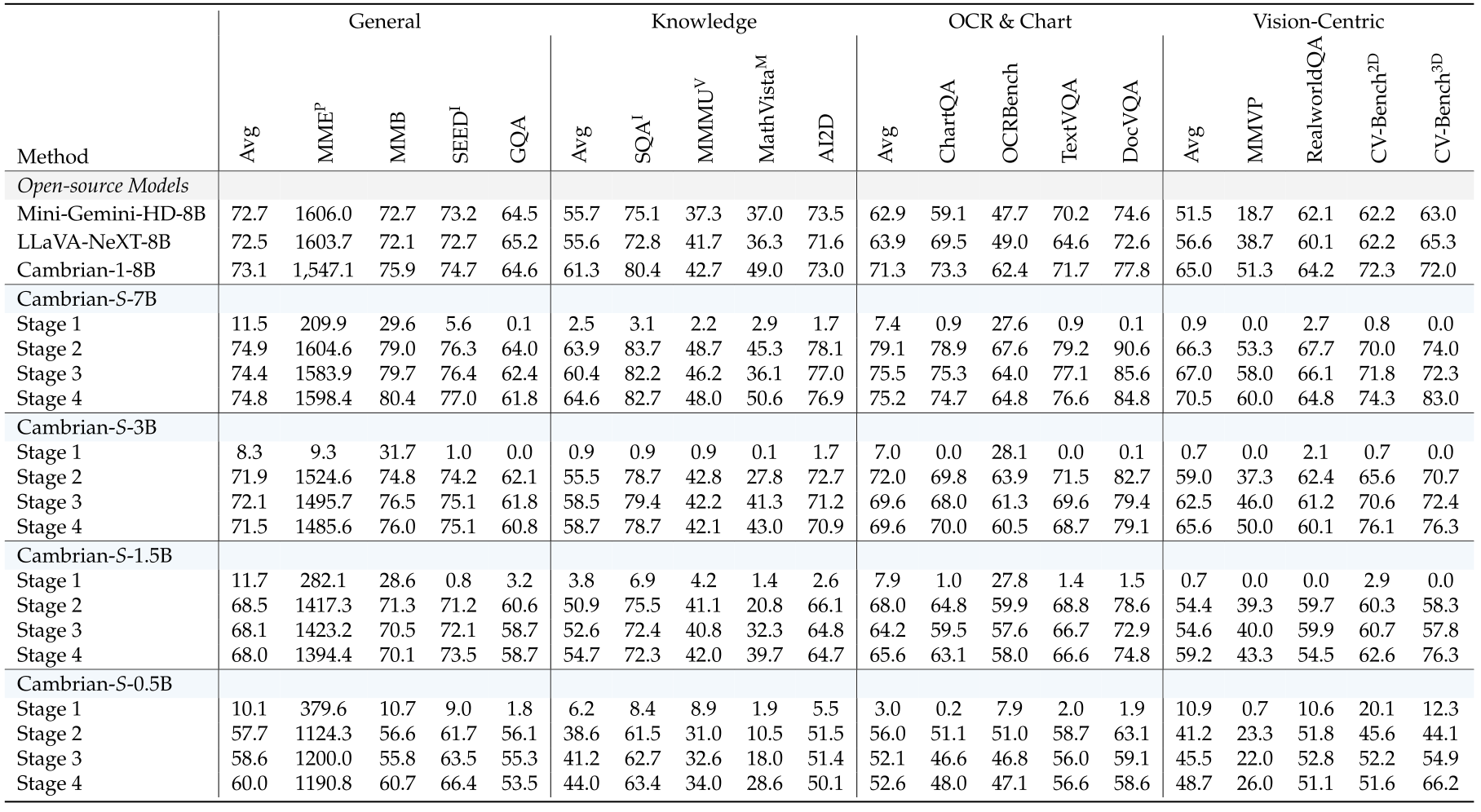
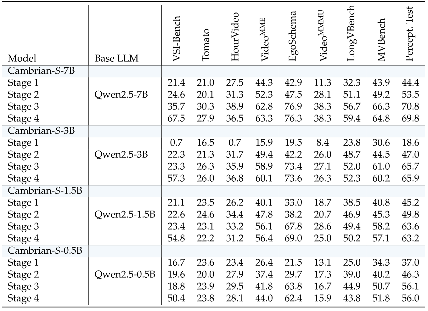
Standard image evaluation allows up to nine aspect-preserving 384×384 crops. Standard video evaluation uses 32 frames for stage-1/2 checkpoints, 64 for stage 3, and 128 for stage 4. Consequently, across-stage comparisons change both trained capabilities and available visual input; VSI-Super uses separate streaming protocols.
E.2 Detailed Performance on Image and Video Benchmarks
Tables 13–14 retain every checkpoint and benchmark score. The 7B spatial stage raises VSI-Bench from 35.7 to 67.5, while general results are mixed: VideoMME rises from 62.8 to 63.3, Perception Test falls from 70.8 to 69.8, and Tomato falls from 30.3 to 27.9. Small differences from headline tables are preserved rather than harmonized. “Without sacrificing general capabilities” is therefore an aggregate characterization, not improvement on every test.
E.3 Contributions from Image-based and Video-based Instruction Tuning
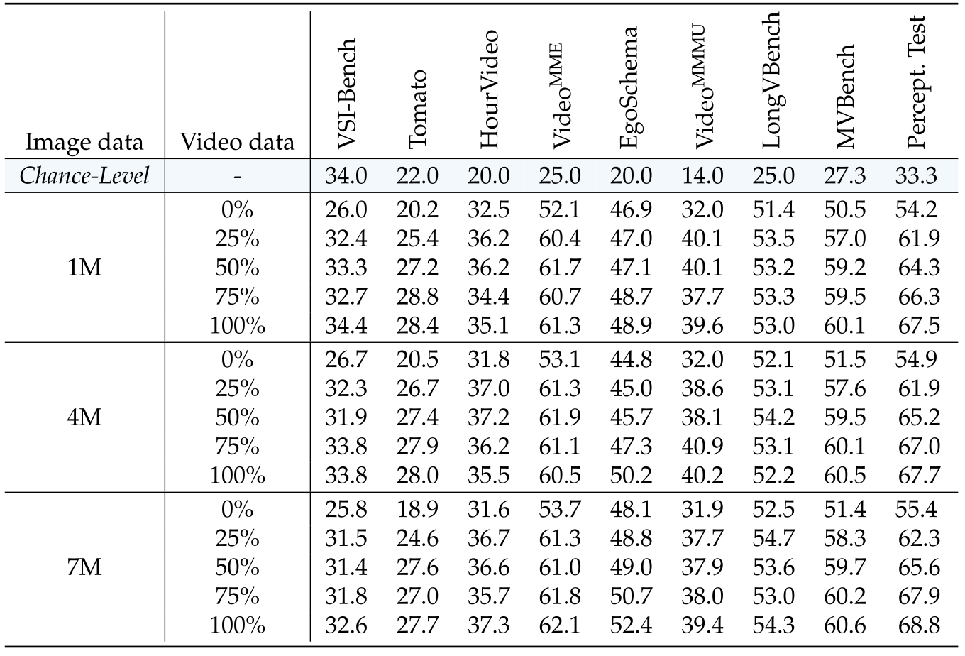
Models trained on 1M, 4M, or 7M images receive 25–100% of a video dataset. Even a quarter of the video data improves the tested image-only baselines, but further scaling is not uniformly beneficial. At full video data, the 7M-image model wins five of nine benchmarks. Data distribution and task alignment matter alongside size.
E.4 On the Trade-off between Spatial Sensing and General Video Understanding
Spatial-only tuning produces stronger VSI-Bench scores; mixed tuning better preserves general video performance across the plotted scales. The spatial gap narrows for larger models. The prose mentions a 1B scale here, while the model family and plotted labels use 1.5B; the original source displays are retained.
Appendix F Predictive Sensing
Predictive sensing combines auxiliary next-feature training with two different memory applications. Full original pseudocode is retained because scheduling, budget handling, and aggregation affect interpretation.
F.1 Latent Frame Prediction Implementation Details
The prediction head maps language-model hidden states to visual-feature dimension, with a tunable auxiliary loss contribution.
Latent frame prediction head.
Algorithm 2 gives the 7B head as Linear(3584,3584), GELU, and Linear(3584,1152), with biases. The 1152-dimensional output matches SigLIP2 features. The native code rendering preserves its exact nested structure and indentation.

On the balance between LFP and instruction tuning losses.
The default auxiliary coefficient is 0.1. Table 16 shows VSI-Bench changing from 67.5 without prediction loss to 66.1 at 0.1, 60.8 at 0.5, and 56.6 at 1.0. Prediction training therefore has a measurable specialization cost, with stronger weighting generally harming the reported spatial score. The table does not itself quantify long-memory gains at every coefficient.

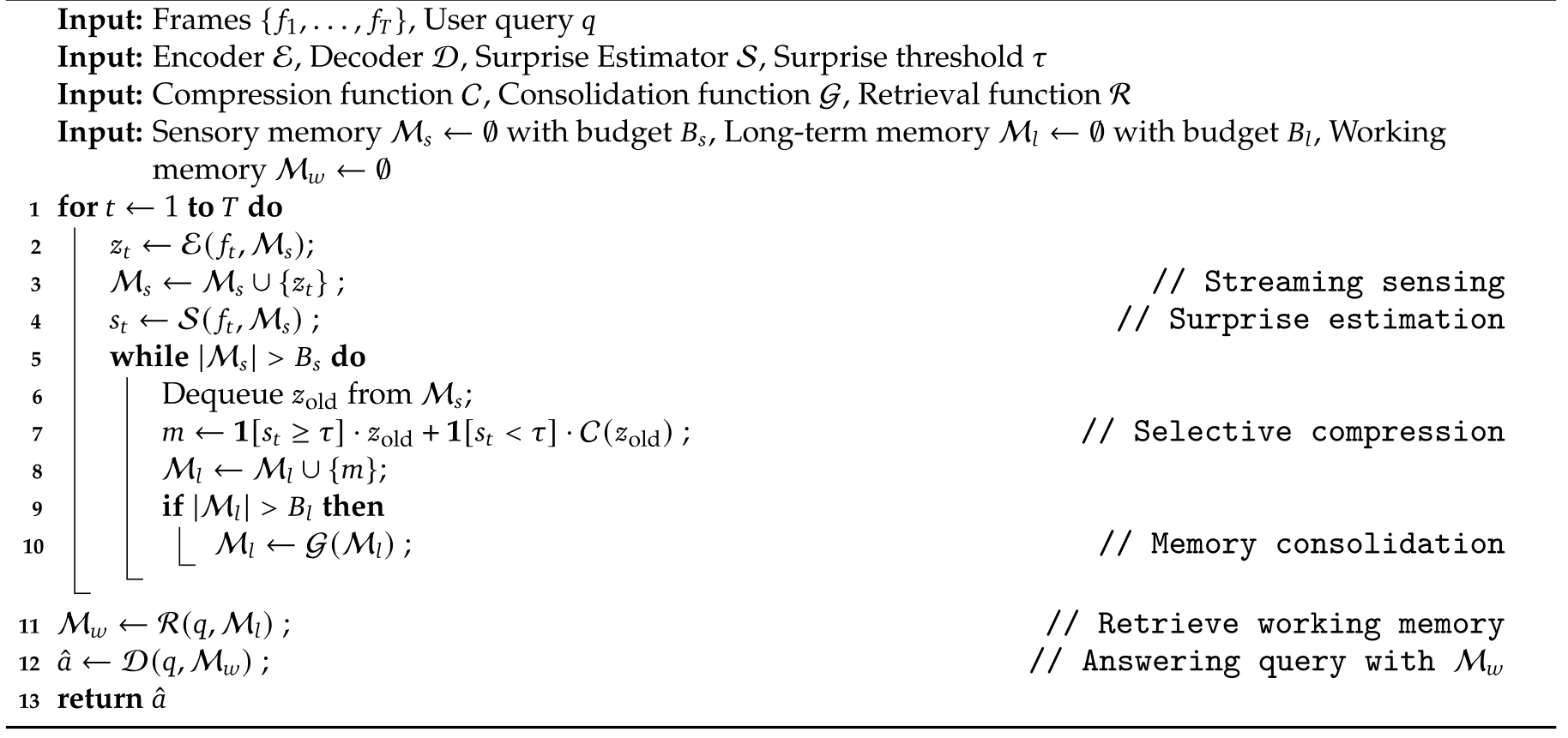
F.2 Memory Framework Design for VSI-Super Recall
Recall memory has sensory, long-term, and query-time working stores. Compression, consolidation, and retrieval operate on internal transformer caches rather than an external caption index.
Basic memory units.
Per-layer key/value pairs are the retained memory units. This lets retrieval reuse internal language-model attention representations, while making storage dependent on model layers and token counts.
Streaming sensing.
Each frame is visually encoded and then contextualized by the language model using a bounded recent sensory window. Frames leaving that window are candidates for long-term retention. The appendix denotes the window symbolically rather than supplying a complete fixed hyperparameter table.
Surprise-based memory compression.
A low surprise score triggers factor-two spatial downsampling of the outgoing frame’s cache. This selectively reduces stored detail. The prose assigns a surprise score to each frame, while Algorithm 3 writes the current score alongside a dequeued older frame; their timing correspondence is not fully specified in the paper.
Surprise-based memory consolidation.
An example long-term budget is 32,768 tokens. Consolidation repeatedly removes low-priority memories until below budget. Three strategies are discussed: forgetting the oldest, forgetting the least surprising, or combining least-surprising removal with adjacent surprising-memory merges. Exact default choices and all thresholds are not comprehensively tabulated.
Retrieval.
For each transformer layer, query features are compared by cosine similarity with cached frame keys, treating multihead features as one vector. The top-K frames provide key/value context for answering. Retrieval is query-conditioned after passive storage, so information discarded earlier cannot be recovered simply by selecting a different query.
F.3 Agentic Framework Design for VSI-Super Count
Algorithm 4 accumulates older frames in event memory, answers on high surprise, clears that store, and sums intermediate answers. Its pseudocode does not explicitly flush the final event or remaining sensory window at end-of-stream, and the prose does not resolve that edge case. The reported implementation may handle it elsewhere, but the paper alone does not establish how. Summation also assumes event counts can be combined without cross-event duplicate identities.
F.4 Comparisons with Existing Long-video Methods
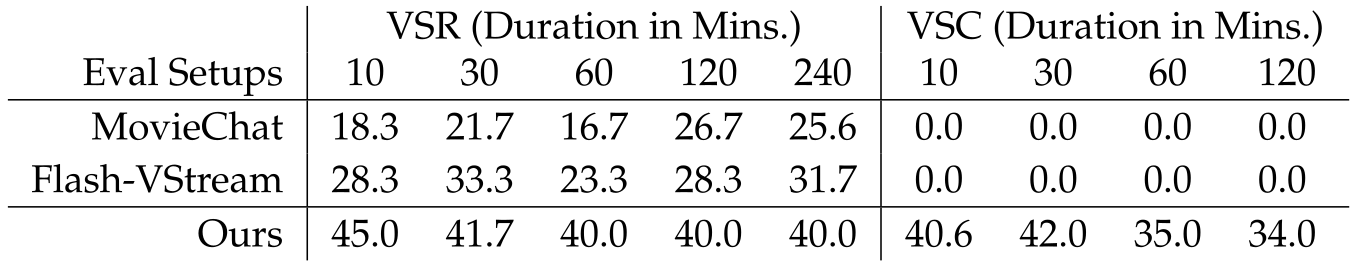
All compared memory strategies use the same LFP-tuned Cambrian-S-7B. MovieChat uses long-/short-memory budgets of 64/16; Flash-VStream omits its learned abstract-memory module because that would require dedicated training. Their VSC scores are zero, while the proposed agentic method scores 40.6–34.0 across durations. The controlled backbone is useful, but the partial Flash-VStream adaptation is not a complete reproduction of its original trained system. VSR comparisons favor the proposed store across all reported lengths.