At a glance
Rainbow learns a distribution of alternative condition embeddings for an image generator. A GFlowNet samples edge-addition trajectories in a latent graph; an order-sensitive decoder turns each trajectory into an embedding, blended with the original condition. Reported natural-image, brain-MRI and chest-X-ray experiments improve several diversity/fidelity metrics. The evidence concerns these implementations and proxy measurements; it does not establish calibrated uncertainty, universal model compatibility or clinical reliability.
1 Introduction
A condition such as a sunset description or an age/sex pair leaves many image attributes unspecified. Rainbow targets this ambiguity in the condition representation instead of relying only on different diffusion noise or textual prompt expansion. It still samples both graph trajectories and diffusion noise: the contribution is a learned additional source of variation, not the removal of randomness.
The intended benefit is multiple plausible interpretations of one condition. The latent graph has learned edge embeddings, rather than predefined semantic or causal relationships. Its interpretation is explored after training by associating frequently selected edges with visible attributes.
2 Preliminary
The method combines reward-proportional graph sampling with conditional latent diffusion. These components serve different roles: graph sampling diversifies the condition, while diffusion produces the image.
2.1 Generative Flow Networks (GFlowNets)
A GFlowNet constructs an object through a sequence of actions. Nonnegative flows are trained so that terminal objects are sampled in proportion to their reward. Conservation equates incoming and outgoing flow at intermediate states. In Rainbow, the actions add edges to a trajectory until a fixed edge budget is reached.
2.1.1 Detailed Balance Objective
Equation 1 penalizes squared log-ratio discrepancies between forward and backward transitions weighted by their state flows, plus a terminal reward-matching term. The balance concerns these weighted quantities; forward and backward probabilities need not themselves be equal. This is the Detailed Balance objective described by the method and Appendix C, following GFlowNet foundations.
Equation 1
| (1) |
2.1.2 Capturing Diversity with GFlowNets
Reward-proportional sampling can retain several high-reward modes instead of selecting only a maximum. An amortized stochastic forward policy then generates trajectories without a separate local Markov-chain search for every sample. These are the intended properties of a correctly learned flow; finite training and a denoising reward do not guarantee complete semantic coverage or calibrated uncertainty.
2.2 Latent Diffusion Models
A latent diffusion model encodes images into a compressed space, learns to predict added noise conditioned on a prompt, and decodes a denoised latent back to pixels. Equation 2 is the noise-prediction loss. Rainbow modifies the condition embeddings supplied to this process; it does not replace the image autoencoder or diffusion sampler.
Equation 2
| (2) |
3 R a i n b o w
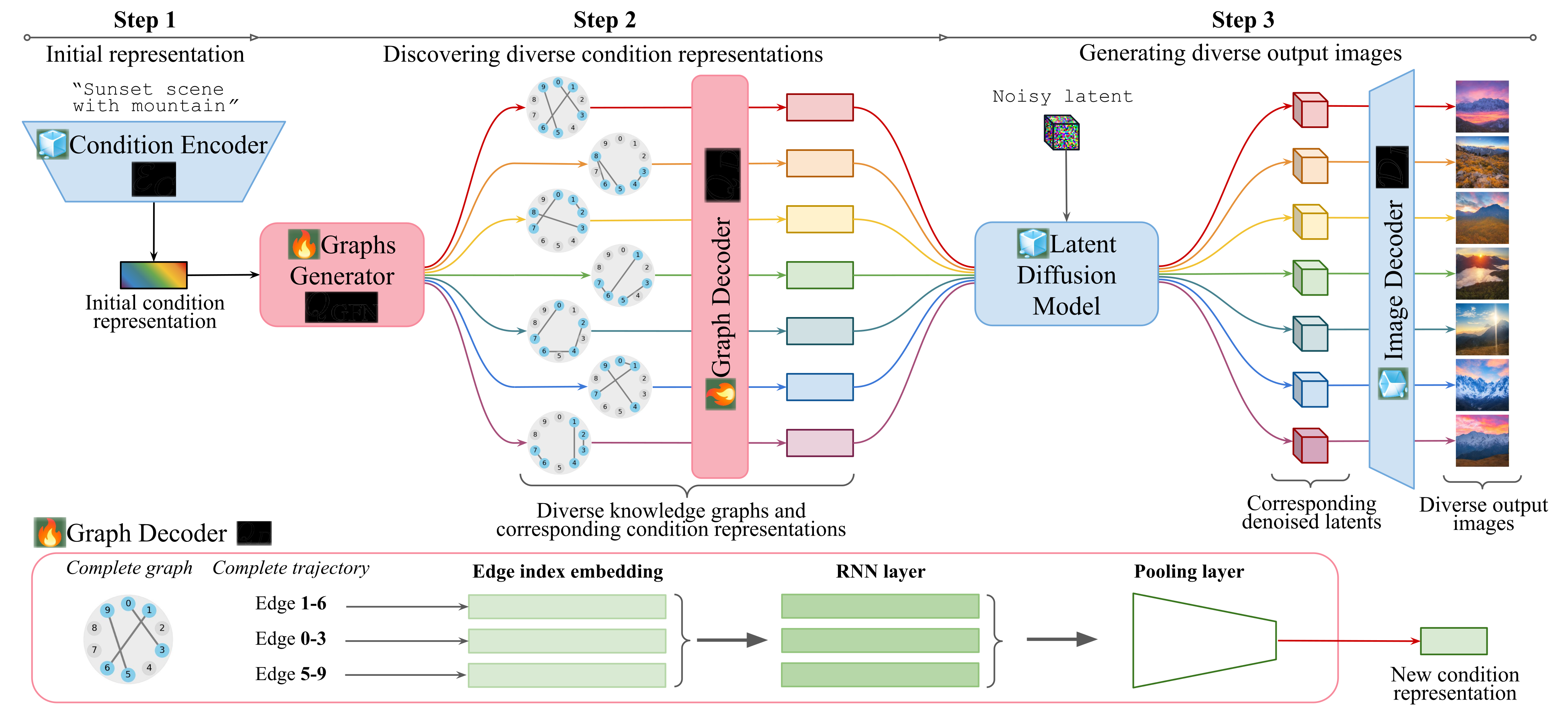
The graph generator and graph decoder sit between the original condition encoder and the image generator. Their purpose is to turn one condition into multiple related representations, each used to generate an image.
3.1 R a i n b o w ’s Inference Pipeline
Encode the input condition, sample M edge trajectories, and decode each to a condition embedding. Each embedding is paired with an independently sampled noisy image latent before diffusion and image decoding. The graph paths are stochastic samples, so the procedure does not enforce that every output or trajectory is distinct.
Equations 3–4
| (3) |
| (4) |
3.2 R a i n b o w ’s Training Details
Graph construction. Start with an undirected complete graph of N nodes and N(N−1)/2 possible edges. Each of the M trajectories starts with index 0 and adds edges until reaching S=(1−ρ)N(N−1)/2. Masks prevent repeated edges within a trajectory. The stated S+1 states describe one trajectory’s stages, not the entire combinatorial state space.
Decoding. Embed edge indices, process their sequence with an RNN, and pool/project to the original condition shape. Equation 6 blends this output with the original embedding using γ, set to 0.5 in the reported configurations. The RNN makes the representation dependent on edge order; it is not simply an unordered graph statistic.
Learning. A reward exponential in negative denoising MSE trains the GFlowNet, while denoising loss trains the graph decoder; α and β weight the two losses. The text specifies frozen pretrained components for natural images and chest X-rays, but the MRI experiment additionally fine-tunes its LDM. No separate explicit pairwise diversity penalty appears in the stated objective.
Equations 5–9
| (5) |
| (6) |
| (7) | ||||
| (8) | ||||
| (9) |

4 Experiment
Three questions organize the experiments: whether graph-conditioned sampling improves diversity, whether groups of edges can be interpreted, and whether generated images help downstream tasks.
4.1 Experiment Setup
Natural images: train on Flickr30k using frozen SD2-1 components, with M=40, N=20, S=32. Compare SD2-1, a baseline labeled “SD3.5,” CADS, and PAG; Table 3 also lists DDIM. The text and checkpoint link identify the “SD3.5” baseline as Stable Diffusion v3-medium, so its exact naming is inconsistent.
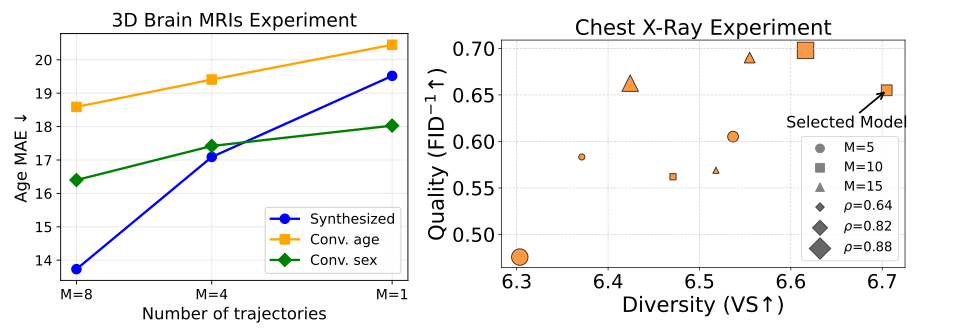
Brain MRI: roughly 27,000 scans without diagnosed disease from five cohorts train an age/binary-sex-conditioned 3D LDM. Rainbow uses M=8, N=8, S=8 and fine-tunes that LDM. Chest X-ray: use roughly 170,000 CheXpert images with a frozen, previously fine-tuned SD1.5 backbone, M=10, N=20, S=33, compared with that backbone and RadEdit. Different baseline pretraining datasets complicate attributing all cross-model differences to the graph mechanism.
4.2 Experiment Results
Interpret the results by domain and metric. Diversity, condition adherence and image quality are related but distinct; a gain on one score does not establish all three or validate a medical image.
| FID score | Sex Classification Accuracy | Age MAE | ||||||||||||||||
| Real data | 1e-5 | 96% | 3.55 | |||||||||||||||
|
|
|
|
|
|
|
|
| ||||||||||
| Random | - | - | - | 48% | 32.17 | |||||||||||||
| GAN Goodfellow et al. (2014) | 2.3329 | - | - | 63% | - | - | 29.23 | - | - | |||||||||
| LDM Cardoso et al. (2022) | 0.3288 | 0.3570 | 0.3590 | 68% | 68% | 67% | 21.52 | 20.35 | 19.43 | |||||||||
| Rainbow (Ours) | 0.3149 | 0.3375 | 0.3285 | 79% | 80% | 73% | 13.73 | 18.59 | 16.40 | |||||||||
4.2.1 Diverse Images Generation Results
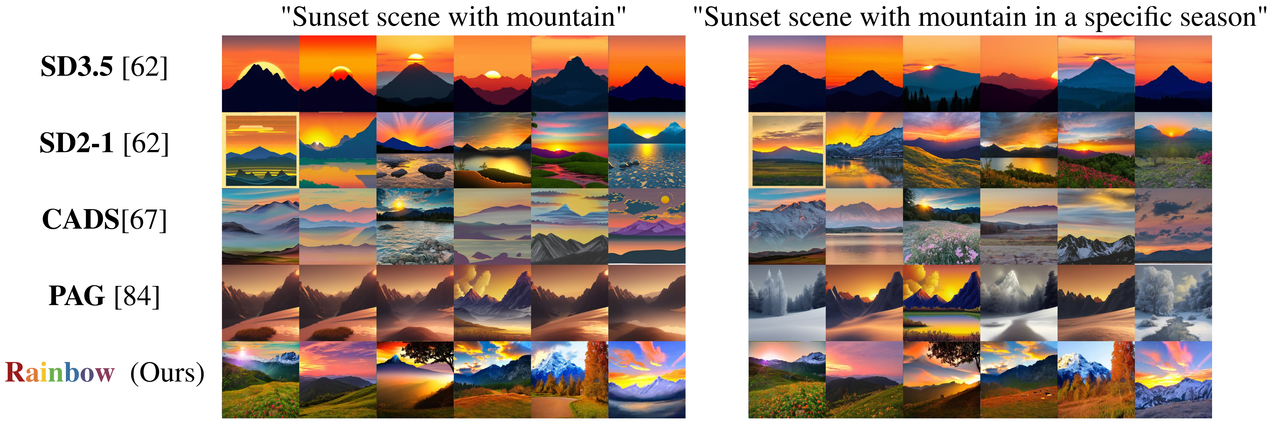
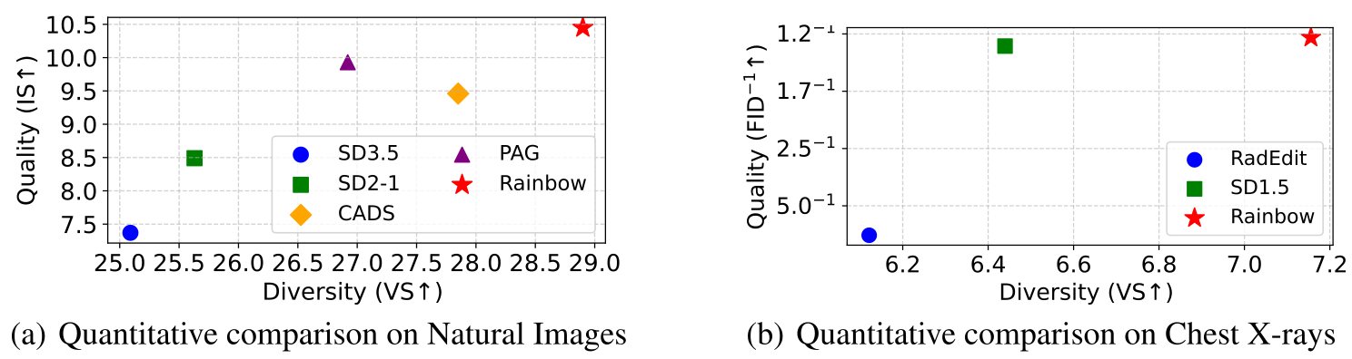
Natural images: 60 COCO validation prompts produce 40 images each. Rainbow scores 28.90 on Inception Vendi and 10.45 on Inception Score, versus CADS 27.85/9.46 and PAG 26.92/9.93. CLIP scores are close, about 30.3. The Vendi and Inception metrics measure feature diversity and classifier-based properties, rather than independently judged completeness of prompt interpretations.
MRI: on synthesis, Rainbow versus LDM reports FID 0.3149 versus 0.3288, sex classification 79% versus 68%, and age MAE 13.73 versus 21.52 years. Age- and sex-conversion results also improve in Table 1. However, real-data predictors achieve 96% and 3.55 years, leaving a substantial gap between generated and real images. These proxy comparisons do not establish anatomically valid individual counterfactuals.
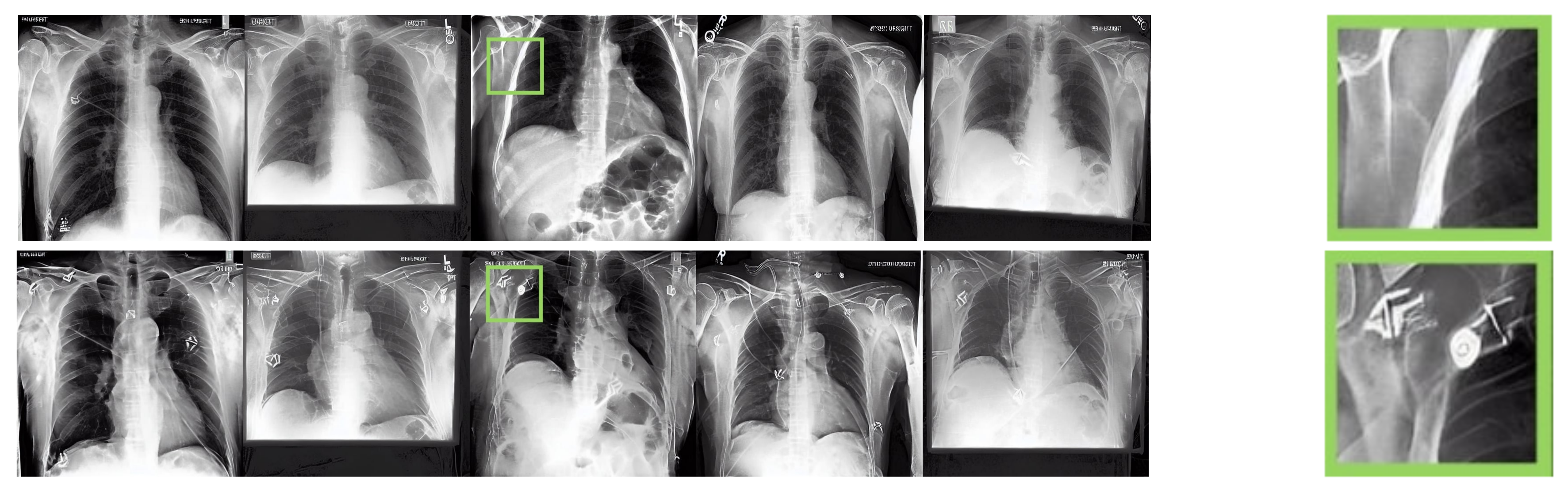
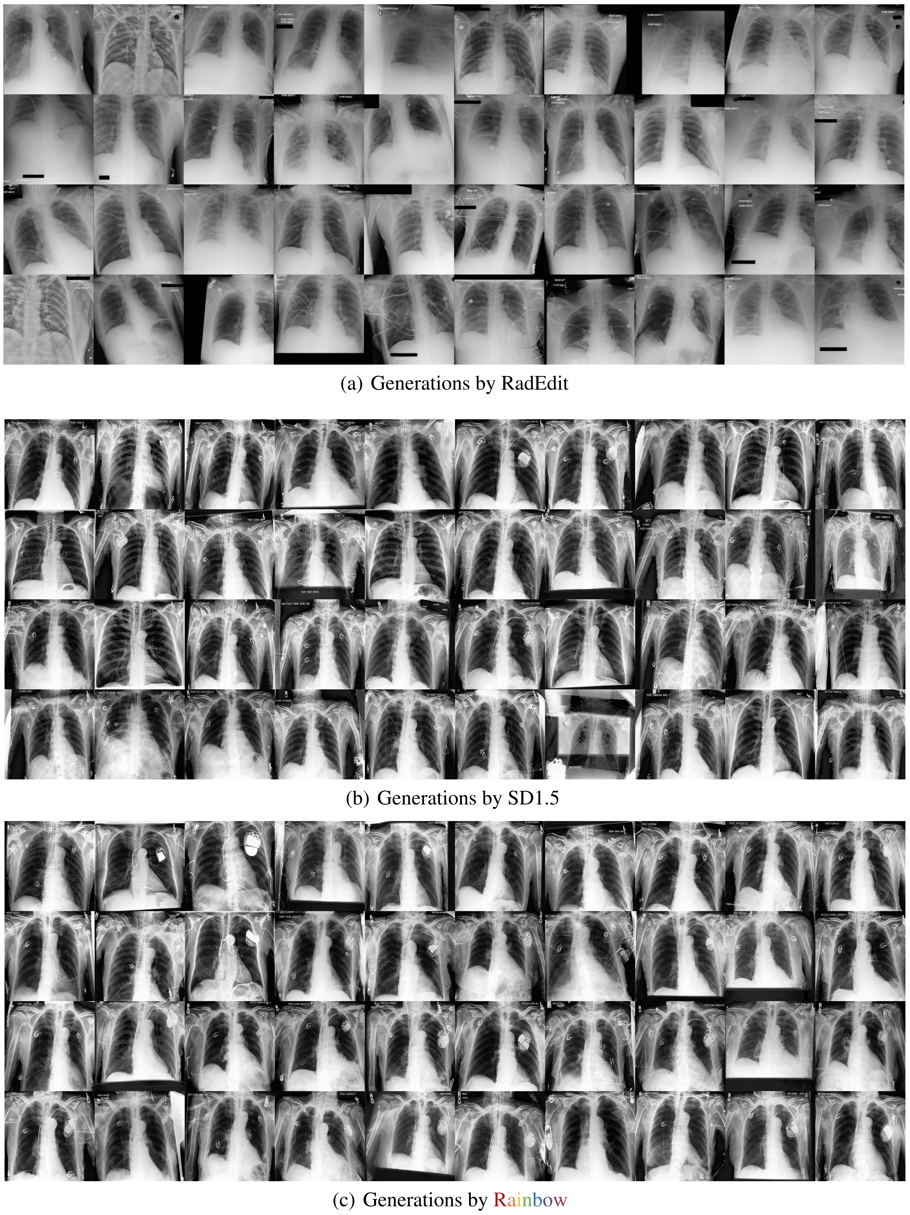
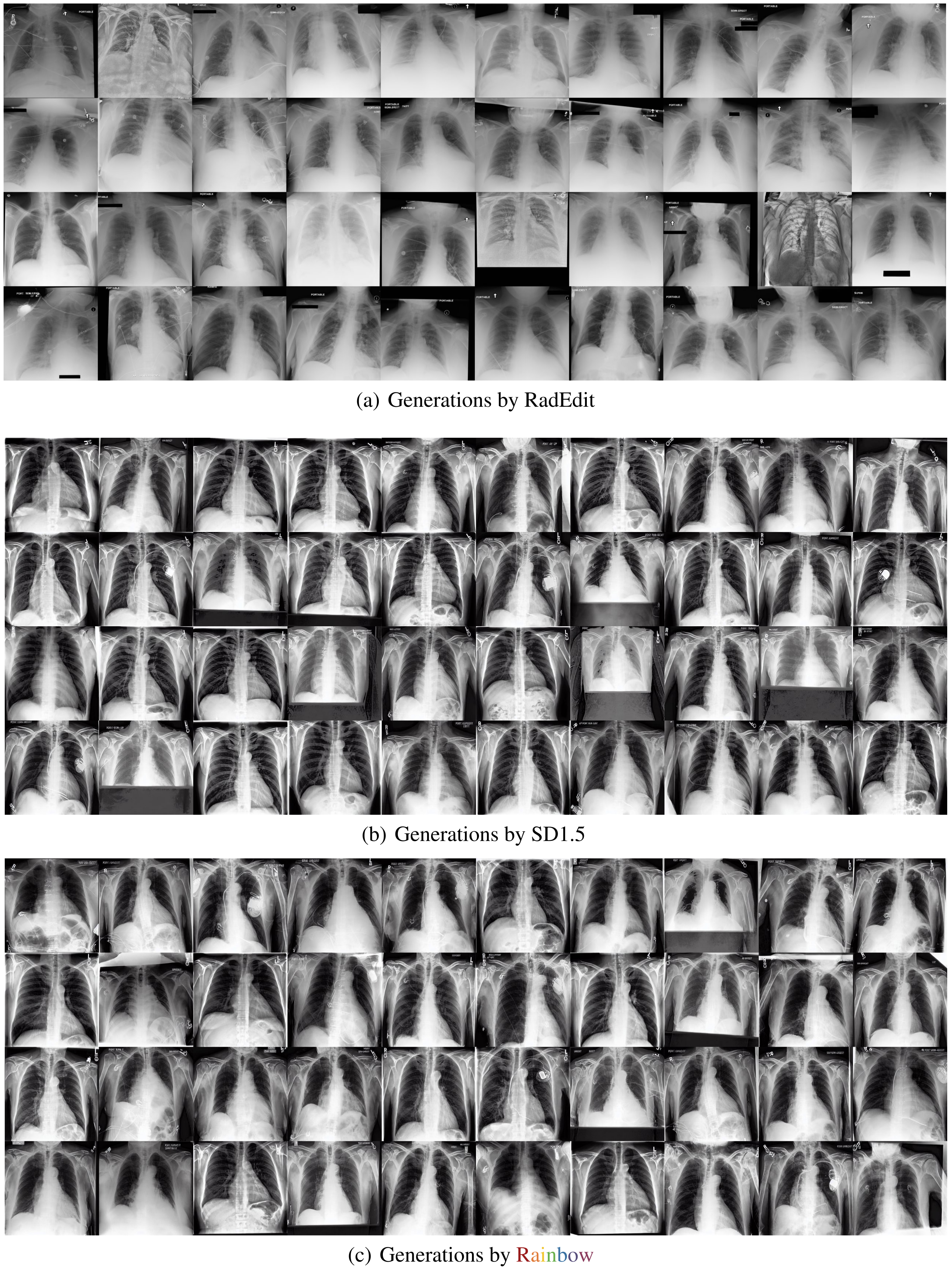
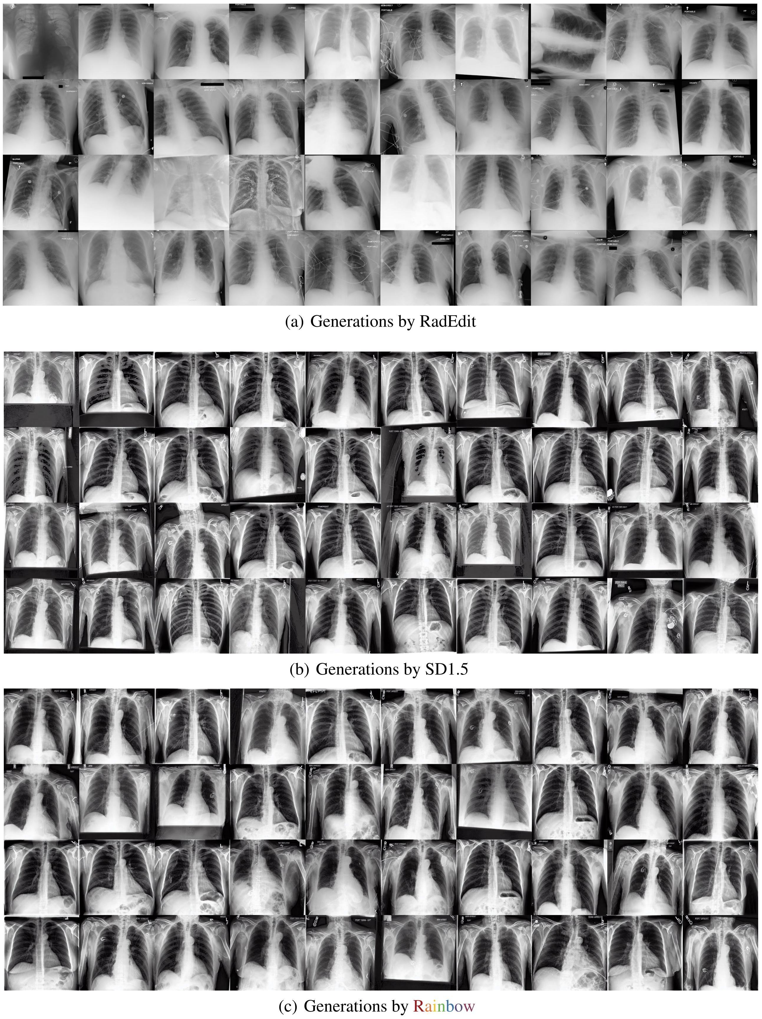
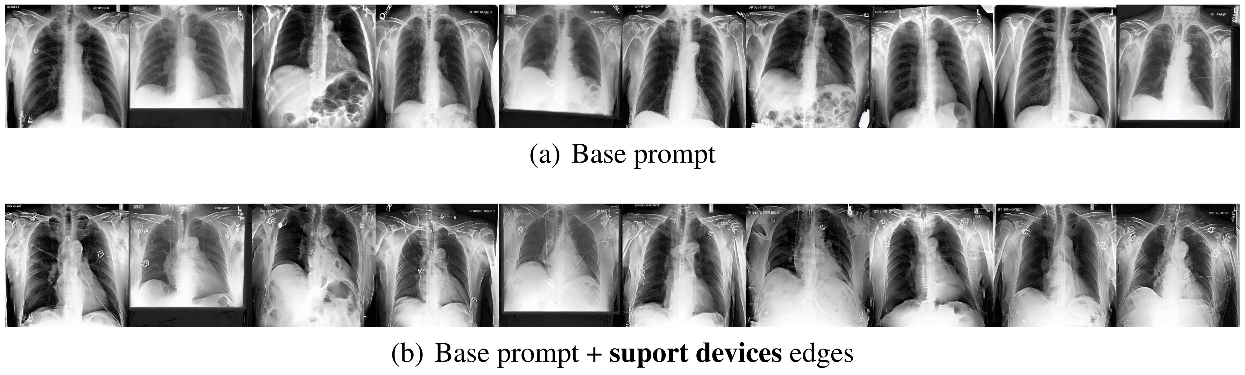
X-rays: Rainbow versus fine-tuned SD1.5 gives Vendi 7.16 versus 6.44 and FID 1.27 versus 1.32. CLIP is slightly lower, 33.45 versus 33.51; RadEdit gives 33.58. The galleries illustrate varied devices and anatomy. Their selected examples should not be read as a diagnostic accuracy assessment.


4.2.2 Latent Graph Interpretation
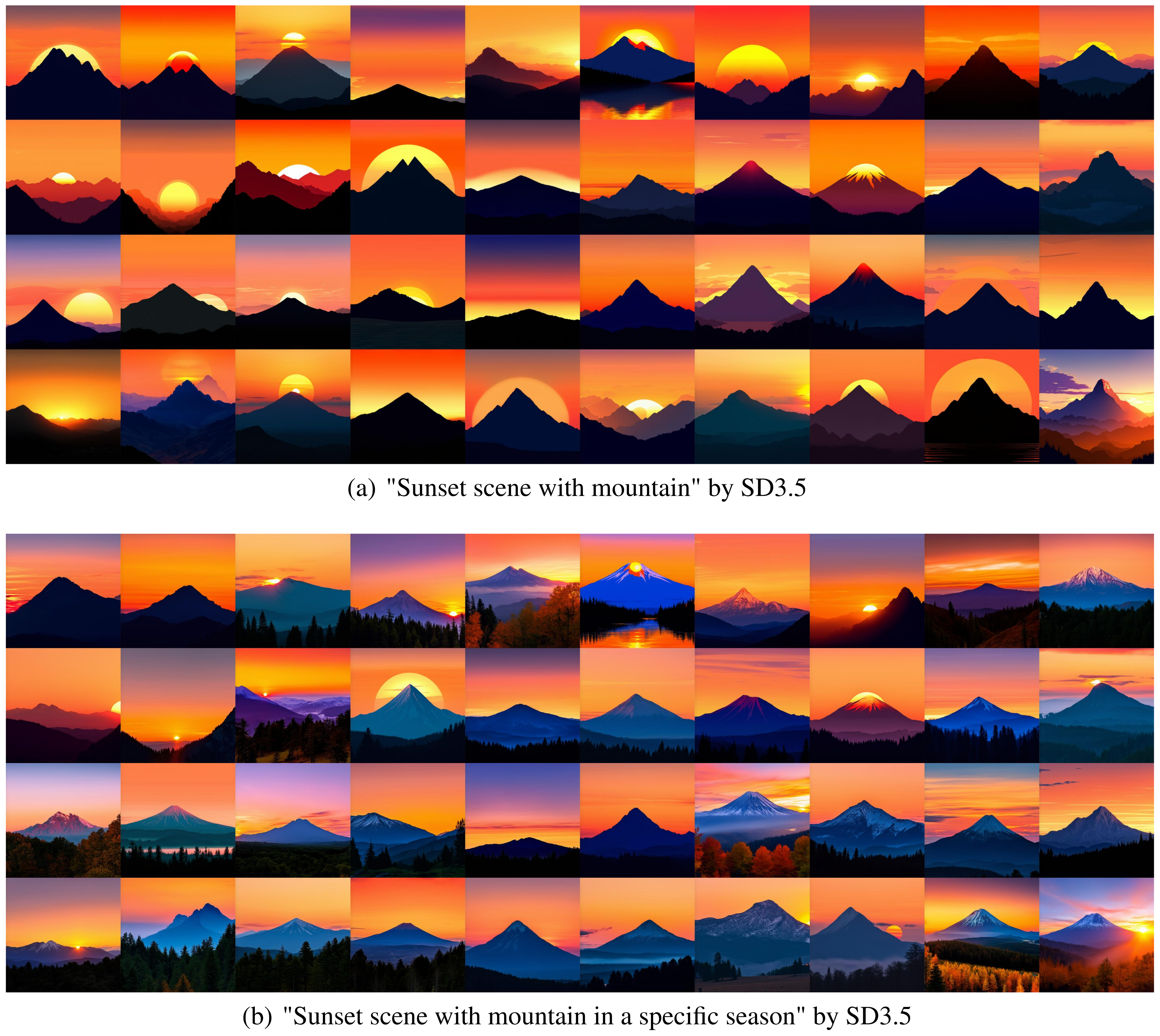
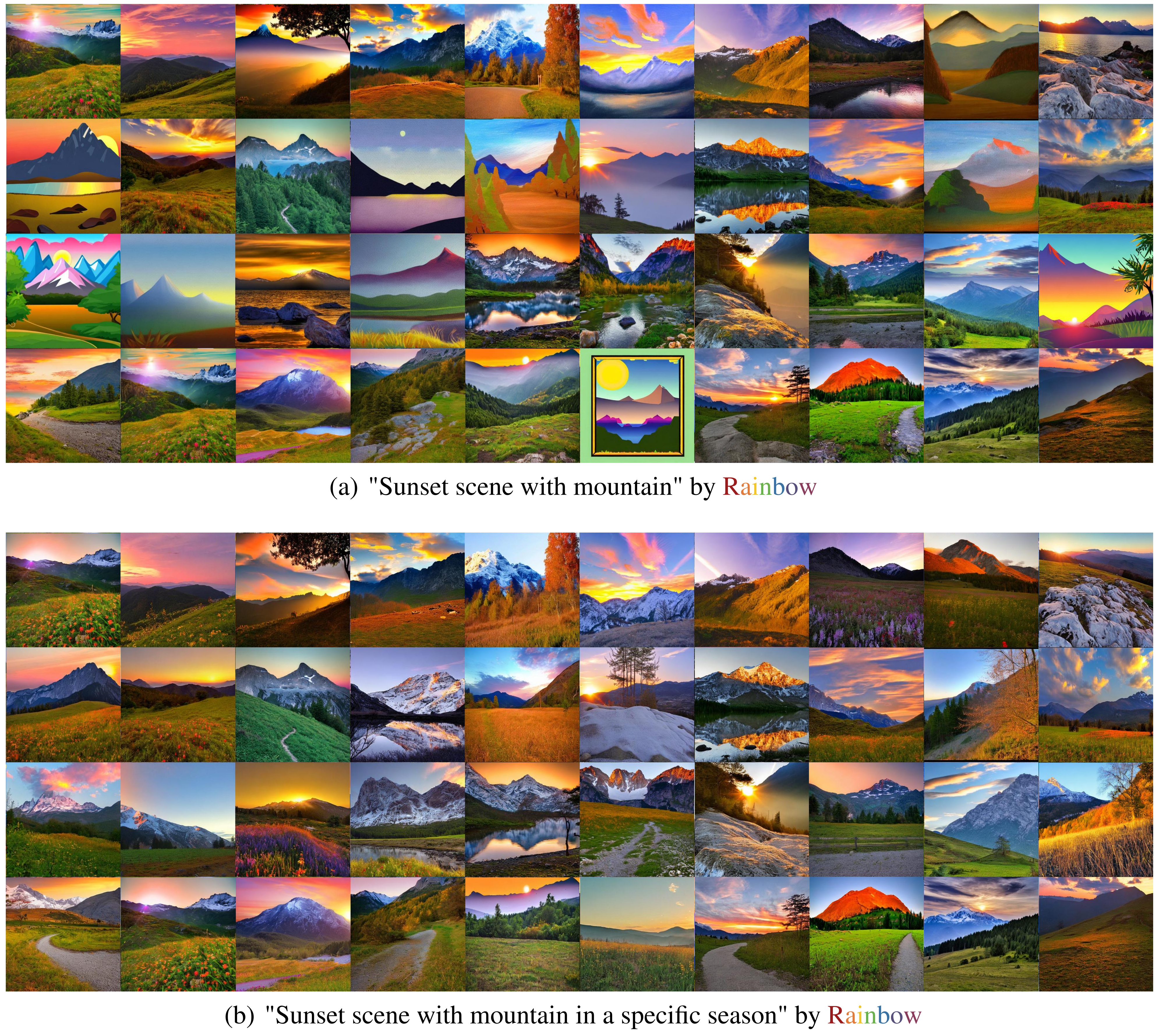
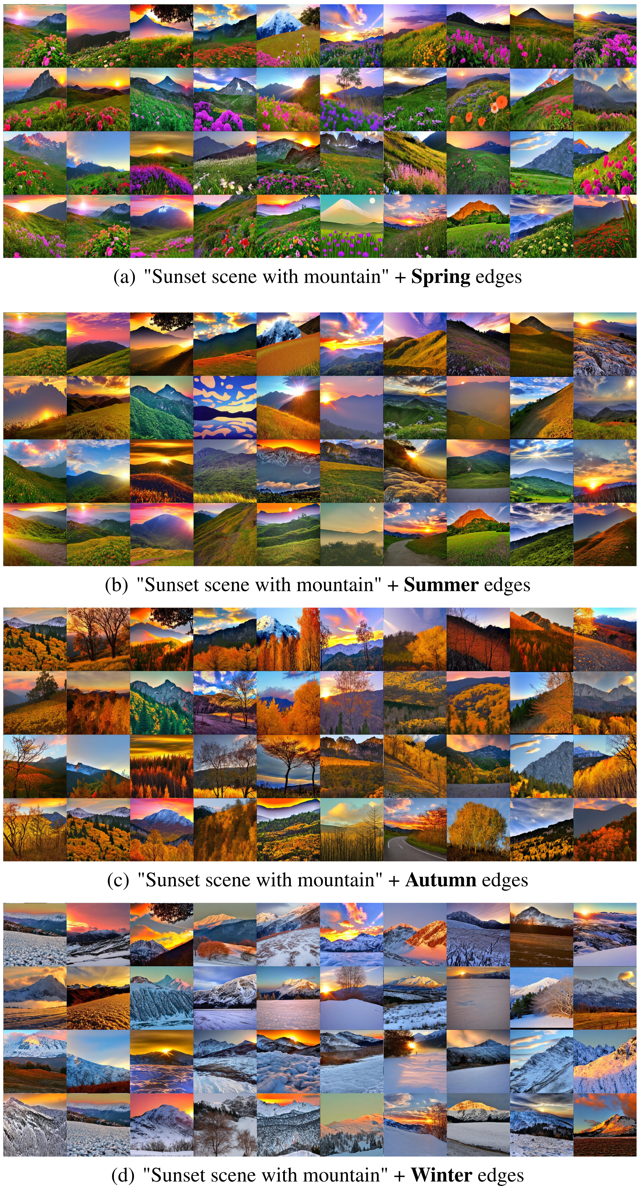
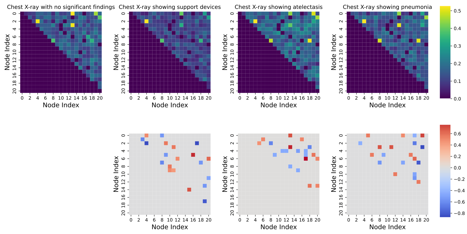
Cluster generated scenes by visible season, identify ten frequently added edges for each cluster, and append them to base trajectories. Resulting images often acquire flowers, autumn colors or snow while retaining some layout. A similar comparison of X-ray prompt trajectories identifies support-device edges. This demonstrates an empirical association and controllable perturbation of learned representations, not a predefined knowledge graph or proof of disentangled causal factors.
4.2.3 Performance on Downstream Tasks
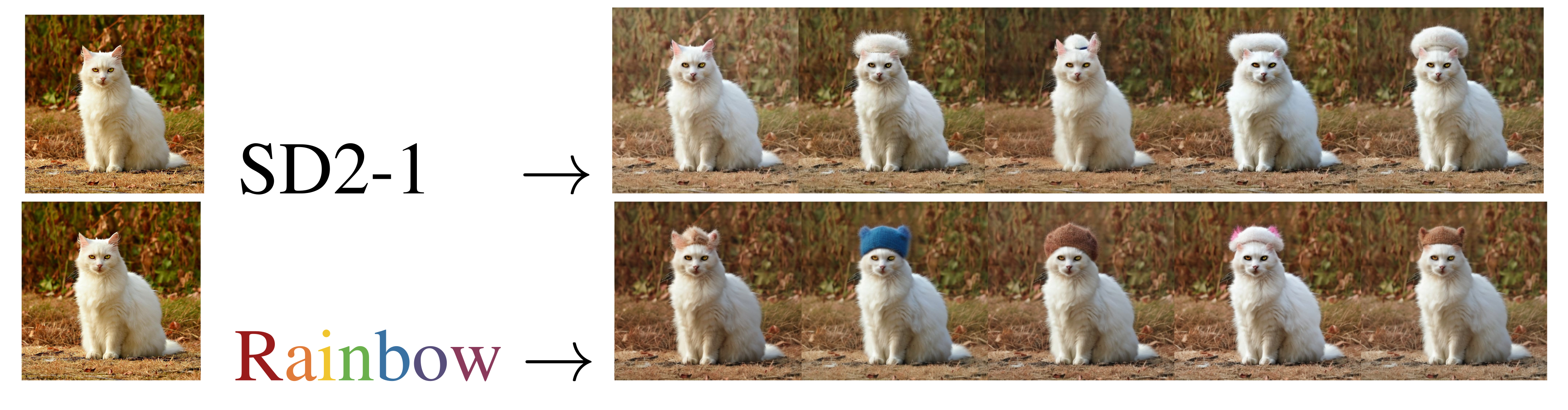
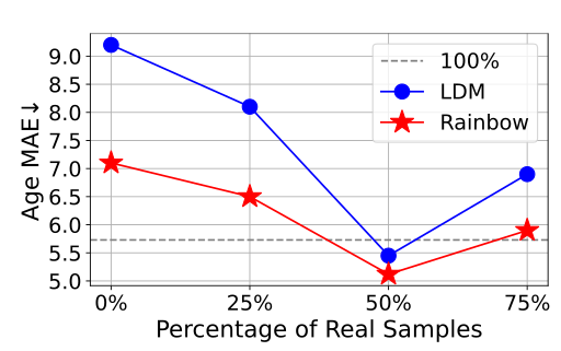
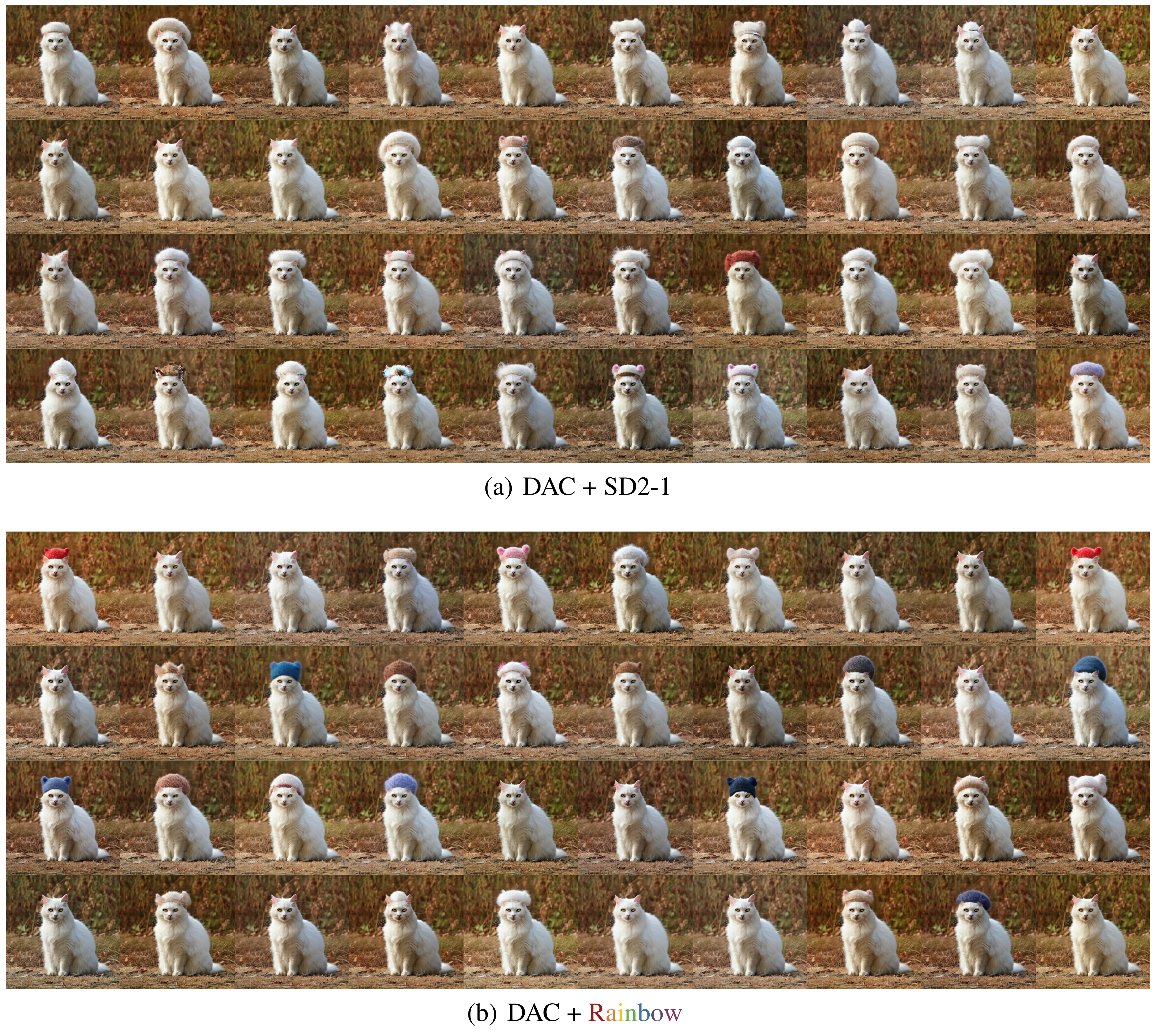
With the DAC editing pipeline, a wool-cap example produces more cap colors than the SD2-1 comparison. For MRI age prediction, the experiment uses 1,600 generated samples and varying proportions of real samples. Figure 9 shows the best reported MAE at a 50% real mixture for both generators, with Rainbow lower. The 100% reference is only 1,600 real examples, not a claim that synthetic data surpasses all available real data. The paper gives no independent clinical evaluation of the edited or augmented images.
4.3 Ablation studies
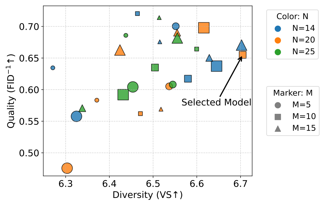
Increasing the number of sampled trajectories improves the reported MRI comparisons over M=1; the selected MRI configuration uses eight. X-ray diversity and fidelity depend jointly on trajectory count and sparsity, with ten trajectories selected. These X-ray ablations train for 16,500 steps, compared with 24,000 for the fully trained model, so their values should not be pooled with the final benchmark.
5 Related Work
Rainbow builds on conditional diffusion, methods that trade diversity against fidelity, and reward-proportional GFlowNet sampling. CADS diversifies conditioning during sampling; PAG generates alternative textual prompts, while Rainbow modifies latent representations and also accepts demographic conditions. This section calls its objective “Trajectory Balance,” whereas the method, equations and Algorithm 1 specify Detailed Balance. The edition follows the explicit algorithm and preserves the discrepancy.
6 Conclusion
The contribution is a trainable latent-condition sampler with favorable reported diversity/fidelity comparisons in three image domains and exploratory edge manipulation. Stronger claims about general-purpose uncertainty, automatic semantic interpretation, clinical counterfactuals or transfer to arbitrary generators remain beyond these experiments.
Acknowledgement
The authors acknowledge research funding, computing support, cohort data access, and MRI preprocessing/harmonization assistance. The original bibliographic and attribution material is retained.
NeurIPS Paper Checklist
The checklist declares reproducibility, statistical reporting and future code/model release, and reports no crowdsourcing or core LLM use. These are author declarations. The supplied results do not specify repeated-run uncertainty or confidence intervals, and the appendix does not give a complete data-split protocol despite the checklist’s broader reproducibility claim. A release promise is not itself evidence that artifacts are available.
Appendix A Broader Impacts
Diverse synthetic data could support augmentation and exploration, while realistic images can also mislead. The authors specifically require expert validation of medical counterfactuals before downstream clinical use. Improvements on feature metrics do not demonstrate reduced demographic bias or establish patient-specific diagnostic fidelity.
Appendix B Limitations and Future Work
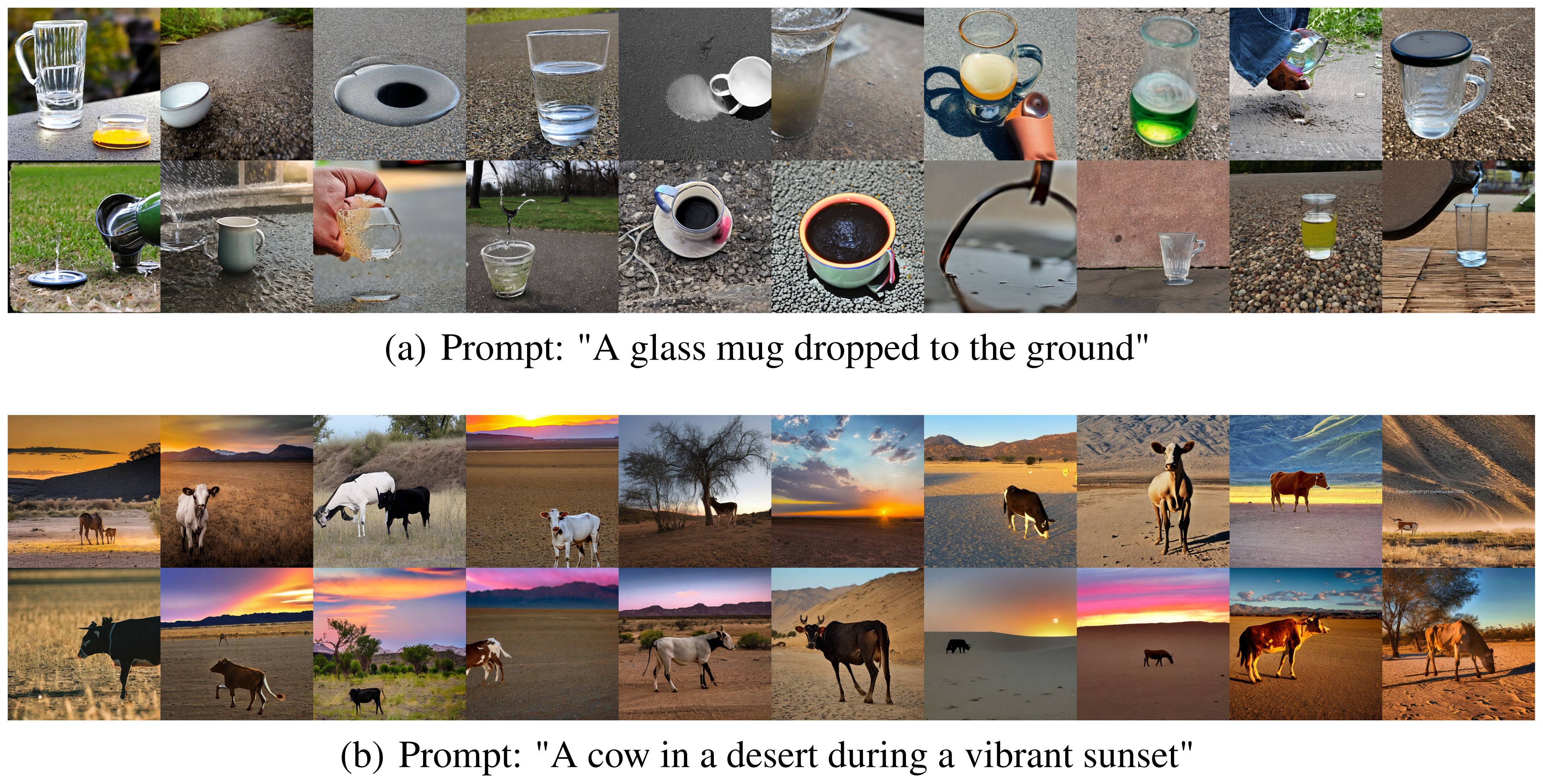
Parallel trajectories increase training cost, and semantic interpretation of the learned edges remains partly manual. Anatomical plausibility testing is explicitly left for future work. Text generation, recommendation, decision-making and larger “world model” graphs are proposed directions, not evaluated capabilities. Figure 21 retains failures on a dropped glass mug and a cow in a desert sunset, illustrating that broader variation does not ensure condition satisfaction.
Appendix C Further Computation Details
The appendix expands the diffusion and graph-training computations. It is useful for understanding the intended implementation, while several notation inconsistencies prevent treating the pseudocode as directly executable.
C.1 Conditional Image Generation with Latent Diffusion
Training encodes an observed image and condition, corrupts the image latent, and learns reverse denoising. Generation starts from a Gaussian latent; image editing instead starts from an encoded image, adds noise and denoises under a changed condition. The forward and reverse displays are preserved as printed. Calling the edited result a counterfactual describes the generative operation; it does not identify an individual’s real causal response to age or sex interventions.
Equations
C.2 GFlowNets Training
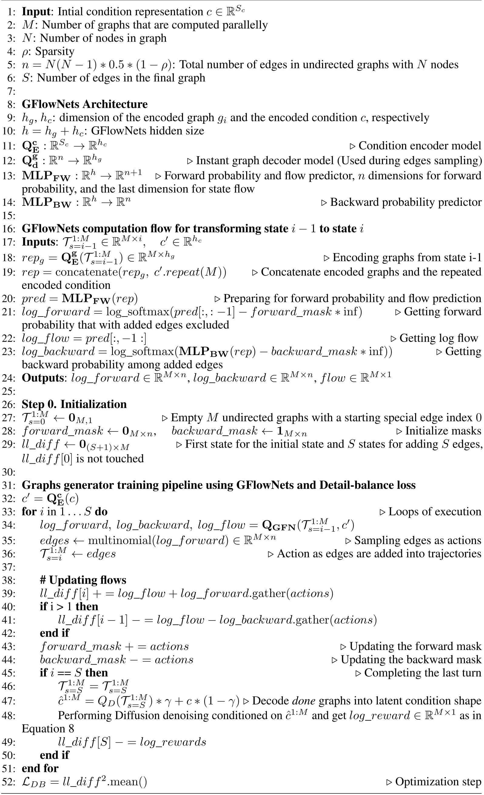
Algorithm 1 retains the full architecture, masks, edge sampling, flow accounting and reward update. It implements the intended Detailed Balance training rather than the “Trajectory Balance” label in Related Work.
C.2.1 Initialization Phase
Initialize M trajectories with the special starting index, a forward mask of zeros, a backward mask of ones, and an (S+1)×M residual array. The algorithm defines n with a sparsity factor while elsewhere n indexes possible edges and S counts selected edges; this distinction needs resolution in an implementation. The unused residual row 0 remains in the displayed mean.
C.2.2 Iterative Edge Sampling Phase
Encode the partial edge sequence and condition, concatenate them, and predict forward log probabilities, backward log probabilities and log flow. Masks exclude previously selected forward edges and invalid backward removals. Sampling adds one edge per trajectory and updates transition residuals. The printed pseudocode alternates edges/actions, passes log probabilities to a multinomial call, and uses a backward-update sign that needs checking against Equation 1. These are retained source ambiguities, not silently repaired code.
C.2.3 Finalization and Loss Computation Phase
Decode the completed sequences, blend them with the original condition, and obtain rewards through denoising. The last residual subtracts log reward, and mean squared residuals give the DB loss. The pseudocode also alternates singular/plural reward names. The training intent is clear, but reproduction requires resolving these notational details.
Equation
Appendix D Experiment Setup
Architecture, configuration, feature metrics, baselines and compute are specified below. Some implementation details and evaluation uncertainty remain unreported.
D.1 Hyper-parameter
All domains use γ=0.5 and RNN-based graph decoding. Natural images use three Rainbow epochs, learning rate 10⁻⁵ and 40 trajectories; MRI uses 80 pretraining epochs plus 20 Rainbow epochs, learning rate 2.5×10⁻⁶ and eight trajectories; X-rays use five epochs, learning rate 10⁻⁵, batch size eight and ten trajectories. MRI weights are α=0.2 and β=0.8; the other domains use 1/1 with frozen U-Net.
Table 2 is preserved exactly. Its X-ray setting N=20, ρ=0.82, S=33 is inconsistent with the stated formula, which gives 34.2 before rounding. The natural-image and MRI formulas likewise yield nonintegers, but their stated edge counts are consistent with rounding down; a general rounding rule is not supplied.
| Parameter Name | Natural Images | 3D Brain MRIs | Chest X-rays |
| Learning Rate | 1e-5 | 25e-7 | 1e-5 |
| Pretrained-LDM epochs | - | 80 | - |
| Rainbow epochs | 3 | 20 | 5 |
| Batch Size | 1 | 1 | 8 |
| 1 (Freeze Unet) | 0.2 | 1 (Freeze Unet) | |
| 1 | 0.8 | 1 | |
| Training image shape | |||
| Training condition type | Text prompt | Age and binary sexes | Text prompt |
| Training condition shape | Dynamic length | 2 dimensions | Dynamic length |
| Latent image shape | |||
| Latent condition shape | 256 | ||
| Inference image shape | |||
| Encoder - Decoder | VAE | VAE | VAE |
| Graph Size | 20 nodes | 8 nodes | 20 nodes |
| Number of Graphs | 40 | 8 | 10 |
| Sparsity | 0.83 | 0.70 | 0.82 |
| Num. Edges | 32 | 8 | 33 |
| Use RNN | Yes | Yes | Yes |
| Edge Embedding dim | 512 | 128 | 512 |
| Latent | 1024 | 1024 | 1024 |
| Blending factor | 0.5 | 0.5 | 0.5 |
D.2 Evaluation Metrics
Natural-image scores use Inception-v3 features. MRI FID uses 2,048-dimensional 3D ResNet50 features; age and sex are evaluated by CNN predictors trained on the real-data pool used for generation training. X-ray scores use 1,024-dimensional DenseNet-121 features from TorchXrayVision. These feature spaces differ, so absolute FID values should not be compared across domains. Feature similarity and condition-predictor accuracy remain proxies for perceptual or clinical correctness.
D.3 Baselines
The natural-image baselines include SD2-1, the inconsistently named SD3-medium/“SD3.5,” CADS and PAG; DDIM also appears in the quantitative table without equivalent setup detail. MRI compares a 3D GAN and a latent diffusion baseline. X-rays compare RadEdit, trained on a larger multi-dataset collection, with a CheXpert-fine-tuned SD1.5 model from PRISM. These are reported implementations, not a comparison to every model available in each domain.
D.4 Training Time and Computation Sources
Natural-image training takes 12 hours on one H100 80GB. MRI uses four H100 80GB GPUs and 32 CPU cores for three days of pretraining plus 24 hours of Rainbow training. X-rays use four A100 80GB GPUs and 24 CPU cores for 15 hours. These reported runs do not quantify all tuning cost or inference overhead, and parallel trajectory cost is an acknowledged limitation.
Appendix E Addition Experiment Results
The appendix retains all complete image grids, numerical tables, edge heatmaps and failure cases. The galleries complement aggregate metrics; they do not provide error bars or establish the frequency of every illustrated behavior.
E.1 Numeric Evaluation Results
Table 3 gives Rainbow the highest aggregate IS, pixel Vendi and Inception Vendi among the listed models, with nearly unchanged CLIP. Table 4 shows a larger diversity gain than FID gain over SD1.5 for X-rays, and slightly lower CLIP. Neither table supplies confidence intervals or repeated-seed variation, so small numerical differences should not be interpreted as established statistical significance.
| Model name | IS | CLIP | Pixcel VS | Inception VS |
| SD3.5 | 7.37 | 30.29 | 3.75 | 25.09 |
| SD2-1 | 8.49 | 30.27 | 3.74 | 25.63 |
| CADS | 9.46 | 30.27 | 3.88 | 27.85 |
| PAG | 9.93 | 30.21 | 3.90 | 26.92 |
| DDIM | 8.44 | 30.28 | 3.91 | 26.62 |
| Rainbow | 10.45 | 30.32 | 3.94 | 28.90 |
| Model name | FID | CLIP | VS |
| RadEdit | 10.28 | 33.58 | 6.12 |
| SD1.5 | 1.32 | 33.51 | 6.44 |
| Rainbow | 1.27 | 33.45 | 7.16 |
E.2 Chest X-Ray Ablation Studies
The partial-training sweep varies node count, trajectory count and sparsity together. Larger sparsity often favors Vendi, while lower sparsity favors FID; ten or fifteen trajectories generally improve over five. The blue node-count label is 14 in the plot but 15 in its caption, a source inconsistency. The selected model represents a chosen tradeoff rather than proof that one parameter setting dominates every metric.
E.3 Full of 40 Generations for General-domain Experiments
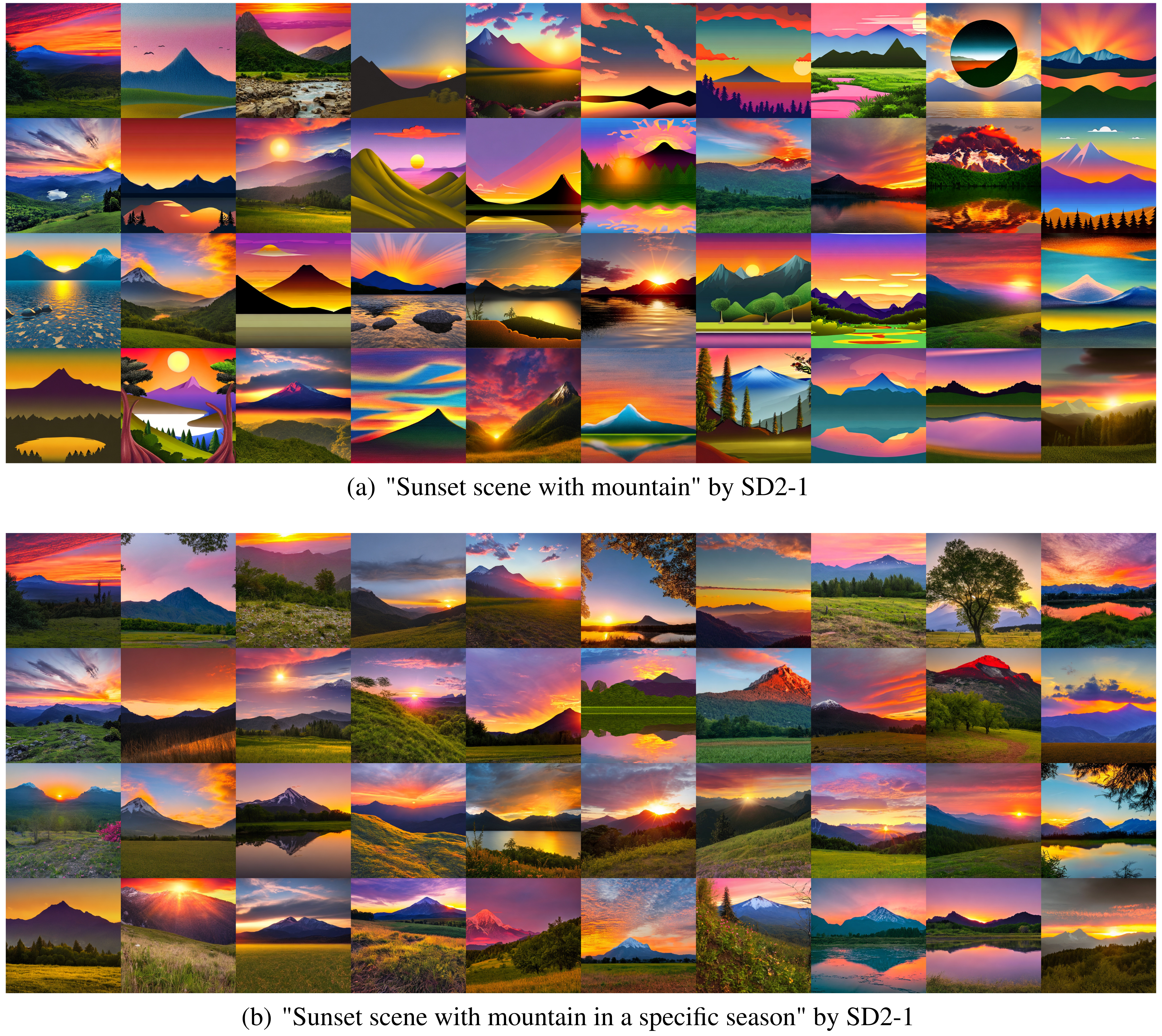
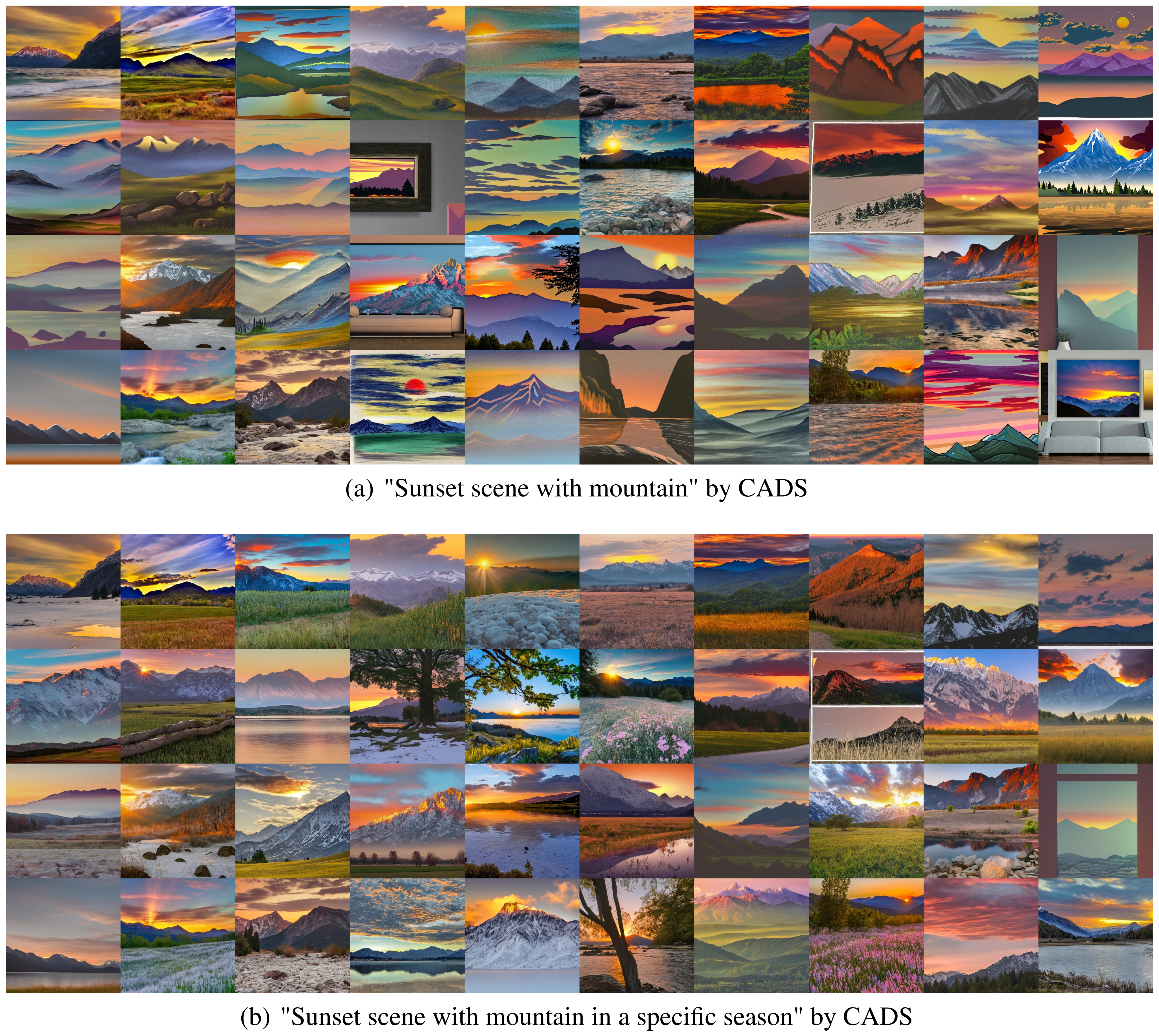
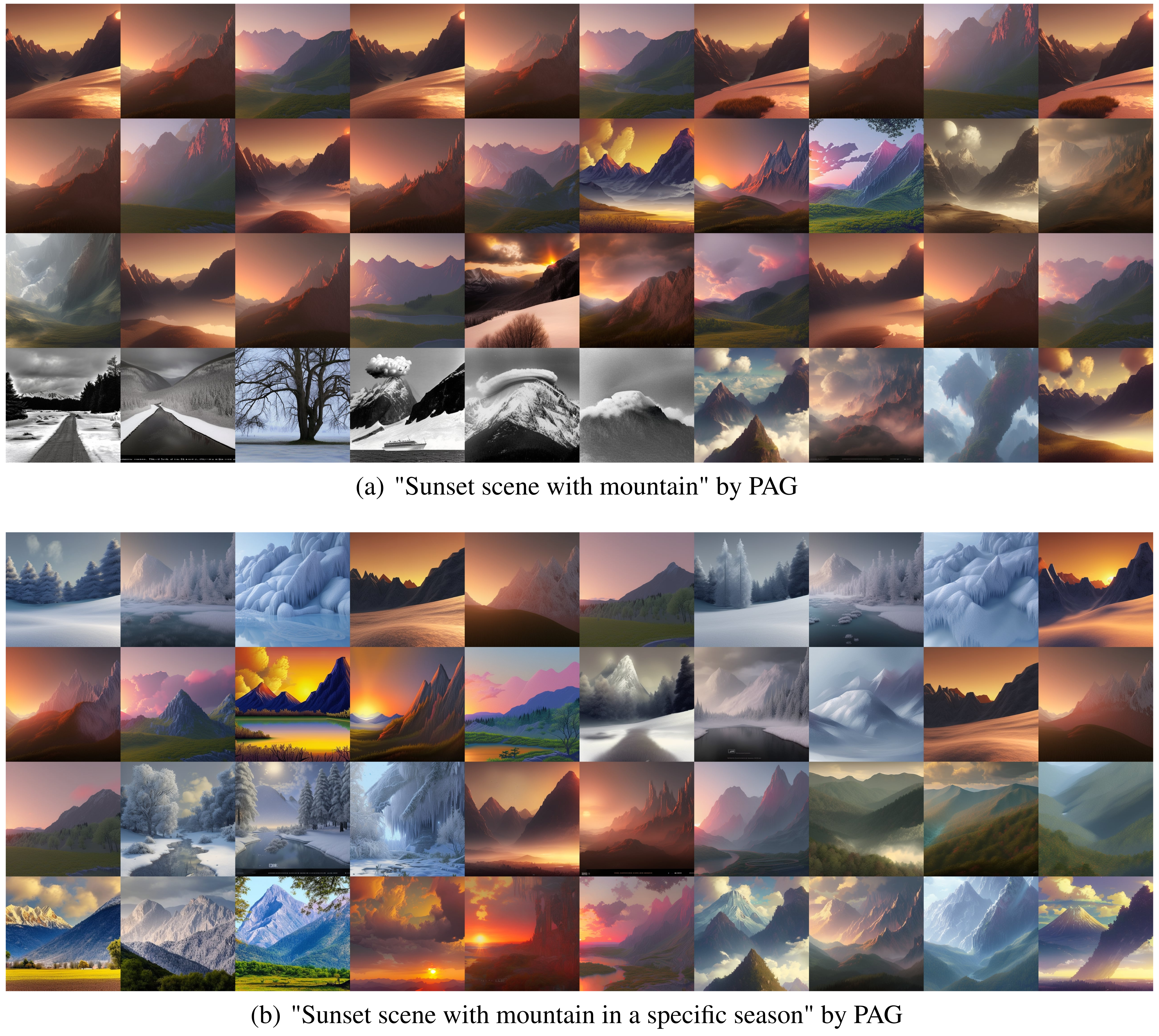
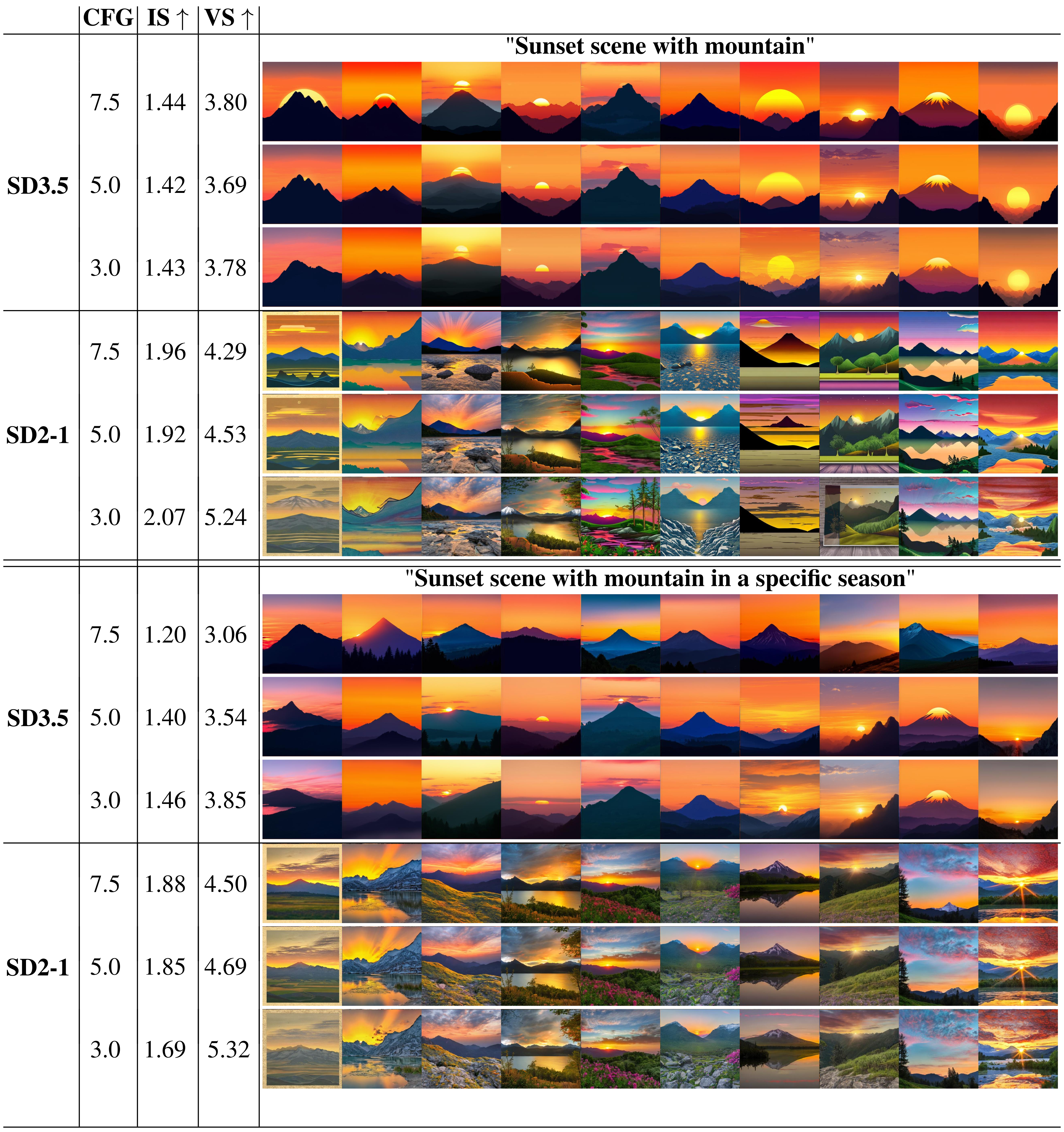
Figures 12–17 retain the 40-sample sunset galleries and all four seasonal edge interventions; Figure 19 retains both complete editing grids. Figure 18 compares classifier-free guidance settings. Its broad claim that reducing guidance does not improve contextual diversity should be read narrowly: the displayed Vendi values rise for SD2-1 on both prompts as guidance falls, and also rise for the seasonal SD3 comparison. This small sweep does not establish a universal absence of a guidance/diversity tradeoff.
E.4 Addition prompts for Text-to-image task
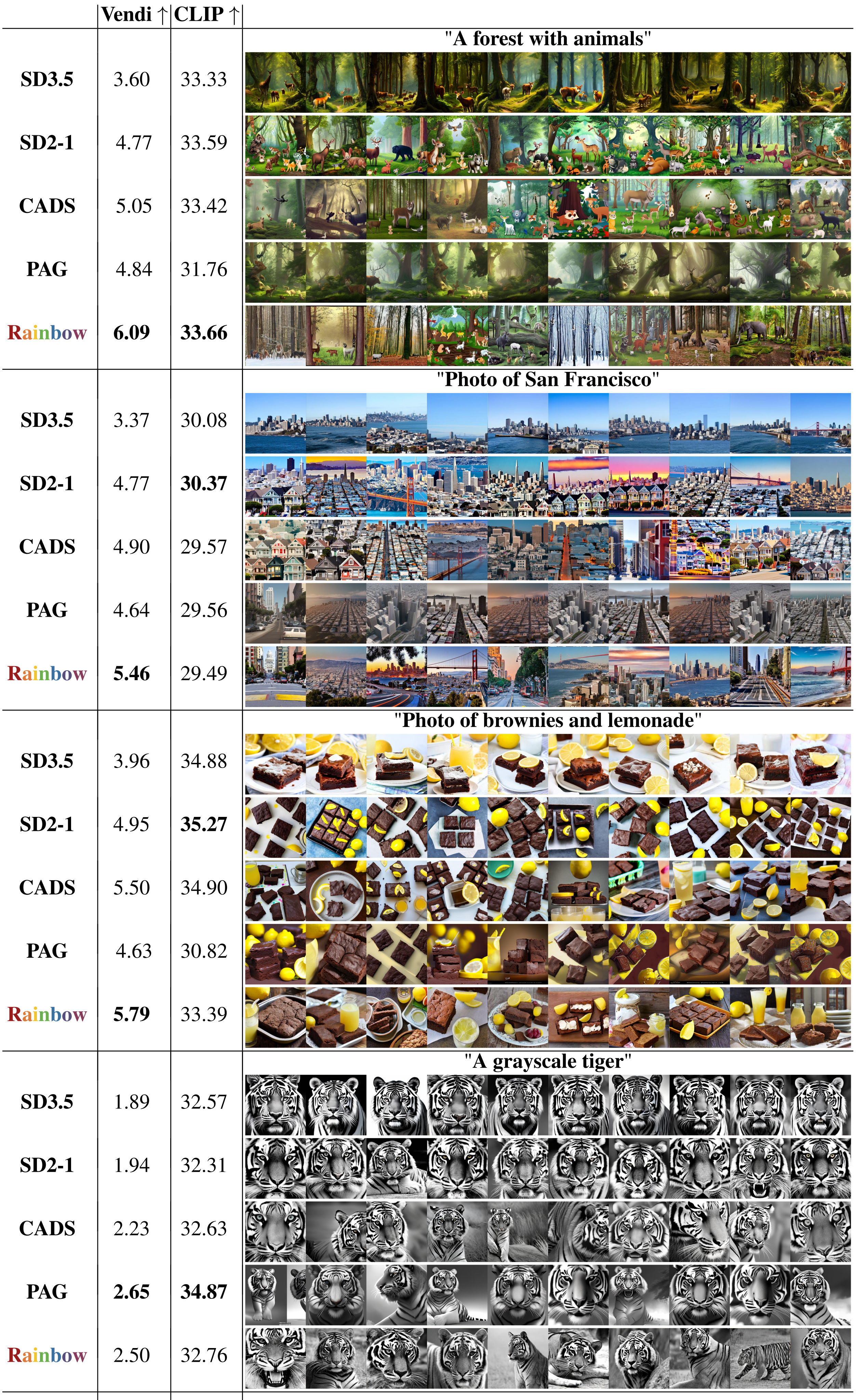
Figure 20 adds forest, San Francisco, brownies/lemonade and grayscale-tiger prompts. Rainbow has the highest Vendi on the first three, but PAG is higher for tiger (2.65 versus 2.50). CLIP can favor a baseline: SD2-1 scores 30.37 versus Rainbow 29.49 for San Francisco and 35.27 versus 33.39 for brownies/lemonade. Figure 21 preserves failure galleries, so the examples do not support a claim of uniform superiority.
E.5 3D Brain MRI Fidelity Analysis
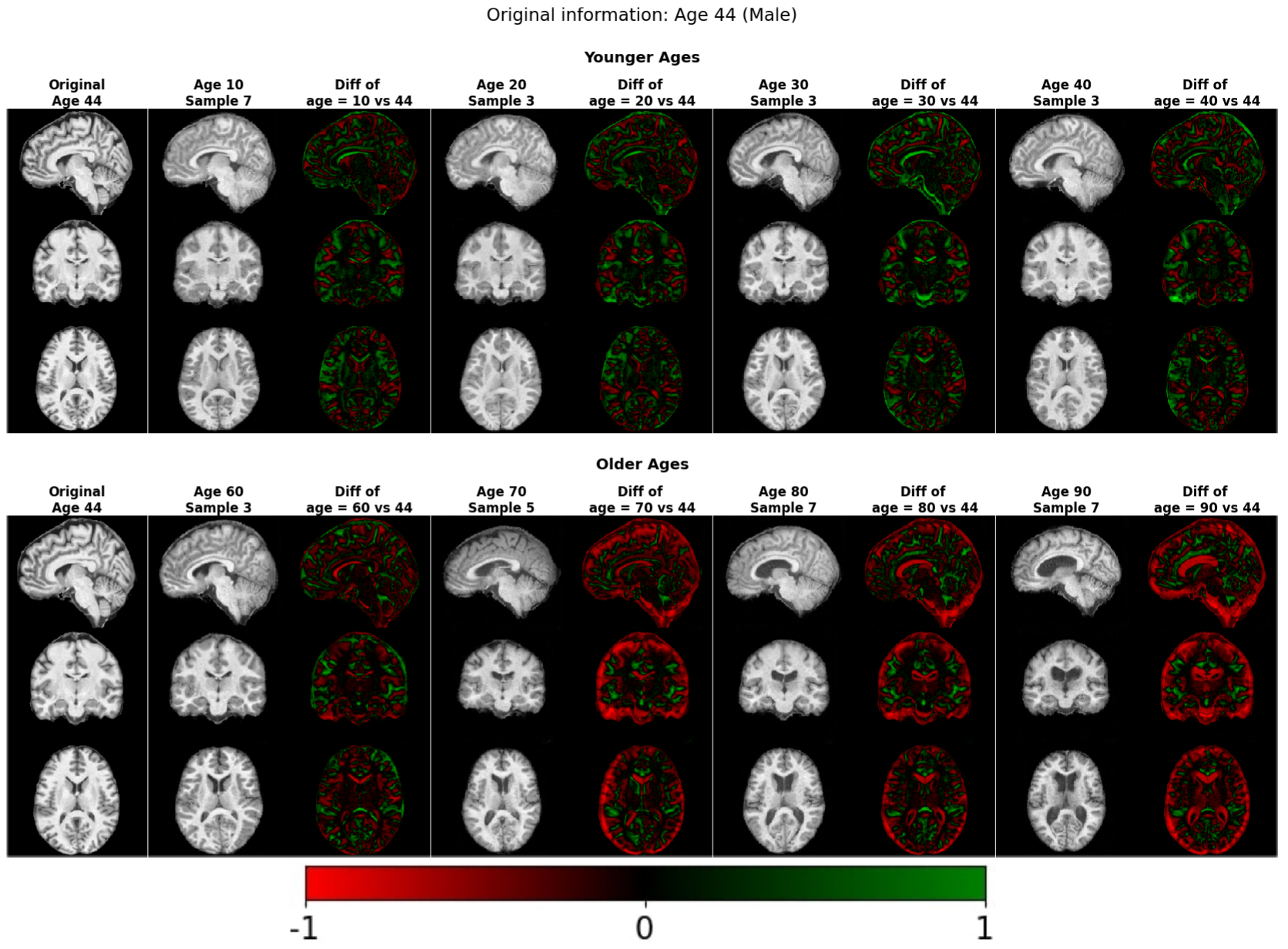
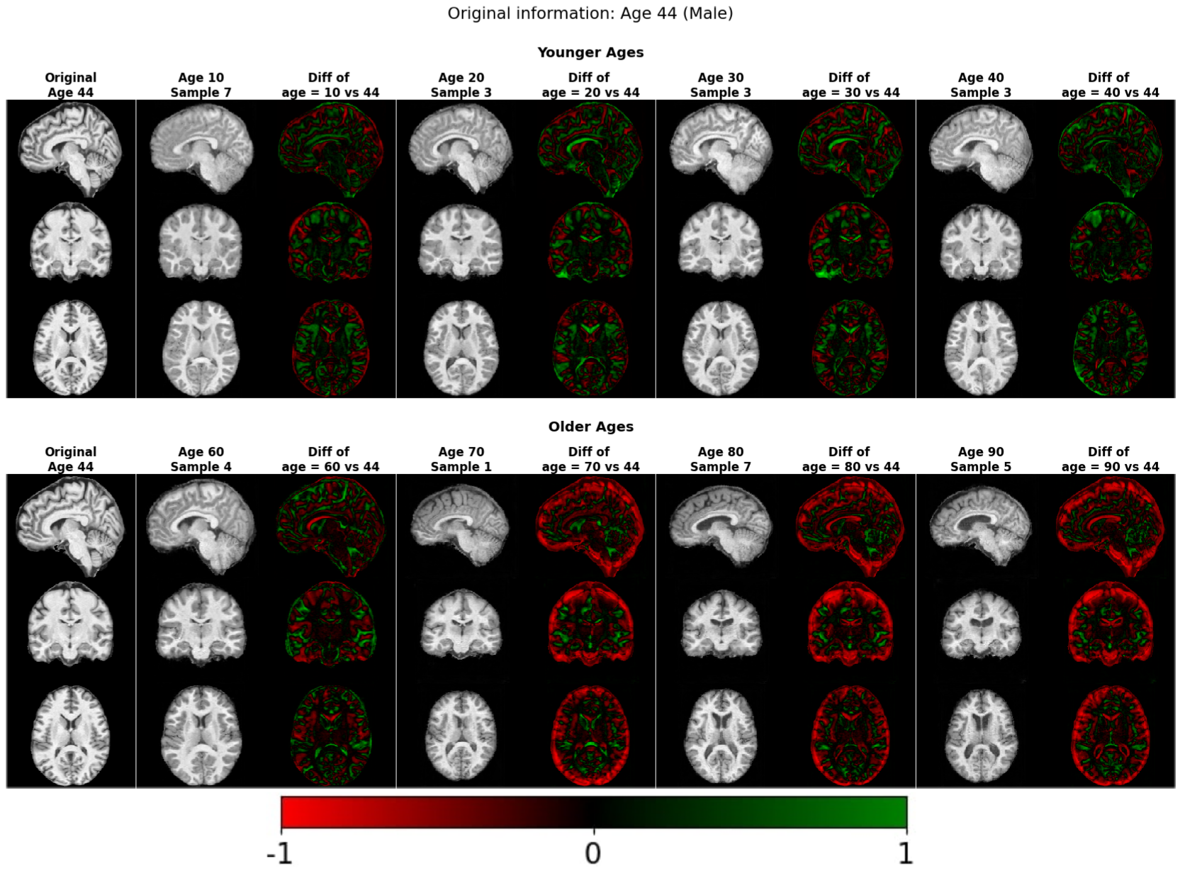
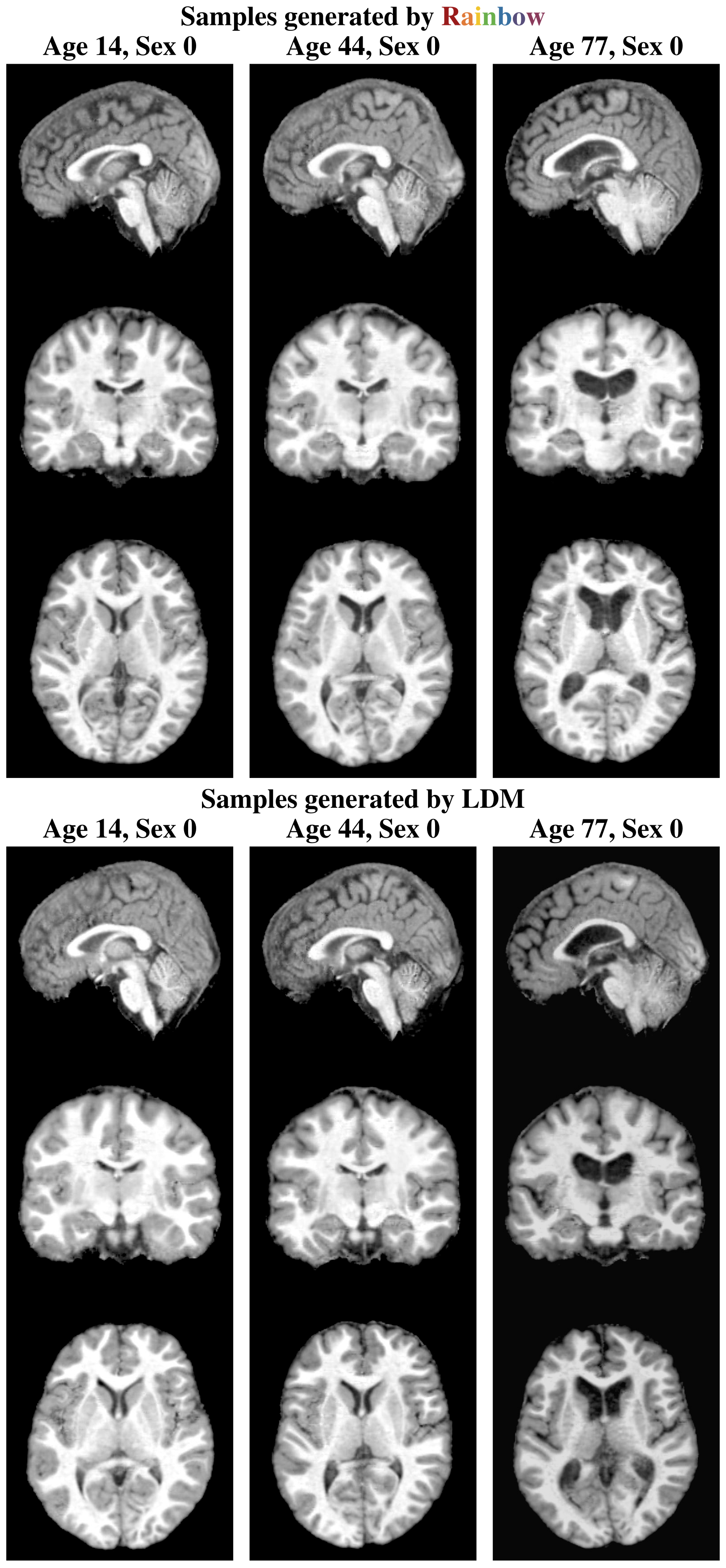
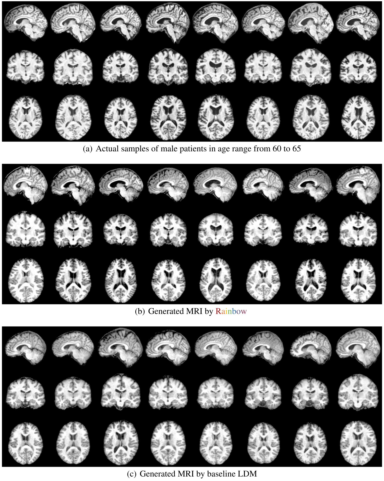
The MRI slices illustrate differences in apparent sharpness and anatomy, while X-ray grids and edge heatmaps show generated variation and prompt-linked edge frequencies. These remain visual demonstrations without an anatomical validity test. Appendix prose compares ages 14/16, 45/44 and 75/72, whereas Figure 27 labels both model rows 14, 44 and 77; the original figure is preserved. Likewise, the real comparison cohort is described as 63–65 in Figure 5 and 60–65 in Figure 28.
E.6 Qualitative Results for 3D MRI Counterfactual Generation Task
Figures 29–30 preserve age-edited MRI volumes and signed difference maps for Rainbow and LDM. The text additionally discusses binary-sex conversion and Table 1 reports its predictor metrics, but these two figures display age changes. The selected examples are consistent with the authors’ intended age effects; they do not verify longitudinal identity preservation, a causal age intervention, or clinical plausibility for each generated anatomy.