Overview
The reviewed arXiv v2 is dated 4 March 2026 and marked as an ICLR 2026 conference paper. Affiliations are MIT, UW–Madison and MIT-IBM Watson AI Lab; Xinyi Gu’s work was conducted during an internship at the lab. All six appendices are retained.
At a glance
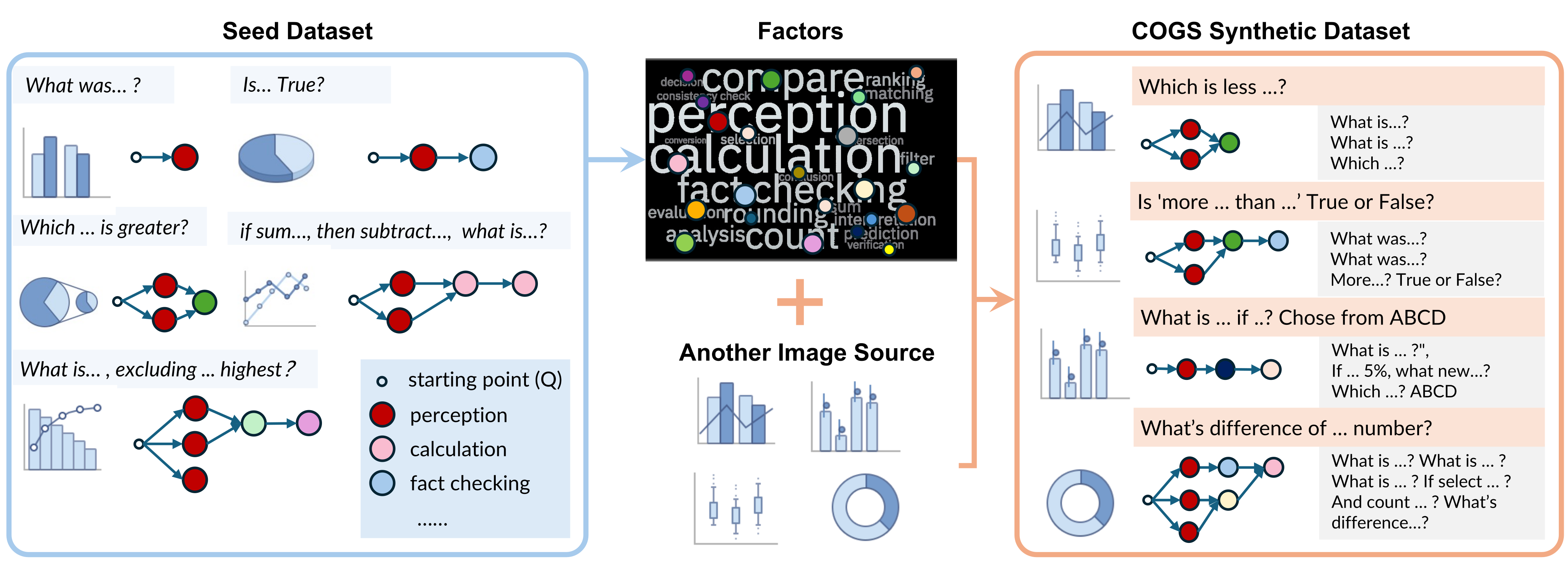
COGS decomposes seed visual questions into perception and reasoning factors, then recombines those factors on new images to create synthetic question–answer data. Each generated example includes intermediate subquestions and answers that can shape reinforcement-learning rewards.
Fine-tuning improves the evaluated chart and webpage question-answering models. ChartQAPro accuracy rises 47.36→52.02 and VisualWebBench 85.65→88.04 for Qwen2.5-VL-7B. The evidence concerns held-out questions from these benchmarks, not demonstrated document editing or web-agent execution. Project resources accompany the paper.
1 Introduction
Charts and webpages are abundant, but human-written questions requiring several reasoning steps are scarcer. A small seed set can expose reusable operations such as reading values, comparing quantities and arithmetic.
COGS uses that factor structure to synthesize new questions on separate image sources, then trains a pretrained multimodal model with final-answer and intermediate-answer feedback. This targets question diversity and supervision quality; it still relies on a strong pretrained generator and substantial fine-tuning computation.
2 Related Work
Prior instruction-synthesis methods such as Self-Instruct expand text prompts or evolve their complexity. COGS instead grounds reusable subquestions in visual inputs. Chart-specialist systems either extract structured data for an LLM or learn perception/reasoning jointly.
GUI research spans page question answering, element localization and agent behavior. This work evaluates screenshot question answering. Its learned factors are induced with a pretrained MLLM and supplied examples, so they are not independent of model priors or prompting choices.
3 COGS
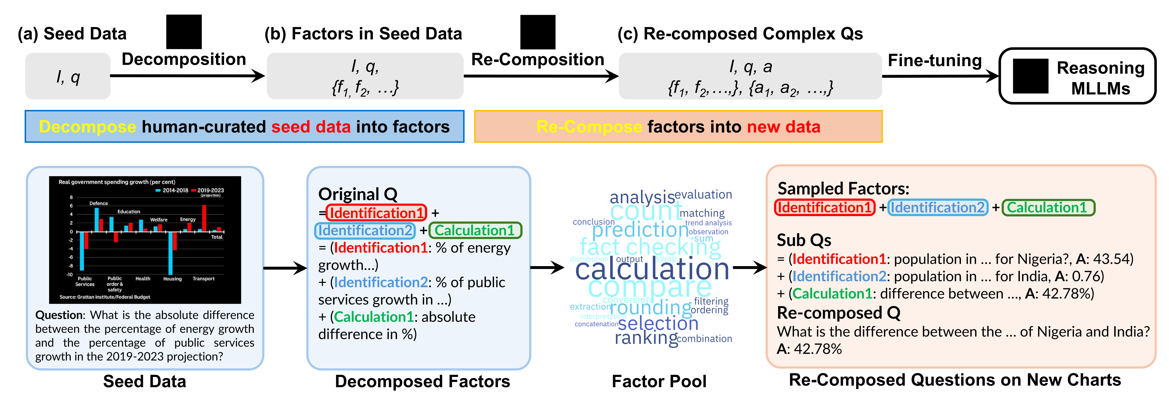
The pipeline decomposes seed questions, builds a pool of factor categories with exemplar subquestions, recomposes sampled factors on new images, and fine-tunes an MLLM using the resulting questions and intermediate answers.
3.1 Problem Formulation
A question is represented as ; factors include perception, arithmetic, logic and spatial relations. A small seed question set defines the domain’s candidate factor pool.
Seed answers are not required. Seed questions and associated images still provide domain supervision, and a pretrained generator supplies synthetic answers. The aim is novel valid compositions, not arbitrary generation disconnected from the image.
3.2 Seed Data Decomposition
A prompted MLLM receives the seed image, question, task instructions and in-context examples. It outputs category labels and grounded subquestions: for example, identify two growth percentages and compute their absolute difference.
Aggregation groups exemplar subquestions by categories such as calculation, counting and comparison. These examples guide later synthesis, while the generated decomposition supplies process-reward targets. The paper does not quantify a human-verified decomposition error rate.
3.3 Question Generation via Factor Recomposition
For a new image, the generator receives sampled factor categories and exemplar subquestions. It creates grounded subquestions, answers them, and composes an overall question and final answer. The resulting tuple is , with .
Available underlying chart metadata helps improve answer precision. Thus the method does not require new human QA labels, but some synthesis benefits from structured image metadata. Generator-produced answers are supervision targets rather than independently guaranteed ground truth.
3.4 Reinforcement Learning-Based Fine-tuning
GRPO fine-tunes the model. An LLM-based reward model checks whether its reasoning contains each generated sub-answer, producing a mean subquestion hit rate. StandardRM rewards final correctness; ProcessRM-sum adds weighted intermediate accuracy; ProcessRM-max takes the larger of the final and weighted intermediate rewards. Original definitions, proposition and proof expressions remain below.
For a binary final reward and 0<λ<1, a correct output receives max reward one; an incorrect output may receive partial shaping reward. This avoids rewarding a correct answer above one just because it matches a particular decomposition.
The claimed policy-order guarantee requires an extra restriction: the proof uses the same conditional error mean c on failed outputs across policies, although the proposition does not state that invariance. If failure rewards differ, order can reverse. For example, with λ=0.5, final accuracy 0.6 and zero failure shaping yields reward 0.6, whereas accuracy 0.5 with failure shaping one yields 0.75. The original stated assumptions allow this case.
The displayed affine relation is valid with a policy-independent c, not a general guarantee under arbitrary noisy process rewards. Likewise, the footnote’s “if and only if” condition for continuous final rewards is not established generally. The empirical reward ablation remains evidence for this training configuration.
Equations
Formally, let denote the correctness of the final answer for output , the number of subquestions, and a weighting hyperparameter. We define the subquestion hit rate as In this work, we consider three reward models:
- •
StandardRM: which only evaluates final-answer correctness. This is the default option when subquestion supervision is not available.
- •
ProcessRM-sum: which combines correctness of the final answer with the average subquestion accuracy, encouraging faithful reasoning at the factor level.
- •
ProcessRM-max: which prioritizes the final answer but still provides reward shaping when the intermediate reasoning is largely correct.
Proposition 3.1
Assume ** * When takes values from , ProcessRM-max preserves policy orders iff. ., and . is a noisy shaping reward: and with . Note that may vary with . Define
- •
ProcessRM-max preserves policy orders. For any policies ,
- •
ProcessRM-sum does not necessarily preserve policy orders. That is, there exist policies with ,
Proof sketch. Using , . With and , we get , which is an affine, strictly increasing transform of if .
4 Experiment
Evaluation covers ChartQAPro, MMC-Bench and VisualWebBench, with additional reward, seed-size and backbone ablations. The primary base model is Qwen2.5-VL-7B.
| Model | Factoid | MCQ | Convers. | FactChk. | Hypoth. | Overall |
| Proprietary Models | ||||||
| GPT-5-nano | 45.95 | 63.64 | 49.40 | 63.58 | 49.82 | 50.74 |
| GPT-4o-mini | 43.63 | 66.43 | 45.48 | 59.88 | 45.20 | 48.32 |
| Gemini 2.5 Flash-Lite | 40.42 | 19.96 | 48.77 | 37.43 | 16.66 | 38.72 |
| Claude Haiku 3.5 | 43.44 | 65.03 | 39.84 | 61.79 | 38.77 | 46.74 |
| Opensource Models (7B+) | ||||||
| Qwen2.5-VL-7B (base) | 42.07 | 62.59 | 44.88 | 60.78 | 50.72 | 47.36 |
| InternVL3.5-GPT-OSS | 43.02 | 58.74 | 42.86 | 58.02 | 54.48 | 46.86 |
| Phi-4-14B | 23.18 | 34.27 | 40.93 | 46.91 | 36.31 | 31.61 |
| Chart Specialist Models | ||||||
| ChartLLaMA | 8.11 | 23.08 | 18.37 | 45.06 | 29.55 | 17.19 |
| ChartMoE | 19.03 | 35.66 | 32.97 | 45.68 | 27.08 | 27.28 |
| Prompting Strategies: over Qwen2.5-VL-7B | ||||||
| Self-Consistency | 43.44 | 61.54 | 44.00 | 59.82 | 41.76 | 47.22 |
| Tree of Thoughts | 40.01 | 57.94 | 41.55 | 54.13 | 53.35 | 44.44 |
| Decompositional CoT | 42.08 | 65.03 | 42.57 | 56.53 | 45.55 | 46.36 |
| Data Synthesis Approaches: over Qwen2.5-VL-7B | ||||||
| ChartQA-Train | 38.77 | 60.14 | 49.72 | 61.11 | 53.12 | 46.64 |
| Chart-R1 | 42.17 | 46.85 | 50.53 | 61.11 | 55.55 | 47.32 |
| In-Context Q Example | 46.33 | 62.94 | 46.91 | 61.11 | 61.72 | 50.58 |
| COGS (Ours) | 46.88 | 65.73 | 51.16 | 61.85 | 58.25 | 52.02 |
4.1 Chart Understanding
Chart experiments test both transfer from a seed subset to held-out questions and mixing factors from two chart benchmarks.
4.1.1 Generalization From Seed to Target Dataset
ChartQAPro has 1,948 human-curated QA pairs. The authors use 33% of its released test set as seed/validation questions and hold out 67% for evaluation. Synthetic training images come from the separate ChartQA training set. These scores therefore use the paper’s custom split, not the full untouched benchmark test set.
Data-synthesis baselines use the same base model, image source and stated training effort. They use final-answer-only StandardRM because they lack subanswers; full COGS also changes reward supervision. Proprietary/open models, chart specialists and inference-time prompting provide additional comparisons.
COGS reaches 52.02 overall versus base 47.36 (+4.66 points), in-context-example synthesis 50.58 and GPT-5-nano 50.74. It is best overall in the listed chart table, not on every question type: the in-context baseline has higher hypothetical accuracy, and some proprietary models lead MCQ or fact checking.
The text’s claim that all synthesis methods help is too broad: ChartQA-Train scores 46.64 and Chart-R1 47.32, both below the 47.36 base. Explanations involving domain gaps and reduced error accumulation are plausible interpretations rather than isolated causal measurements.
4.1.2 Generalization over Mixture of Datasets
MMC-Bench is split 33% seed/67% evaluation. Data-level mixing synthesizes separately and combines examples; factor-level mixing merges factor pools before synthesis. Both use ProcessRM-max. The original composition formulas are retained below.
Factor mixing beats data mixing on ChartQAPro (52.33 versus 50.72) and MMC (87.55 versus 86.99). It slightly exceeds ChartQAPro-only training on that benchmark (52.02), but remains below MMC-only training on MMC (88.10). Single-domain models are reference points, not mathematical upper bounds.
The results support useful transfer in these splits; they do not establish universal absence of dataset-specific overfitting. ChartQAPro-only training scarcely changes MMC (85.65→85.69), so cross-domain gains are not uniformly substantial.
| Model | ChartQAPro | MMC |
| Qwen2.5VL | 47.36 | 85.65 |
| + ChartQAPro | 52.02 | 85.69 |
| + MMC | 49.93 | 88.10 |
| + Data-level Mix | 50.72 | 86.99 |
| + Factor-level Mix | 52.33 | 87.55 |
Equations
Data-level mixture
Factor-level mixture
4.2 Webpage GUI Understanding
VisualWebBench supplies seed questions and held-out evaluation, while MultiUI supplies new screenshots. The comparison also fine-tunes on ten thousand sampled MultiUI webpage QA examples.
COGS reaches 88.04 versus base 85.65, inference-time decomposition 86.12 and MultiUI-WQA 86.60. It is the best listed nonproprietary model; GPT-5-nano scores 89.47. This shows transfer of the synthesis recipe to webpage QA, not downstream browser-action capability.
| Model | WebQA |
| Proprietary Models | |
| GPT-5-nano | 89.47 |
| GPT-4o-mini | 81.34 |
| Gemini 2.5 Flash-Lite | 81.85 |
| Claude Haiku 3.5 | 80.86 |
| Opensource Models (7B) | |
| Qwen2.5-VL-7B (base model) | 85.65 |
| InternVL3.5-GPT-OSS | 74.64 |
| Phi-4-14B | 74.16 |
| Specialist Models | |
| UiX-Qwen2 | 68.90 |
| Inference-time decomposition | |
| Decompositional CoT | 86.12 |
| Data Synthesis Approaches | |
| MultiUI-WQA | 86.60 |
| COGS (Ours) | 88.04 |
4.3 Additional Analysis
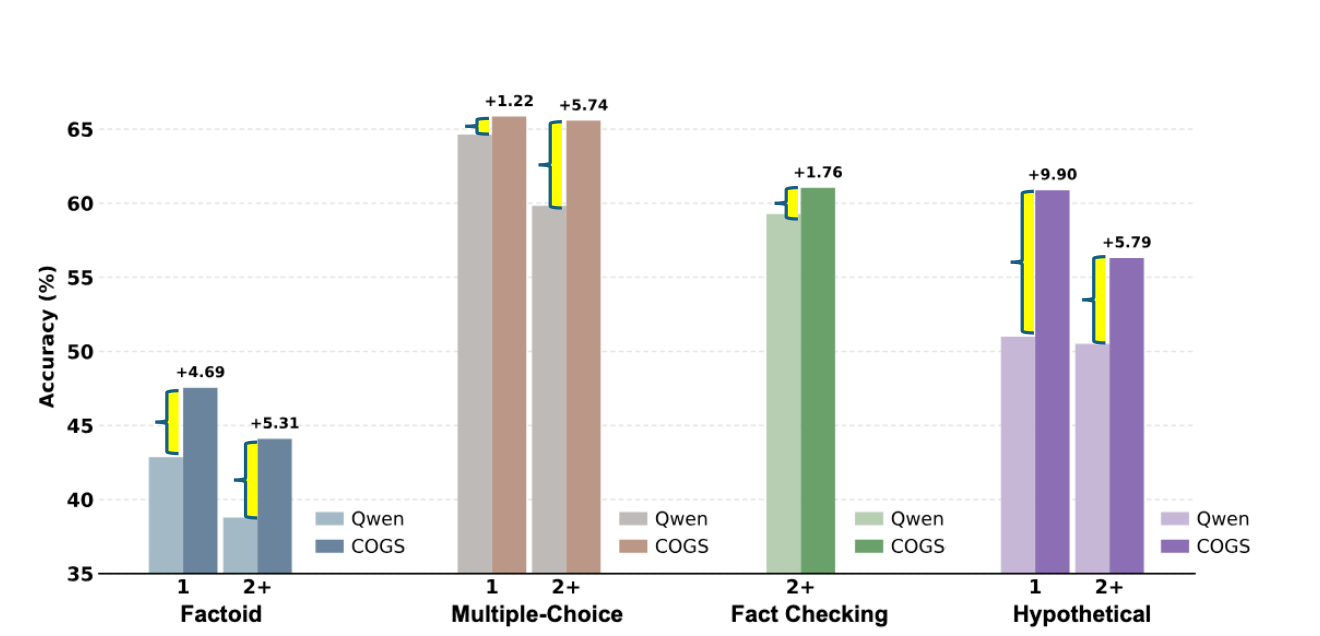
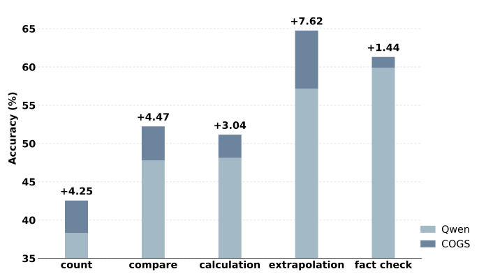
Factor-stratified plots show larger gains on many longer reasoning chains, especially factoid, multiple-choice and fact-checking questions. Hypothetical questions show a weaker pattern. Gains by factor include counting +4.25 points, comparison +4.47, calculation +3.04, extrapolation +7.62 and fact checking +1.44.
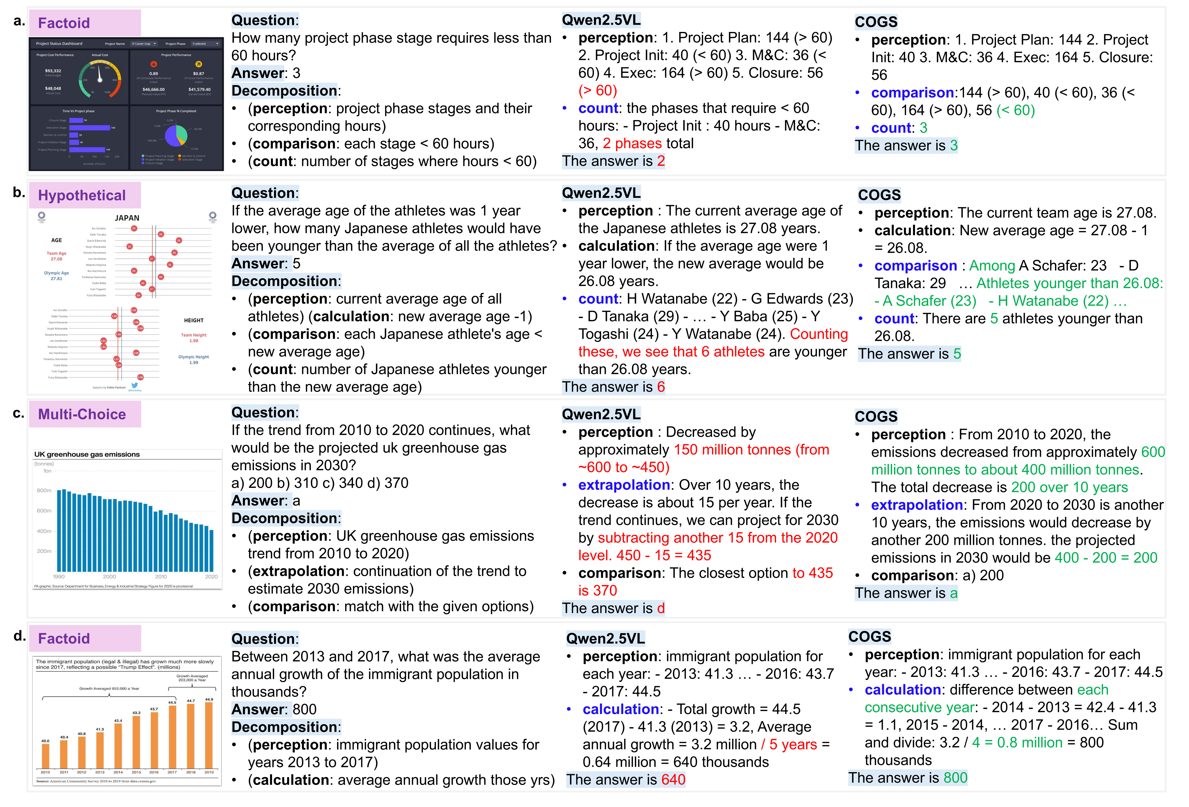
Figure 5 retains four selected examples: threshold counting, a counterfactual age comparison, trend extrapolation and average growth over four intervals rather than five years. These illustrate successful corrections, without independently measuring general chain-of-thought faithfulness.
With the same COGS data, StandardRM scores 50.96, ProcessRM-sum 50.35 and ProcessRM-max 52.02. Thus max shaping adds 1.06 points over final-only reward in this experiment. Prepending SFT on a separate 35k-example set reduces the final score to 46.62 despite improving output format; disjoint SFT/GRPO examples do not guarantee better reasoning.
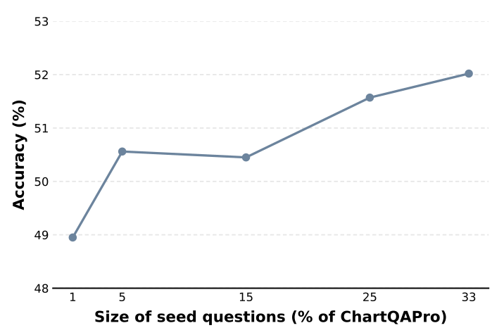
Seed-size ablations hold the 67% evaluation split fixed and use 1%, 5%, 15%, 25% or 33% of the original dataset as seeds. Performance broadly rises with seed coverage, with a small early nonmonotonicity in the plotted curve. No repeated-seed error bars or statistical-significance tests are reported.
| Reward Model | Overall Acc. |
| StandardRM | 50.96 |
| ProcessRM-sum | 50.35 |
| ProcessRM-max | 52.02 |
| Alt. Training Setting | |
| SFT+ProcessRM-max | 46.62 |
5 Conclusion
COGS uses factor recomposition to turn a limited set of visual questions into richer synthetic supervision. The experiments support improvements in chart and webpage QA, including benefits from mixing factor pools and using max-style process rewards.
Long documents, integration into pretraining, search-based reward guidance, chart-code editing and web-agent tasks are future directions. “Data-efficient” refers to human seed questions, not demonstrated low total GPU or generation cost.
Ethics Statement
The authors state that source data are publicly released, used under their licenses, and that synthesis stays within chart/webpage reasoning without generating images. They aim to avoid offensive or sensitive content. These are the paper’s stated practices; no independent bias or safety audit is reported.
Reproducibility Statement
The paper points to public model weights/APIs, released code/data and the prompts and settings in Appendix D. The retained appendix gives the reported versions and compute configuration; it does not fully specify every reward-judge setting or λ value.
Acknowledgments
The authors thank Lei Xu, Bowen Pan, Pingchuan Ma and MIT-IBM Watson AI Lab colleagues for discussion and feedback.
Appendix
The appendices document language-model use, webpage examples, backbone ablations, implementation settings, complete prompts and synthesized examples.
Appendix A The Use of Large Language Models (LLMs)
ChatGPT was used for grammar checking. Small proprietary models serve as evaluation baselines, and an open-source MLLM generates synthetic data under its license.
Appendix B Qualitative Evaluation on VisualWebBench
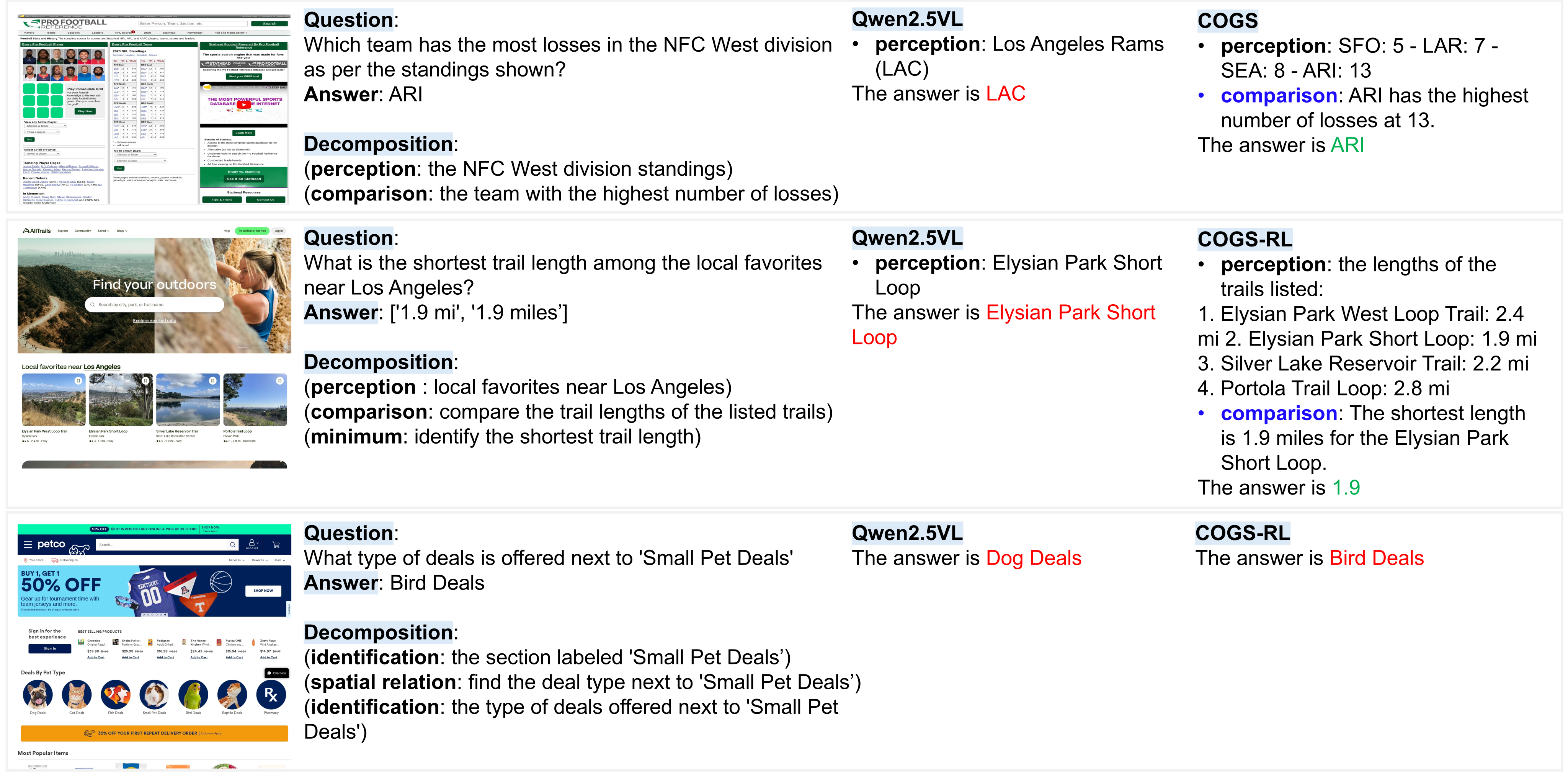
Figure 7 preserves three webpage examples involving sports standings, trail-length comparison and neighboring deal categories. The examples demonstrate selected successful reasoning/spatial corrections, rather than a representative error taxonomy.
Appendix C Ablation Study on Base Models
Under the reported same data and RL configuration, Qwen2.5-VL-3B improves 36.22→38.68 and LLaVA-v1.5-7B 13.47→22.04 on ChartQAPro. Gains occur across these two additional backbones, although their final accuracies remain below the main 7B model.
Appendix D More Details about COGS Implementation and Reproducibility
Implementation details cover distributed training, synthetic-data generation, runtime and evaluation prompts.
Hyper-parameters
Training uses VERL for four epochs with batch 1,024, minibatch 256, learning rate 10⁻⁶, prompt/response limits 4,096/2,048 tokens and sixteen rollout samples per step. A 0.001 KL penalty is included in the loss while KL reward is disabled. Gradient checkpointing, tensor parallel size two and 0.6 GPU-memory utilization are reported.
Running Software/Hardware Environment and Training Time
The environment uses Transformers 4.51.3, PyTorch 2.6.0, CUDA 12.4 and VERL 0.5.0.dev0 on four nodes with eight 80-GB H100s each. Qwen2.5-VL-72B generates training data.
For ten thousand reasoning examples, chart GRPO takes about ten hours and webpage GRPO twenty-one hours; chart SFT is reported as two hours. The larger webpage screenshots increase cost. Generation and reward-judge compute are not separately quantified, and the text does not reconcile the timing example’s data count with the separate 35k SFT ablation.
Evaluation
Evaluation uses each benchmark’s held-out 67%, official chain-of-thought category prompts for chart QA, and lmms-eval. The webpage instruction requires step-by-step reasoning followed by “The answer is X” with a concise final answer. The complete original instruction is retained below.
You will be given an image and a question that you need to answer based on the provided image. You need to think step-by-step and format the final answer in a separate sentence like “The answer is X”. The final answer should be in the fewest words possible.
Prompt for Seed Question Decomposition and New Question Recomposition are included in the next section.
Appendix E retains the exact decomposition and recomposition prompt templates.
Appendix E Prompts
All prompt text and embedded output-format examples are preserved below. These are model instructions used in the method.
E.1 Prompts for Question Decomposition
The decomposition prompt requests image-grounded factors in the example format, omits answers, and avoids unnecessary decomposition for simple identification. Four chart examples illustrate count/comparison, trend fact checking, percentage arithmetic and a counterfactual premium calculation.
The block labeled for webpage GUI decomposition still contains chart-style examples in the published source. That mismatch is retained rather than silently replacing the examples.
We can decompose each question into subquestions from one of the general types. Here are some examples:

[in-context example: Chart/Web] Please do the same for the following questions in the same format without explanation.

Check the information in the attached image carefully. If the question can be easily answered with a simple identification step, avoid unnecessary decomposition.

Remember to strictly follow the format of the example, and don’t provide the answer. <image> Question: {query}
(Question: How many times has the satisfied rate been above 25%?) = (identification: satisfied rate of each year) + (comparison: each instance > 25 % ) + (count: number of instances where satisfied rate > 25 % ) (Question: Is the following statement True or False? Gen X has experienced a steeper population increase than baby boomers did between 1990 and 2015.) = (identification: Gen X’s population increase curve) + (identification: baby boomers’ increase curve) + (comparison: which one has a steeper curve) + (fact checking: given the finding from the previous step, is the statement true?) (Question: if a multi-college district served 10,000 students, how many students were determined eligible using EFC criteria?) = (identification: percentage of students determined eligible using EFC criteria in a multi-college district) + (calculation: number of students based on that percentage) (Question: if the actual Avg ACA Premium in 2017 had turned out to be $5,000, and the +30% label accurately reflected the difference compared to the Low Est. projection for that hypothetical $5,000 value, what would be the implied Avg Individual Mrkt Premium Without ACA - Low Est. - in 2017?) = (identification: Avg ACA Premium in 2017) + (identification: +30% label that reflects the difference of Avg ACA Premium in 2017 compared to Low Est.) + (calculation: implied Low Est. value based on the given 30% difference and hypothetical $5,000 ACA Premium)
(Question: How many times has the satisfied rate been above 25%?) = (identification: satisfied rate of each year) + (comparison: each instance > 25 % ) + (count: number of instances where satisfied rate > 25 % )

(Question: Is the following statement yes or no? Gen X has experienced a steeper population increase than baby boomers did between 1990 and 2015.) = (identification: Gen X’s population increase curve) + (identification: baby boomers’ increase curve) + (comparison: which one has a steeper curve) + (fact checking: given the finding from the previous step, decide yes or no)

(Question: According to this chart, what is the revenue of Retailer D at Month 6?) = (identification: revenue of Retailer D at Month 6)
E.2 Prompts for Question Re-composition
Recomposition asks for exactly five unique grounded QA pairs using specified counts/types of factors. Later reasoning must depend on earlier identified values, and the concise question must remain independently understandable. The generator provides both reasoning and a short final answer.
The retained examples distinguish dependent reasoning from unrelated calculations and explain how to preserve counterfactual conditions when shortening a question. The two original JSON-like format/example listings retain their indentation, numeric keys and ellipses; they are prompt templates, not strict executable JSON.
Given the following chart:

chart: <image>

Your Task is to generate 5 sets of question-answer pairs for instruction tuning. In each set of QA pairs, you need to first identify {perception_count} entities, and then compose {reasoning_count} level of reasoning questions related to them. The 2-nd order reasoning questions should be based on the answers of the 1-st order reasoning questions, and so on. Each question must meet ALL these conditions:

1. Content Source: Only use data present in the given chart.

2. Structure: Each question must include exactly {count1} {factor1} , … , and {countN} {factorN} . Each identification question should ask about one and only one entity/concept, the following {reasoning_factors} subquestions should be the question related and only related to the entities/concept mentioned in the previous subquestions. The specific example of each subquestion type will be provided in the following text.

3. Content: Each question must be based on the chart data, and can be answered using natural language. Avoid asking about the size of an object that is not relevant to the data (e.g., font size of a label).

4. Relevance: If there is a reasoning subquestion, it must operate on the entities or values identified in the observation subquestion. [in-context example 1]

5. Conciseness: After writing the detailed question, provide a natural concise version. This concise version should still look like a question, and can be asked independently without the previous question. [in-context example 2]

6. Answer: Provide a step-by-step reasoning for how you found the answer.

7. Final Answer: Provide just the concise final answer to the concise question, without any explanation or reasoning.

Reference Examples: {factors} {sampled_subquestion_of_the_factor}

Here are some examples of the concise questions: {sampled_concise_questions} Expected Output Format for the generated questions: Use the following structure for each pair:

[in-context example 3] Instructions:

1. Follow the example strictly. If the question contains reasoning subquestions, make sure it is relevant to the observation questions.

2. Use only the given data in the chart.

3. Provide exactly 5 unique Q&A pairs. [question_types]

4. Validate each answer. The answer must be grounded to the data shown in the chart.

5. Each pair must include both detailed step-by-step reasoning and the final result. Generate Now:

Please proceed with generating your 5 question-answer pairs now.
For example, if the observation subquestion asked about the value of A and B, and you are asked to generate a calculation subquestion after them, it must be some calculation between A and B. If there are multiple levels of reasoning questions, the later reasoning subquestions should be based on the answers of the previous subquestions. Do not ask irrelevant questions. For example, if the first subquestion is “what’s the difference between A and B”, an acceptable next-level reasoning question would be “what’s the difference between A and B compared to C”. You should avoid an unacceptable question like “what’s the difference between A and B and what’s the difference between A and C”.
For example, if the detailed question asks about a new value if A is changed, the concise question cannot simply refer to a “new value” without mentioning it depends on A being changed. An explicit example: detailed question: “What is A, what is B, what is the new value of A+B if A is changed to 10, what is the difference between the new value and C?” A bad concise question is: “What is the difference between new value and C?”, because it does not mention A is changed to 10, and it does not mention A+B is the new value. A correct concise question should be: “What is the difference between the new value of A+B and C, if A is changed to 10?”
{
  1: {
    "Question": "<Full question with two identifications and one comparison>",
    "Concise question": "<Concise version of the question>",
    "Answer": "<Step-by-step reasoning and calculation>",
    "Final Answer": "<The final answer to the concise question>"
  },
  2: {
    "Question": "...",
    "Concise question": "...",
    "Answer": "...",
    "Final Answer": "..."
  },
  ...
}
Example (not actual data):
{
1: {
"Question": "What was the percentage for Technology, what was the percentage for Finance, and what is the difference between them?",
"Concise question": "What is the difference between Technology and Finance's percentages?",
"Answer": "Step 1: Technology's percentage is 23.7%. Step 2: Finance's percentage is 26.3%. Step 3: The difference is |23.7% - 26.3%| = 2.6%.",
"Final Answer": "2.6%"
}
}Appendix F COGS Data Example
The following figures retain complete synthesized questions, images, intermediate subquestions and answers.
F.1 Visualization of selected COGS-ChartQAPro
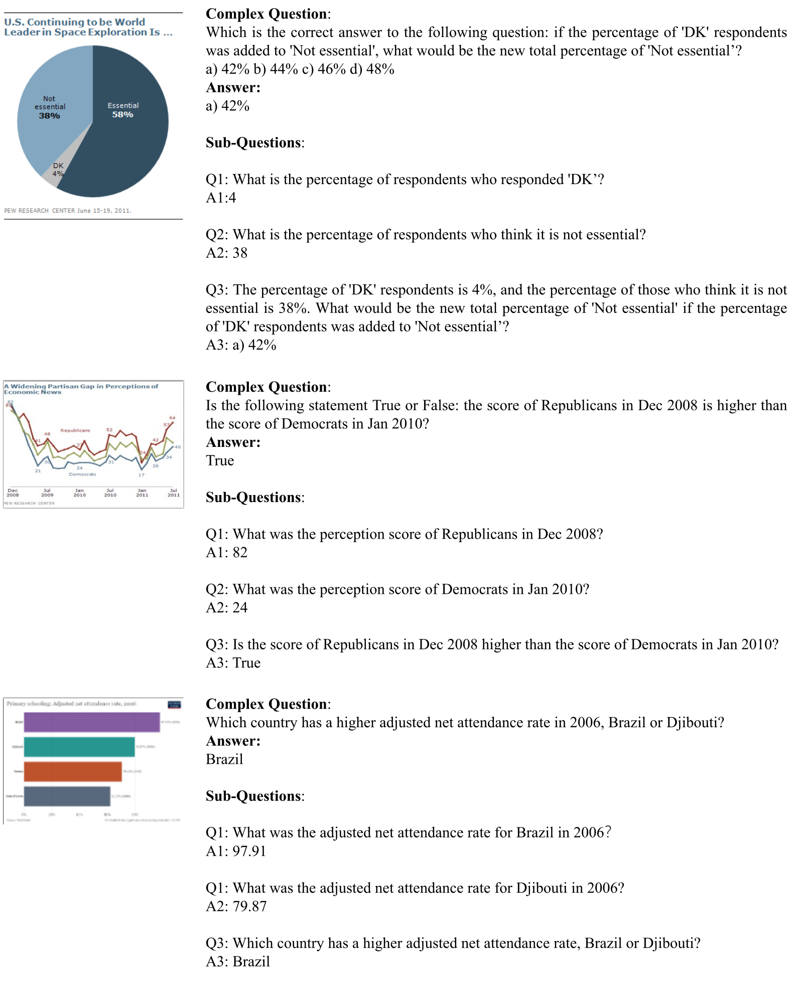
Figures 8–10 contain eight chart examples: three with three subquestions, three with four, and two with more than four. They include percentage addition, comparisons, counterfactual swapping/reduction, growth adjustments and nested differences.
Original labels and imperfect compositions remain visible, including repeated Q1 labels and an unused difference subquestion in the Google/Facebook example. These examples show why generated intermediate labels should be treated as potentially noisy supervision.
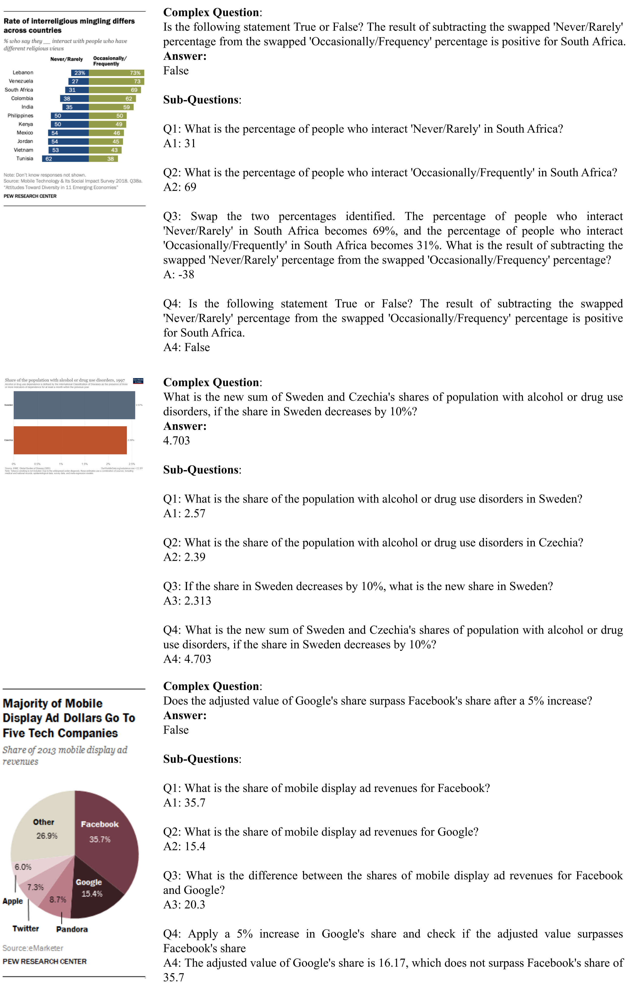
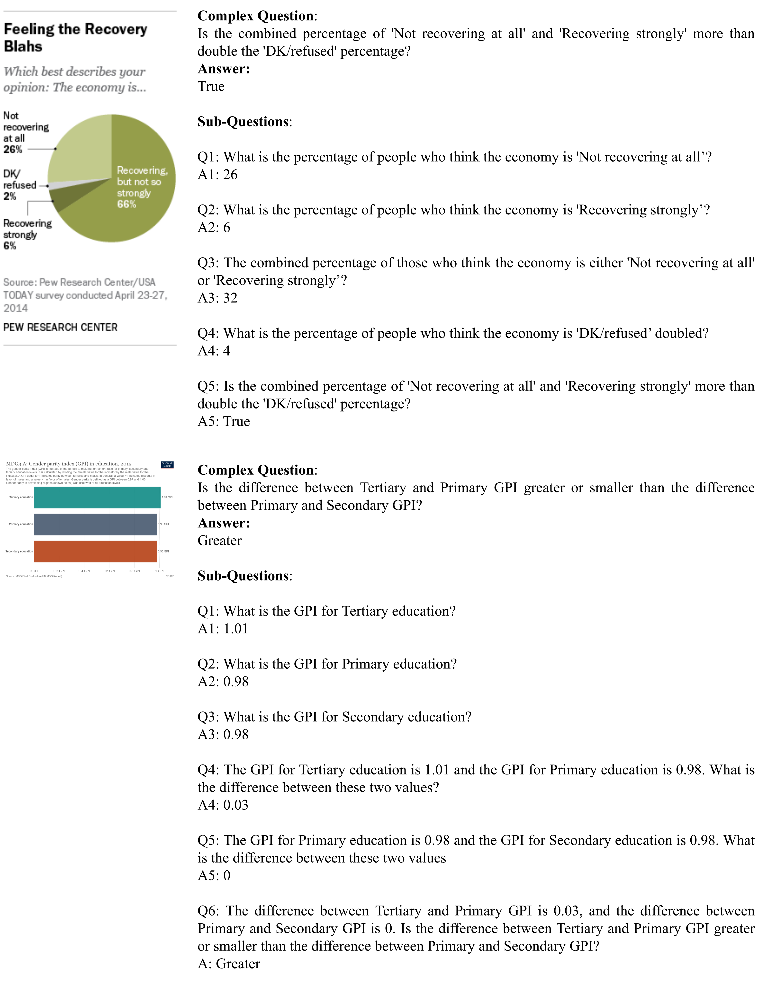
F.2 Visualization of selected COGS-VisualWebBench
Figure 11 retains three webpage examples: increasing a one-item hat order by two, extracting a postal code through the displayed city/address, and comparing publication years. All screenshot detail, questions and intermediate answers remain available; repeated source subquestion labels are unchanged.