At a glance
ConPoSe uses an LLM to propose contact points for several mobile robots pushing an object, then applies a small local search to improve the proposal. It avoids exhaustive enumeration of contact combinations and retains high selection-only success as the robot count grows to fifteen. The result is strongest when robot repositioning is automatic: real contact-switching behavior within the simulator causes large failures on the concave T-shaped object. Faster contact selection therefore does not by itself establish a reliable complete transportation system.
This edition follows the complete eight-page v1 manuscript dated October 9, 2025. It retains all four numbered figures and their panels, three tables, ten numbered equations, both complete algorithms and all 21 references. The numerical evaluation is in Webots; preliminary physical experiments mentioned in the conclusion are not documented as a separate benchmark. The stated complete online prompt has no link or text in this source.
I INTRODUCTION
Pushing lets simple robots move objects without grippers, but the contact locations determine the net force and rotation. As the object and robot team grow, enumerating all contact subsets becomes expensive. ConPoSe uses language-model reasoning as an initial proposal for a constrained search, while conventional planning and controllers perform the surrounding task.
The method knows the object footprint, its geometric center and the environment state. It assumes that the geometric center is the center of mass; it does not identify arbitrary mass distributions or learn friction. The contributions are a hybrid contact selector and simulation comparisons across shapes, scenes and team sizes, rather than a new perception or dynamics model.
II RELATED WORK
The relevant background concerns both cooperative pushing and the use of foundation models to propose geometrically meaningful robot configurations.
II-A Cooperative Object Pushing
Cooperative transport includes pushing, grasping and caging [1]. Prior pushing work varies in shape coverage, obstacle complexity and required physical information. Tang and colleagues use hierarchical hybrid search for multiple robots and complex scenes [5], but require more object information. ConPoSe borrows the contact-generation and assignment setting while substituting an LLM-guided search for exhaustive contact selection.
The round differential-drive robots create an additional difficulty: they cannot move sideways to preserve a desired contact. This nonholonomic contact problem is distinct from selecting a good ideal force configuration [12].
II-B Foundation Models in Robotics
Foundation models have been used for task planning, navigation, manipulation and multi-robot pattern formation [8][11]. PIVOT illustrates visual prompting for action proposals [14], while collaborative manipulation systems use vision-language reasoning [6]. ConPoSe itself sends a text description with numerical contact coordinates and directions, rather than asking a VLM to infer contacts directly from images.
Its task differs from static pattern formation because contacts must generate a target force direction and be changed repeatedly during execution. The paper claims novelty for foundation-model-guided collective pushing; the experiments compare the stated baselines, not every possible learned or optimization-based selector.
III PROBLEM FORMULATION
A homogeneous team of N round robots pushes an object along a preplanned two-dimensional waypoint path amid known static obstacles. Each candidate contact has a position and inward-normal pushing direction. The ideal model assigns equal force magnitude to every robot and sums those vectors; uniform mass makes the geometric center the center of mass.
Each configuration contains N distinct contacts. The objective is to reach the goal while staying near the object path and using few configuration changes, because moving robots around the object is costly. Unknown friction, slipping and imperfect contact maintenance violate the ideal force model, so geometric feasibility is not a guarantee of actual motion or collision-free execution.
Equations 1–5
| (1) |
| (2) |
| (3) |
| (4) | ||||
| (5) |
IV METHOD
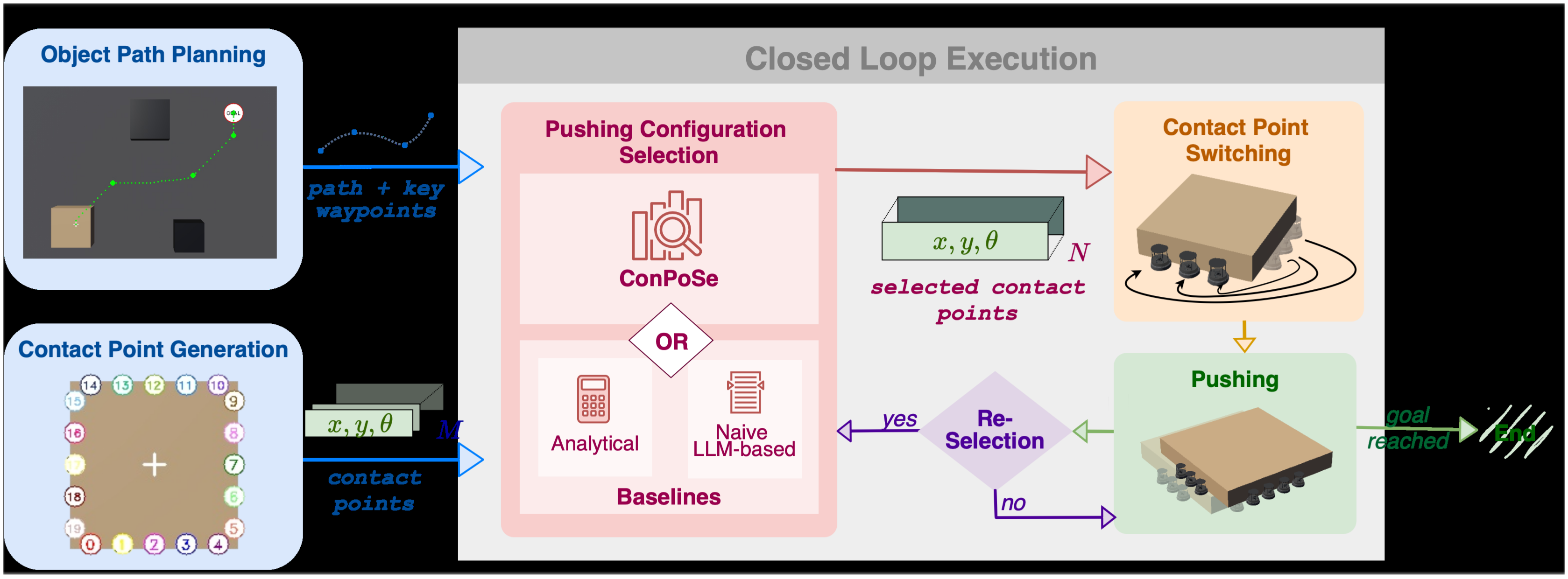
The full system plans an object path, discretizes the boundary, selects and assigns contacts, moves the robots to them, and pushes until the goal or a replanning condition is reached. The LLM is used at the contact-selection stage; the rest is explicit planning and control.
IV-A Object Path Planning
A* plans on an obstacle costmap with forbidden regions and a smooth clearance penalty extending to 1.5 times the safety radius. Ramer–Douglas–Peucker simplification extracts key waypoints and approximately constant-direction path segments. Equation 6 points from the current object center toward the next key waypoint.
The desired direction is recomputed from the actual object position. Planning uses known geometry; the manuscript does not provide a perception pipeline or a formal clearance guarantee under the unmodeled pushing dynamics.
Equation 6
| (6) |
IV-B Contact Point Generation
The object boundary is divided into segments at least as wide as a minimum spacing, adjusted for equidistant contacts along each edge. Additional margins protect concave corners. Short polygon edges approximating a circle are aggregated before placing contacts. Segment centers and their inward normals produce a finite candidate set of size M.
This discretization reduces the continuous contact problem to choosing N of M candidates. It also limits the available directions: a rectangle offers only its edge normals, whereas a finely sampled cylinder offers many directions and avoids rotation-induced footprint changes.
IV-C ConPoSe: Pushing Configuration Selection
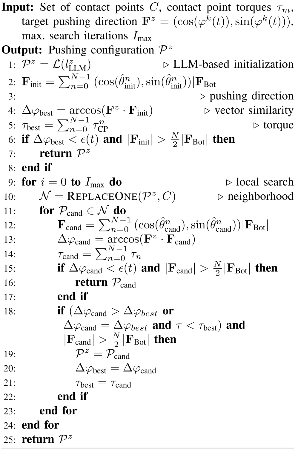
The zero-shot prompt gives the task, desired direction and all candidate world-frame positions and pushing angles. A structured response contains reasoning plus distinct contact indices. The initial configuration is accepted if its net force aligns within the tolerance of Equation 8 and its magnitude exceeds half the team’s nominal total pushing force. The threshold is an assumption, not an inferred object-weight requirement.
If needed, a local step randomly chooses one currently selected contact and tries replacing it with each unused candidate. The prose describes keeping a better aligned feasible configuration, using torque to discourage rotation. Search stops when the directional tolerance is met or the iteration budget expires; experiments use Iₘₐₓ=5. The stated bound is Iₘₐₓ(M−N)+1 evaluated configurations, excluding the LLM’s inference cost.
The preserved Algorithm 1 has important specification inconsistencies: its improvement condition uses Δφcand > Δφbest, opposite to the prose’s smaller-angle objective; its arccos expressions omit normalization of the summed force; and its loop is written from zero through Iₘₐₓ despite the stated iteration bound. Torque notation also varies. These are source ambiguities to resolve against an implementation, not equations silently corrected here.
If the budget expires, the pseudocode returns the current configuration without a final feasibility certificate. Structured output also does not guarantee the correct number of contacts: this causes observed failures. The supplied manuscript describes the prompt but does not include its complete wording or an accessible prompt link.
Equations 7–8
| (7) |
| (8) |
IV-D Online Adaptation
Contacts are reselected when the next key waypoint is reached, deviation from the original path exceeds dᵣₑₚₗ, or progress stalls for tᵣₑₚₗ. This closed loop compensates for some slipping and model error without estimating contact dynamics.
The angle tolerance arctan2(dᵣₑₚₗ, distance to the next waypoint) narrows for distant targets. Its interpretation assumes the ideal pushing direction persists along the segment; real disturbances can still trigger replanning. Numerical replanning thresholds and several controller/spacing parameters are not specified in this manuscript.
IV-E Contact Point Switching
Following Tang and colleagues [5], robot and contact positions are projected onto a circle about the object. A dividing angle balances robots and target contacts on the two semicircles; clockwise ordering then gives the assignment. Under free movement, the assignment avoids inter-robot crossings and bounds travel by half the object perimeter.
Robots realign, plan A* paths to assigned contacts and track them using adaptive pure pursuit [18]. Switching is concurrent only when every planned path is shorter than half the perimeter and at most one robot is near a concave corner; otherwise robots switch sequentially. The free-space assignment property does not guarantee collision avoidance in clutter or near concave bottlenecks, as the full-system results demonstrate.
IV-F Pushing
Proportional controllers prioritize keeping the robot against the boundary rather than exactly preserving its assigned contact location. Equation 9 scales forward motion with distance to the object; Equation 10 combines alignment with the desired pushing orientation and heading toward the assigned contact.
The robots alternate short turning and forward-motion steps to avoid unintended forces during curved motion. This makes the execution approximate even when the selected ideal force vectors satisfy the selector’s conditions; the equations are retained with the source’s notation.
Equations 9–10
| (9) |
| (10) |
V EXPERIMENTS
Evaluation separates the quality and cost of selecting contacts from the difficulty of physically switching to those contacts in the simulator. This distinction is essential when interpreting the high success rates and the scalability plot.
V-A Setup
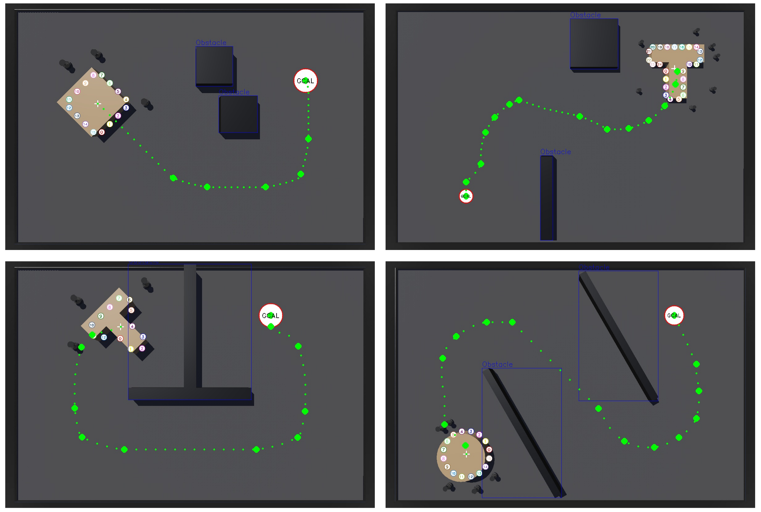
Webots [19] simulates TurtleBot 4 teams of 3, 5, 7, 10, 12 or 15 robots. Five base scenes use a 10×15 m arena. Shapes are a 2×2 m cuboid, a radius-1 m cylinder, and a T with 2.2×0.75 m horizontal and 0.75×1.5 m vertical bars. Base height is 0.5 m and the reported density is 1 kg/m³. For N>4, arena, obstacle and object dimensions are scaled by N/4.
Maximum speeds are 0.2 m/s pushing, 0.1 m/s switching and 1 rad/s turning. Robot–object and ground friction are 0.5 and 1.0. Success requires the object center within 0.5 m of the goal. Computation uses a Ryzen 9 7900 CPU and RTX 4080 GPU. The changing scene/object scale means increasing N also changes path length and transport geometry, rather than isolating robot count alone.
V-B Baselines
Both baselines use the same surrounding pipeline. Their difference is how a pushing configuration is selected.
Naive LLM-based Baseline (N-LLM)
N-LLM executes the raw structured LLM contact list without local refinement. Comparing it with ConPoSe tests the value of the bounded search following the proposal. There is no random-start local-search ablation, so the experiments do not isolate how necessary the LLM initialization is relative to a cheaper heuristic.

Analytical Baseline (A-BL)
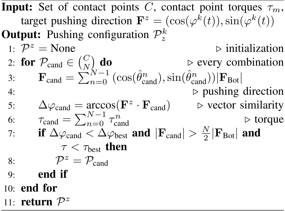
A-BL enumerates all binomial(M,N) distinct contact subsets and evaluates the summed force direction, force magnitude and torque. This is exhaustive search over the discretized candidates, not a complete physical dynamics optimizer. Its cost grows rapidly in the tested regime where N and M increase together; O(2ᴹ) is a broad bound, while the exact enumeration count is binomial(M,N).
Algorithm 2 is retained exactly. It omits initialization and updates of the “best” comparison variables, uses an unnormalized force dot product inside arccos, and combines angular and torque conditions in a way that does not fully specify the prose’s intended ranking. Reproduction requires clarifying those details rather than treating the pseudocode as executable reference code.
V-C Evaluation Metrics
Success rate is the fraction reaching the goal. Z counts selected pushing configurations, Tsel measures selection time per configuration, Texe is total run duration, and Tsw measures switching time per change. Selection time includes LLM service latency; total duration depends on path length, failures and the switching regime. A low Z or short failed run is not necessarily efficient successful transport.
V-D LLM Comparison
Five three-robot cuboid scenes screen language models using N-LLM. GPT-4.1 succeeds in four of five scenes with mean selection time 5.12±0.53 s; GPT-5 succeeds in five with 127.87±18.86 s; o4-mini succeeds in four with 33.85±1.76 s. Gemma 3 and LLaVa succeed in none. A-BL succeeds in five with 0.01 s selection time.
The authors choose GPT-4.1 for subsequent experiments because it balances latency and success in this small screen. This is a task-specific, service-dependent comparison, not a general ranking of model reasoning. There is only one run per scene in the described screen, with no reported repeatability study.
V-E Pushing Configuration Selection Evaluation
The following selection experiments automatically reposition robots at their chosen contacts. They deliberately remove contact-switching failures, so their success rates do not describe the complete executable pipeline.
V-E 1 Scalability
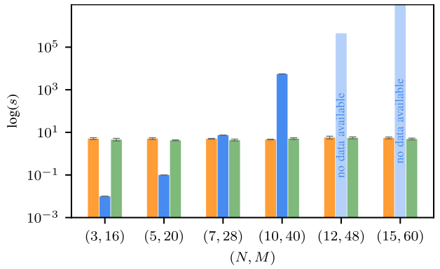
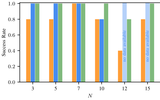
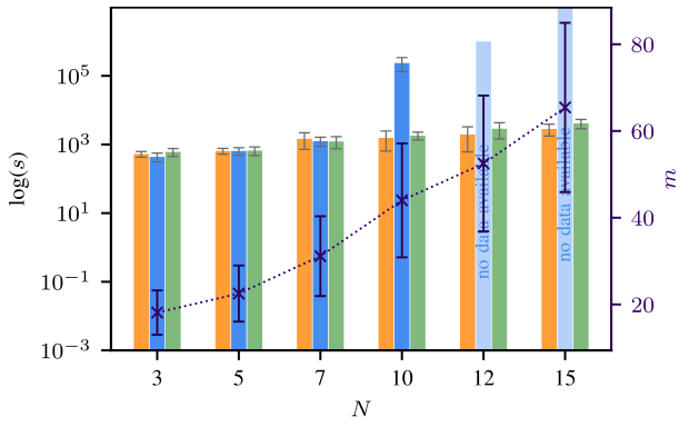
Each selector is tested once in each of five scaled cuboid scenes for each team size. Thus a single failure changes the displayed success rate by twenty percentage points. The candidate counts shown in Figure 4 are 16, 20, 28, 40, 48 and 60 for the six increasing team sizes.
Selection Time
Observed ConPoSe and N-LLM selection latencies stay approximately flat over the tested sizes, with server variability sometimes making the hybrid faster despite its added search. This is an empirical range result, not constant asymptotic complexity: the bounded neighborhood still grows with M−N.
Exhaustive A-BL needs over an hour per selection at ten robots and is described as requiring days at twelve. Completed success and execution measurements are unavailable above ten robots; Figure 4 marks the missing baseline data rather than reporting successful larger-team runs.
Success Rate
ConPoSe succeeds in all five scenes at each size except twelve robots, where one wrong-cardinality LLM proposal causes failure. Its reported range is therefore 80–100%. A-BL has one failure at ten robots after ten consecutive configurations make no meaningful progress; larger baseline runs are not completed. N-LLM success varies substantially, with incorrect contact counts a main failure mode.
Execution Time
Path length grows with scene scale, and mean key-waypoint counts rise from 9.80 to 19.00 between three and fifteen robots. ConPoSe and N-LLM execution times grow moderately, while A-BL becomes dominated by enumeration. Around seven robots the hybrid becomes competitive in selection latency; at ten and above the analytical cost is the main obstacle.
These timing conclusions belong to the automatic-repositioning setting. The paper expects the selector’s advantage to persist with real switching, but does not run the full pipeline above seven robots.
V-E 2 Different Object Shapes
Across five scenes and teams of three, five and seven, ConPoSe and A-BL both score 100% for cuboids and cylinders and 93% for T-shapes. The prose says ConPoSe is slightly worse on the T-shape, but Table II displays the same rounded rate for both. N-LLM scores 87%, 100% and 67%, respectively.
A-BL has the fewest configurations and fastest cuboid/cylinder times. The T-shape row does not follow the prose’s blanket timing ranking: N-LLM is 10.0 min, A-BL 11.7 and ConPoSe 13.5. Lower success can make such duration comparisons misleading. There is no numerical larger-team shape comparison; the claimed crossover there is extrapolated from cuboid scalability.
Cylinders are easiest because inward-normal forces point toward the center and rotation does not change the footprint. All selectors still use more configurations than key waypoints, consistent with extra adaptation to slipping and friction rather than exact ideal-force tracking.
V-F Full System Evaluation
With actual simulated switching, all methods achieve 80% cuboid success. Cylinder success is 80% for ConPoSe and 87% for both baselines. For the T-shape, ConPoSe drops to 7% (one of fifteen runs), N-LLM to 20% (three), and A-BL to 47% (seven). These results sharply qualify the abstract’s near-perfect selection success.
Concave corners and limited room obstruct repositioning. The paper attributes A-BL’s advantage partly to fewer switches and fewer difficult corner configurations, but does not isolate these mechanisms experimentally. The assignment’s free-movement guarantee is insufficient for these constrained situations.
Cuboid total times are 37.8 min for ConPoSe, 46.2 for N-LLM and 35.3 for A-BL; cylinder times are 28.4, 30.4 and 27.3. Switching costs 1.2–2.2 min per change. Every Table III metric includes failed runs: ConPoSe’s apparently best T-shape time of 18.8 min and lowest Z of 8.2 accompany its worst success rate, so they cannot be read as superior transport efficiency.
The full pipeline is tested only up to seven robots. Generalization of its selector’s computational advantage to larger executable teams remains an expectation, not a measured end-to-end result.
VI CONCLUSION
The useful contribution is a practical proposal-plus-search strategy that reduces contact-selection cost in the tested combinatorial regime. The full system’s main bottleneck is robust contact switching with nonholonomic robots, especially around concave objects. Source pseudocode inconsistencies, missing parameter/prompt details, small per-condition trial counts and the absent random-initialization ablation also limit reproducibility and causal attribution.
The conclusion mentions preliminary physical experiments but reports no hardware protocol, trial counts or quantitative results. Grounding DINO and SAM 2 are suggested ways to infer geometry [20][21]; they are not evaluated components of this system. Perception uncertainty, arbitrary mass distributions, dynamic obstacles and reliable large-team switching remain outside the demonstrated scope.
ACKNOWLEDGMENTS
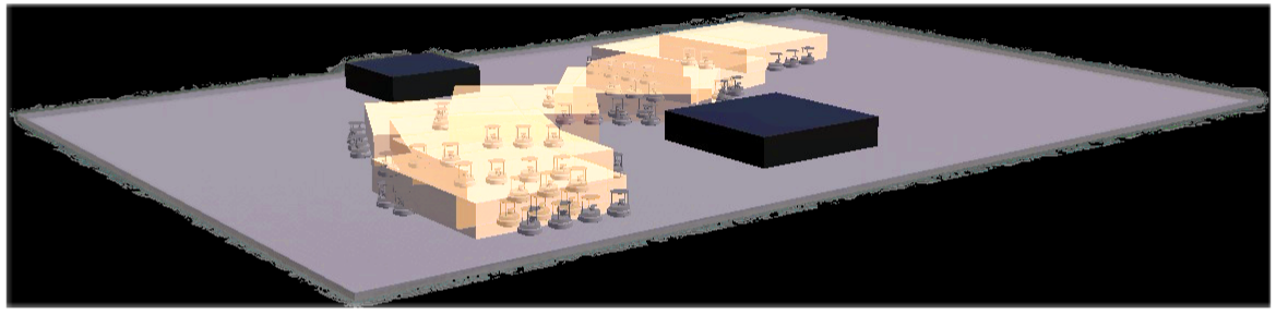
Lucas Kaiser is acknowledged for help creating Figure 1.