The preserved experimental figures compare density-related scores on synthetic distributions, controlled visual data and pretrained image/multimodal encoders. They support the proposed score as a useful diagnostic in those settings. They do not remove the assumptions needed to interpret an encoder-derived score as a normalized input probability.
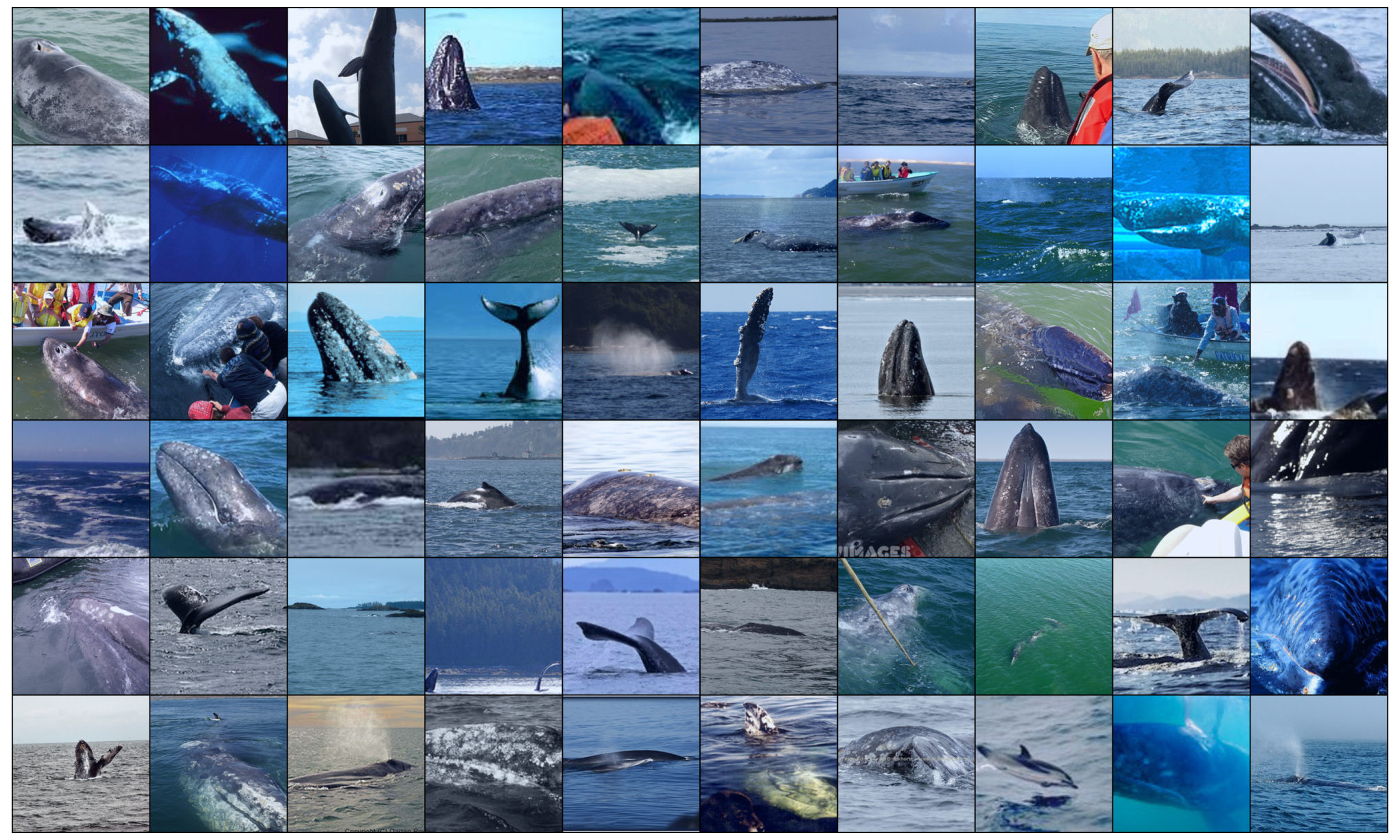
Figure 1: Depiction of the 5 least (left) and 5 most (right) likely samples of class 21 from Imagenet as per JEPA-SCORE–JEPAs’ implicit density estimator learned during pretraining. Two striking observations: (i) across all JEPAs (rows) the type of samples with low and high probabilities are alike, and (ii) the same samples (amongst 1,000) are found at those extrema. Random samples from that class are provided in fig.4
At a glance
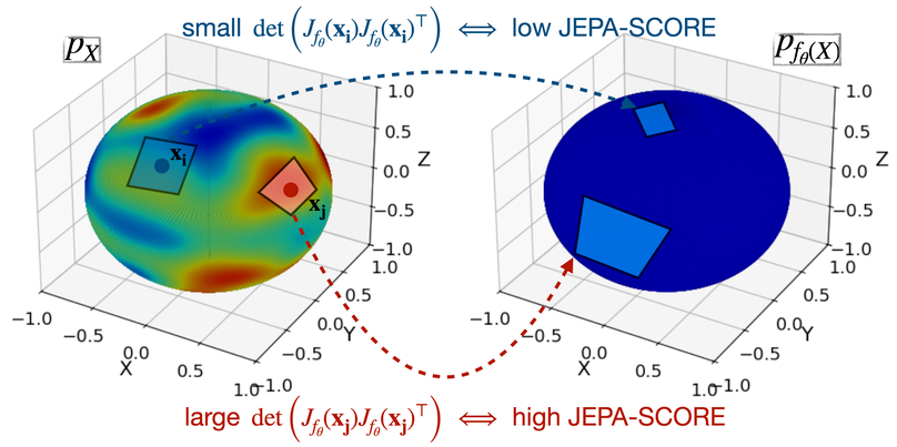
Intuition. Imagine stretching a crowded region of data into a more evenly spread feature space. The amount of local stretching contains information about how crowded the original region was. JEPA-SCORE uses this idea: examine the encoder’s local derivative, or Jacobian, when its output distribution is encouraged to be Gaussian.
The result is a density-related scalar that can help with ranking or curation. Recovering a full input density is more delicate when several distinct inputs map to the same embedding. The paper explicitly permits ambiguity within such sets, and its strongest recovery claim assumes an optimally satisfied JEPA objective and a specified view-generation model.
1 Introduction
The paper connects representation learning with density estimation. A Gaussian distribution maximizes differential entropy under a covariance constraint, motivating the study of encoders with Gaussian-like outputs. The new question is what the local transformation into that distribution reveals about the original data. A non-generative training objective may still carry density information, but that is different from providing an unrestricted, calibrated probability for every input.
The argument proceeds from high-dimensional Gaussian geometry to a change-of-variables relation and then a JEPA-specific score. Each step adds assumptions; the final estimator should be read together with those assumptions.
2.1 Preliminaries: Gaussian Embeddings Are Uniform on the Hypersphere
A high-dimensional isotropic Gaussian has uniformly distributed directions and a radius concentrated near a predictable value after scaling. The uniform direction is an exact symmetry; concentration near a sphere is a high-dimensional approximation. A finite-dimensional Gaussian is not literally the same distribution as a surface-only uniform law.
Lemma 1.
As grows, quickly concentrates around the hypersphere of radius , converging to a Uniform density over the hypersphere surface. (Proof in sectionA.1.)
2.2 Producing Gaussian Embeddings Equates Learning an Energy Function
For an invertible map, input and output densities are related by local volume change, measured by the Jacobian. For a many-to-one encoder, the relation integrates over all inputs sharing an embedding. The output distribution therefore constrains density averaged along these level sets, while allowing ambiguity within each set. This is why Gaussian output alone cannot uniquely determine arbitrary pointwise input probabilities.
Equation 1
(1)
Lemma 2.
In order for to be distributed as for large , must learn the data density up to mean-preserving rescaling within each level-set . (Proof in sectionA.2.)
512
1024
2048
4096
dim
64
0.64
0.69
0.84
0.90
128
0.75
0.85
0.90
0.94
256
0.82
0.83
0.69
0.76
512
0.72
0.75
0.84
0.88
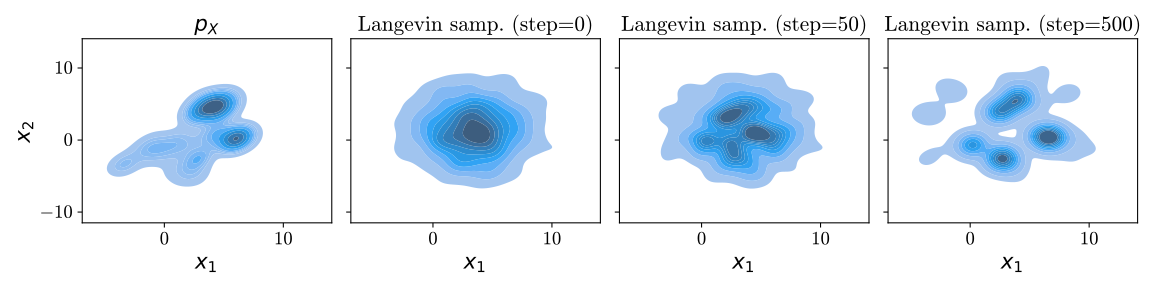
Figure 2: Top left: Visual illustration of JEPA-SCORE–the DN must learn for its Jacobian matrix to expand or contract the density in order to produce a Uniform density on the hypersphere surface in its embedding space (lemmas1 and 2). Top right: Pearson correlation between JEPA-SCORE and the true on a GMM data model for various input dimensions (rows) and number of samples (columns). In all cases, producing Gaussian embeddings make the backbone internalize the data density which can be easily extracted using our proposed JEPA-SCORE. Bottom: as JEPA-SCORE is an approximation of the true score function, it is possible to perform Langevin sample to recover the true data distribution as shown here in two dimensions.
The JEPA-specific derivation models each sample as a stochastic transformation of an underlying generator and links view invariance to encoder level sets. At the stated optimum, the resulting expression estimates the generator density. JEPA-SCORE uses Jacobian singular values and a Monte Carlo estimate, often reported on a log scale. In practical networks, finite training error, approximate Gaussianity, transformation assumptions and numerical estimation qualify the density interpretation. Here “score” names the proposed scalar estimator; it should not be confused with automatically possessing a perfect generative model.
Equations 2–3
(2)
(3)
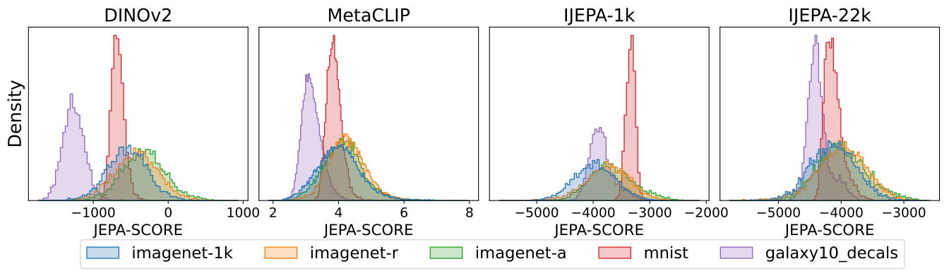
Figure 3: Depiction of JEPA-SCORE for samples from different datasets (imagenet-1k/a/r, MNIST and Galaxy). We clearly observe that as the pretraining dataset size increases (all models against IJEPA-1k) as MNIST and Galaxy images are seen as lower probability samples, i.e., those images are less and less represented within the overall pretraining dataset. While our score does not rely on singular vectors, we provide some examples in fig.7. This can be used to assess if a model is ready or not to handle particular data domains at test time for zero-shot tasks.
Theorem 1.
At optimality, JEPA embeddings estimate the data density as per
Equation 4
(4)
Equation 5
(5)
Appendix A Proofs
A.1 Proof of lemma 1
The proof separates Gaussian radius and direction in spherical coordinates. The normalized squared radius has variance decreasing with dimension, explaining shell concentration. Directional uniformity follows from rotational symmetry.
Equations
(Cartesian coordinates)
(Cartesian coordinates)
A.2 Proof of lemma 2
The proof uses the coarea/change-of-variables relation. With a bijection, local volume change directly relates densities. With a non-injective map, probability can redistribute within a level set while leaving its integrated output contribution unchanged. This ambiguity is part of the result.
A.3 Proof of theorem 1
The theorem connects the assumed transformation-induced view relation with encoder level sets, then substitutes it into the density relation. Its optimum and transformation-model assumptions matter when moving from the formal expression to a trained checkpoint.
Equations
Appendix B Implementation Details
The preserved implementation blocks give the numerical construction of the proposed estimator. Jacobian computation and singular-value handling are part of its cost and numerical behavior; the absence of a pixel decoder does not make this calculation free.
Listing 1: JEPA-SCORE implementation in PyTorch. Our empirical ablations demonstrate that JEPA-SCORE is not sensitive to the choice of eps (we pick )
Appendix C Additional Figures
The additional original plots extend the controlled density and representation comparisons. Use them as empirical checks of the stated settings, rather than as proof that any arbitrary self-supervised model supplies calibrated probabilities.
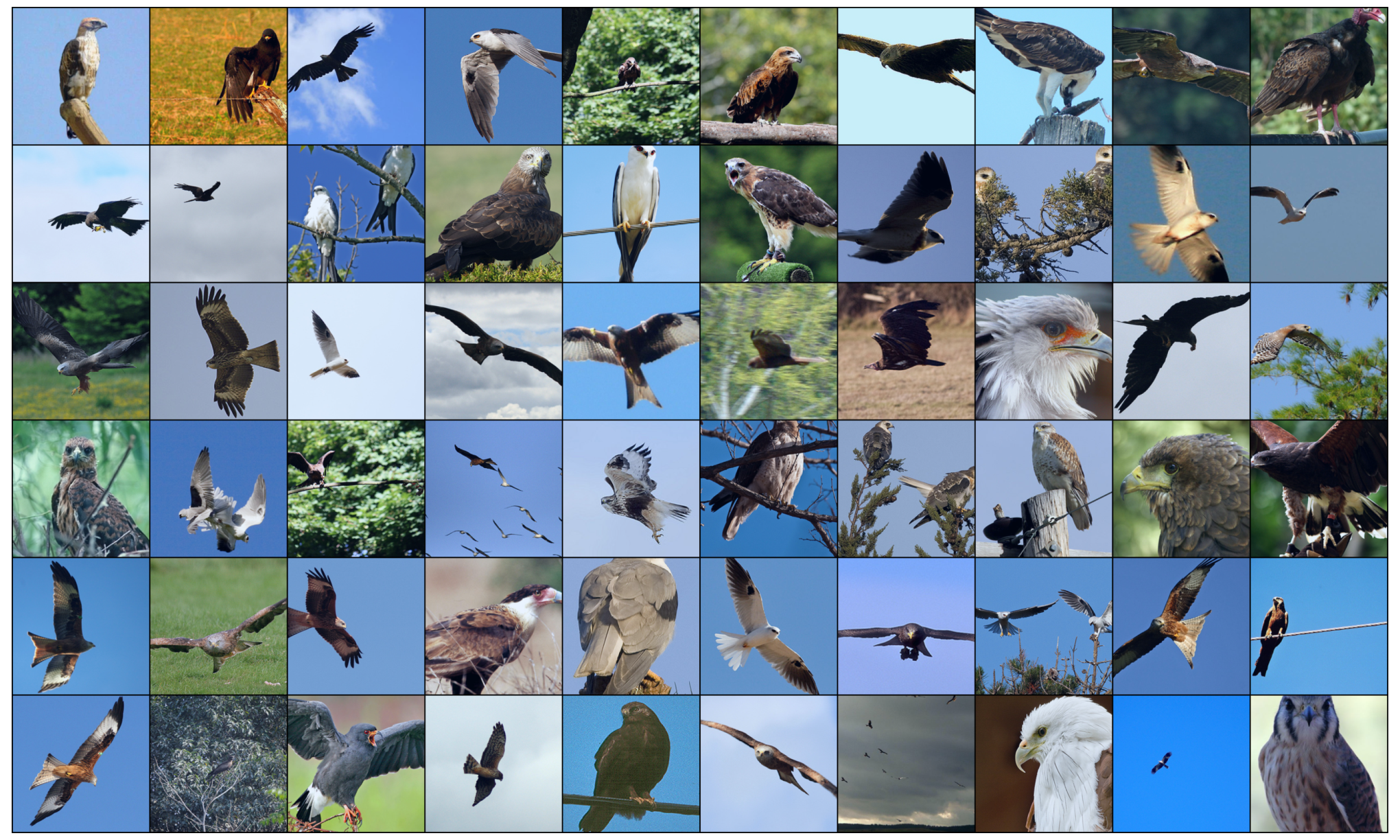
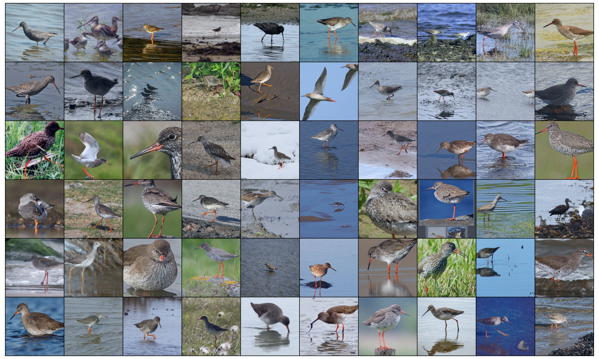
Figure 4: Random samples from Imagenet-1k training dataset for class 21.
Figure 5: Top: least and most likely samples based on the proposed JEPA-SCORE for a fe different pretrained backbones on class 141. Bottom:Random samples from Imagenet-1k training dataset for class 141.
Figure 6: Top: least and most likely samples based on the proposed JEPA-SCORE for a fe different pretrained backbones on class 141. Bottom:Random samples from Imagenet-1k training dataset for class 147.
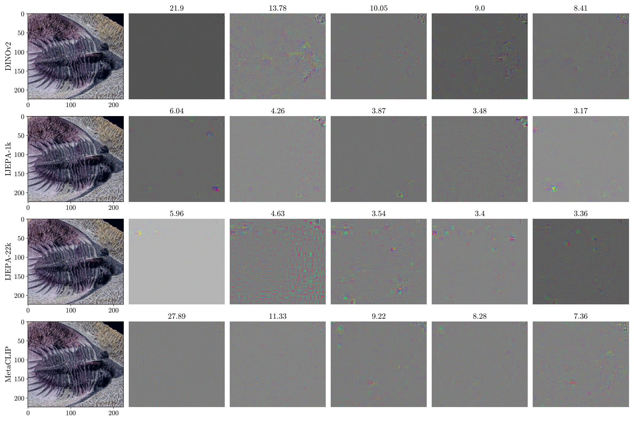
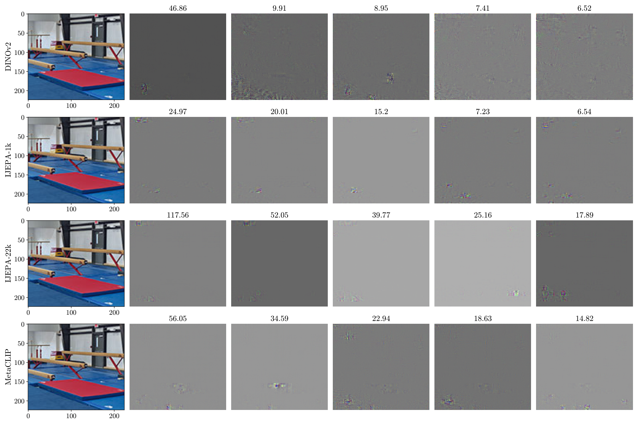
Figure 7: Depiction of the top singular vectors of the Jacobian matrix (columns) for a given input image (left column). The corresponding singular value is provided in the title of each subplot.
17 references
(1)
Mahmoud Assran, Quentin Duval, Ishan Misra, Piotr Bojanowski, Pascal Vincent, Michael Rabbat, Yann LeCun, and Nicolas Ballas.
Self-supervised learning from images with a joint-embedding predictive architecture.
In Proceedings of the IEEE/CVF Conference on Computer Vision and Pattern Recognition, pages 15619–15629, 2023.
(3)
Randall Balestriero and Yann LeCun.
Learning by reconstruction produces uninformative features for perception.
arXiv preprint arXiv:2402.11337, 2024.
(5)
Mathilde Caron, Hugo Touvron, Ishan Misra, Hervé Jégou, Julien Mairal, Piotr Bojanowski, and Armand Joulin.
Emerging properties in self-supervised vision transformers.
In Proceedings of the IEEE/CVF international conference on computer vision, pages 9650–9660, 2021.
(6)
Ting Chen, Simon Kornblith, Mohammad Norouzi, and Geoffrey Hinton.
A simple framework for contrastive learning of visual representations.
In International conference on machine learning, pages 1597–1607. PmLR, 2020.
(7)
Milan Cvitkovic and Günther Koliander.
Minimal achievable sufficient statistic learning.
In International Conference on Machine Learning, pages 1465–1474. PMLR, 2019.
(8)
Aleksandr Ermolov, Aliaksandr Siarohin, Enver Sangineto, and Nicu Sebe.
Whitening for self-supervised representation learning.
In International conference on machine learning, pages 3015–3024. PMLR, 2021.
(9)
Kaiming He, Haoqi Fan, Yuxin Wu, Saining Xie, and Ross Girshick.
Momentum contrast for unsupervised visual representation learning.
In Proceedings of the IEEE/CVF conference on computer vision and pattern recognition, pages 9729–9738, 2020.
(10)
R Devon Hjelm, Alex Fedorov, Samuel Lavoie-Marchildon, Karan Grewal, Phil Bachman, Adam Trischler, and Yoshua Bengio.
Learning deep representations by mutual information estimation and maximization.
arXiv preprint arXiv:1808.06670, 2018.
(13)
Etai Littwin, Omid Saremi, Madhu Advani, Vimal Thilak, Preetum Nakkiran, Chen Huang, and Joshua Susskind.
How jepa avoids noisy features: The implicit bias of deep linear self distillation networks.
Advances in Neural Information Processing Systems, 37:91300–91336, 2024.
(14)
Alec Radford, Jong Wook Kim, Chris Hallacy, Aditya Ramesh, Gabriel Goh, Sandhini Agarwal, Girish Sastry, Amanda Askell, Pamela Mishkin, Jack Clark, et al.
Learning transferable visual models from natural language supervision.
In International conference on machine learning, pages 8748–8763. PmLR, 2021.
(15)
Manu Srinath Halvagal, Axel Laborieux, and Friedemann Zenke.
Implicit variance regularization in non-contrastive ssl.
Advances in Neural Information Processing Systems, 36:63409–63436, 2023.
(16)
Pascal Vincent, Hugo Larochelle, Yoshua Bengio, and Pierre-Antoine Manzagol.
Extracting and composing robust features with denoising autoencoders.
In Proceedings of the 25th international conference on Machine learning, pages 1096–1103, 2008.
(17)
Tongzhou Wang and Phillip Isola.
Understanding contrastive representation learning through alignment and uniformity on the hypersphere.
In International conference on machine learning, pages 9929–9939. PMLR, 2020.