Overview
This edition follows the complete 18-page v2 manuscript dated July 27, 2026, with all eight listed authors. It preserves seven numbered figures, seven tables, seven displayed equations and 47 references. PDF-derived composites restore the teaser and retain native imagery and vector labels. The manuscript mentions a separate Supplementary Figure C1 that is absent from this PDF and linked project page; no claim is made to reproduce that unavailable supplement.
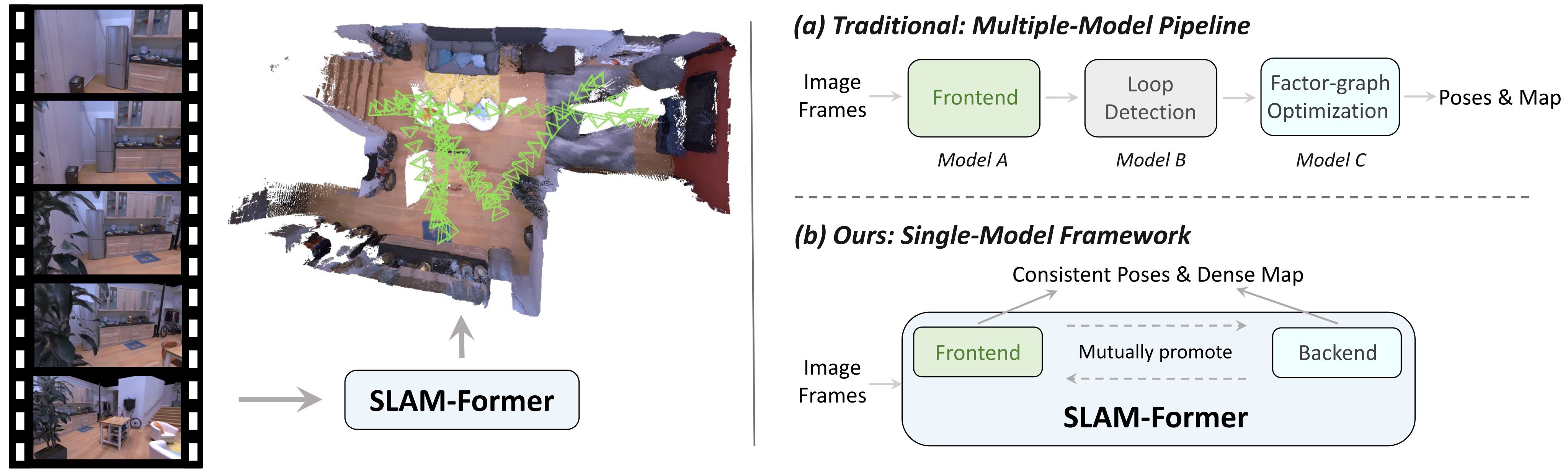
At a glance
SLAM-Former shares one transformer between incremental monocular tracking/mapping and periodic global refinement. The frontend creates map tokens and an attention cache; the backend revisits those tokens and replaces the cache used for later frames. Training covers causal, mixed and full attention so the two operations can cooperate. It gives the best average uncalibrated trajectory error in the reported indoor benchmarks and strong dense reconstruction, while remaining dependent on growing memory, expensive global passes and learned geometric priors.
1 Introduction
Dense monocular SLAM must estimate both camera motion and scene geometry from an image stream. Pairwise or submap-based learned systems can retain seams between local reconstructions; purely streaming models can accumulate drift because they do not revise earlier predictions. SLAM-Former addresses these limitations by alternating incremental inference and global token refinement.
One shared backbone performs both roles, with separate geometry and pose heads. Full cross-frame attention replaces an explicit loop-detection and pose-graph module. Calling this equivalent to loop closure describes its intended function, not a proof of geometric consistency, place recognition accuracy or recovery after tracking loss. The paper evaluates those effects through trajectory and reconstruction errors.
2 Related Works
The related work contrasts dense SLAM pipelines that combine learned geometry with explicit optimization, feed-forward multi-view reconstruction, and streaming models with persistent memory.
2.1 Dense RGB SLAM
CodeSLAM and DeepFactors optimize compact depth representations; DROID-SLAM combines learned correspondence with bundle adjustment [3][6][32]. Neural radiance-field and Gaussian representations focus on rendering as well as mapping. The source criticizes their geometric reliability broadly, but their behavior depends on the representation and evaluation; these methods should not be treated as incapable of representing geometry.
MASt3R-SLAM uses pairwise reconstruction priors [25], while VGGT-SLAM connects submaps through a projective transformation model [22]. SLAM-Former instead lets all retained map tokens interact in a shared neural backend. This is a different mechanism for global correction, not an assertion that previous SLAM systems lack global optimization.
2.2 Feed-forward 3D Reconstruction
DUSt3R estimates pairwise geometry [36]. Fast3R, VGGT and Pi3 extend direct inference to multiple views [39][34][37]. Streaming approaches such as Spann3R, CUT3R, LONG3R and StreamVGGT trade global revisiting for efficient online state updates [33][35][5][47]. SLAM-Former combines streaming frontend work with periodic revision of the entire retained map.
3 SLAM-Former
The method uses a shared transformer, persistent map tokens, attention-cache exchange, three training configurations and a pruning scheme for reducing attention cost. Its online schedule is separate from its batched training schedule.
3.1 Transformer Architecture
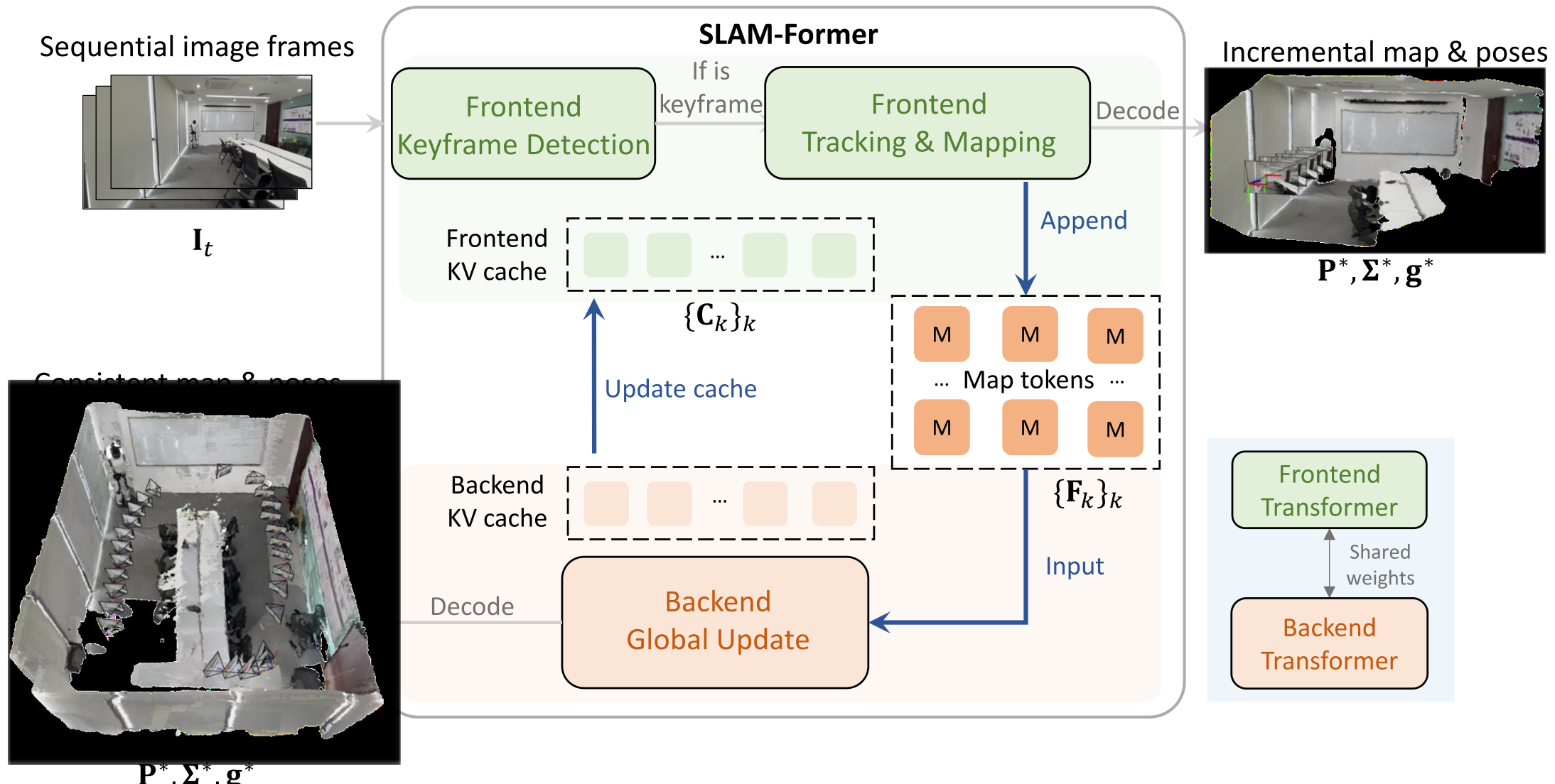
A pretrained image encoder supplies patch tokens augmented by register tokens. The backbone alternates within-frame and cross-frame attention, and task heads decode local pointmaps, confidence and camera poses. “One transformer” refers to the shared frontend/backend backbone; the image encoder and output heads remain distinct components. Figure 2 preserves the complete data flow.
3.2 Frontend
Given a new image and cached keys/values from previous keyframes, the frontend produces map tokens, as in Equation 1. These tokens represent geometry implicitly and can be decoded into a pointmap, confidence map and camera pose. A confirmed keyframe adds both its map tokens and its attention cache to persistent state.
Equation 1
| (1) |
Keyframe Detection.
In the implemented keyframe detector, the current image and latest keyframe are processed together without the accumulated cache. Their relative pose determines whether motion exceeds the selection threshold. This lightweight pairwise check precedes the more expensive cached tracking/mapping pass; the implementation specifies a translation threshold of 0.1, rather than a fully described rotation/translation criterion.
Frontend Tracking and Mapping.
For a selected keyframe, the frontend recomputes its tokens using all retained previous cache entries, then appends the result and keyframe index through Equation 2. Dependence only on past frames makes this stage causal. Its estimates can still drift, motivating the backend’s later revision.
Equation 2
| (2) |
3.3 Backend
The backend feeds the accumulated map tokens through the same backbone using full attention. Equation 3 produces refined map tokens in one forward pass, allowing distant frames to influence one another. This learned correction can reduce seams and drift, but full attention does not itself impose a hard geometric consistency constraint.
Equation 3
| (3) |
Cache Sharing.
The backend’s newly computed keys and values replace the frontend’s stored cache. Later frames are therefore processed against the revised global representation instead of the older causal estimates. This feedback makes the backend useful beyond polishing the final map.
3.4 Training Strategy
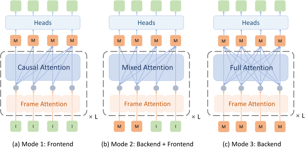
Each training iteration executes three modes with shared weights: causal frontend processing, a mixed backend/frontend configuration, and full-attention backend refinement. Their masks reproduce the corresponding cache dependencies at inference. Figure 3 retains both the architecture and the small visual symbols used to distinguish image tokens, map tokens and intermediate outputs.
Training Frontend.
Mode 1 uses causal cross-frame attention, so each frame depends only on earlier frames. Batched training learns the same attention dependency structure as incremental inference with an accumulated key–value cache.
Training Frontend with Backend Cooperation.
Mode 2 combines previously generated map tokens and new image tokens. Map tokens interact with full attention; new frames attend causally while accessing the backend-derived context. This trains the cache-sharing interface rather than assuming a purely causal model can consume a globally refined cache without adjustment.
Training Backend.
Mode 3 refines map tokens produced under different earlier runs or cache states. Full attention lets the model revise their collective geometry. The paper does not provide a separate ablation for every training mode, so their individual contributions are not isolated.
Joint Training.
Output pointmaps are local to each frame, avoiding a fixed world-reference requirement. Depth supervision combines confidence-weighted residuals and spatial-gradient residuals with a log-confidence regularizer; a fitted scale aligns predictions to ground truth. Pointmap supervision transforms local predictions relative to the first frame, while the camera objective applies a Huber loss to relative poses with scaled translations.
Equations 4–6 preserve the exact source losses. The per-mode objective is depth loss plus pointmap loss plus λ times camera loss; all three mode losses are then combined as L₁ + L₂ + βL₃. Training uses λ=100 and β=10. Scale alignment is part of the loss, so these results should not be read as a proof that arbitrary monocular scenes have physically determined metric scale.
Equations 4–6
| (4) |
| (5) |
| (6) |
3.5 Execution Pipeline
At inference, keyframe selection and incremental tracking run between periodic global passes. Both operations use the same trained backbone with different inputs and attention dependencies.
Frontend.
The first two selected keyframes initialize map tokens and caches jointly. Each later selected keyframe uses the cached history; non-keyframes are not appended to the global map. Keyframe selection itself uses a two-image full-attention pose estimate.
Backend.
After every ten keyframes, the backend refines all accumulated map tokens and refreshes their cache entries. This is periodic global work, not a constant-cost update, and its latency grows with the retained history.
3.6 KV Pruning for Runtime Efficiency
Following DivPrune [1], Equation 7 chooses a diverse subset of non-register patch tokens by maximizing minimum pairwise cosine distance. Greedy selection approximates that subset with a per-frame quadratic pairwise-distance precomputation. Only keys and values are pruned; all queries remain, preserving dense output locations.
A fixed retention fraction γ reduces the dominant frontend and backend attention terms to O(γn) and O(γn²). A constant factor does not change their asymptotic orders. Shrinking the retained fraction as history grows can instead give sublinear frontend attention and lower-order backend attention; logarithmic or square-root cache schedules produce the stated O(n log n) or O(n¹·⁵) backend terms. These bounds describe attention work and omit other compute, selection overhead and persistent map storage.
Equation 7
| (7) |
4 Experiments
Experiments report trajectory accuracy on TUM RGB-D, 7-Scenes and Replica, dense reconstruction on the latter two, a frontend/backend ablation, and cache-pruning speed/accuracy curves. All are benchmark evaluations; there is no reported autonomous-navigation deployment.
4.1 Experimental Setup
Training uses multiple indoor and multi-view datasets. Evaluation distinguishes methods supplied with camera calibration from those operating without it, and mixes source-reported results with runs performed by the authors.
Implementation Details.
The 36-layer backbone starts from Pi3 weights [37]. Training freezes the image encoder and camera head, uses batches of 32 containing twelve frames each, and runs ten epochs with AdamW at 10⁻⁵ learning rate and cosine decay. It takes eleven hours on 32 A100 GPUs; inference measurements use one RTX 4090.
Training data comprises ARKitScenes, ScanNet, ScanNet++, HyperSim, BlendedMVS, MegaDepth and MVS-Synth. Test sequences are longer than the twelve-frame training clips. The 0.1 translation threshold and ten-keyframe backend interval define the reported schedule; pruning is disabled unless specified.
Baselines.
Baselines include calibrated and uncalibrated SLAM methods plus streaming reconstruction models. CUT3R and StreamVGGT use the authors’ selected keyframes, while starred table entries come from prior publications and plus-marked entries are rerun. This mixed provenance limits strict implementation-level fairness.
Some original table reference labels are mismatched: Table 1’s ORB-SLAM3 row cites the older ORB-SLAM reference, Table 2’s VGGT-SLAM row cites VGGT, and Table 3’s uncalibrated DROID-SLAM row cites DUSt3R. The rows and numbers are preserved; the intended methods are identified by their names, with correct primary references [4][22][32].
| Method | Sequence | Avg | |||||||||
|---|---|---|---|---|---|---|---|---|---|---|---|
| 360 | desk | desk2 | floor | plant | room | rpy | teddy | xyz | |||
| Calib. | ORB-SLAM3 [24] | 0.017 | 0.210 | 0.034 | 0.009 | N/A | |||||
| DeepV2D [31] | 0.243 | 0.166 | 0.379 | 1.653 | 0.203 | 0.246 | 0.105 | 0.316 | 0.064 | 0.375 | |
| DeepFactors [6] | 0.159 | 0.170 | 0.253 | 0.169 | 0.305 | 0.364 | 0.043 | 0.601 | 0.035 | 0.233 | |
| DPV-SLAM [20] | 0.112 | 0.018 | 0.029 | 0.057 | 0.021 | 0.330 | 0.030 | 0.084 | 0.010 | 0.076 | |
| DPV-SLAM++ [20] | 0.132 | 0.018 | 0.029 | 0.050 | 0.022 | 0.096 | 0.032 | 0.098 | 0.010 | 0.054 | |
| GO-SLAM [45] | 0.089 | 0.016 | 0.028 | 0.025 | 0.026 | 0.052 | 0.019 | 0.048 | 0.010 | 0.035 | |
| DROID-SLAM [32] | 0.111 | 0.018 | 0.042 | 0.021 | 0.016 | 0.049 | 0.026 | 0.048 | 0.012 | 0.038 | |
| MASt3R-SLAM [25] | 0.049 | 0.016 | 0.024 | 0.025 | 0.020 | 0.061 | 0.027 | 0.041 | 0.009 | 0.030 | |
| Uncalib. | CUT3R+ [35] | 0.102 | 0.054 | 0.118 | 0.211 | 0.083 | 0.264 | 0.044 | 0.120 | 0.020 | 0.113 |
| StreamVGGT+ [47] | 0.088 | 0.063 | 0.105 | 0.604 | 0.070 | 0.633 | 0.025 | 0.081 | 0.015 | 0.187 | |
| DROID-SLAM* [32] | 0.202 | 0.032 | 0.091 | 0.064 | 0.045 | 0.918 | 0.056 | 0.045 | 0.012 | 0.158 | |
| MASt3R-SLAM* [25] | 0.070 | 0.035 | 0.055 | 0.056 | 0.035 | 0.118 | 0.041 | 0.114 | 0.020 | 0.060 | |
| VGGT-SLAM [22] | 0.071 | 0.025 | 0.040 | 0.141 | 0.023 | 0.102 | 0.030 | 0.034 | 0.014 | 0.053 | |
| EC3R-SLAM [12] | 0.101 | 0.038 | 0.050 | 0.055 | 0.097 | 0.101 | 0.045 | 0.125 | 0.018 | 0.070 | |
| ViSTA-SLAM [44] | 0.104 | 0.030 | 0.030 | 0.070 | 0.052 | 0.067 | 0.023 | 0.080 | 0.015 | 0.052 | |
| Ours | 0.067 | 0.018 | 0.026 | 0.079 | 0.021 | 0.082 | 0.017 | 0.030 | 0.011 | 0.039 | |
4.2 3D Tracking Evaluation
Tracking uses the root mean square absolute trajectory error in meters. Average rankings do not imply that a method wins every sequence, and calibrated and uncalibrated groups should remain distinct.
TUM RGB-D Tracking.
On TUM, SLAM-Former averages 0.039 m, better than all listed uncalibrated alternatives (the closest is ViSTA-SLAM at 0.052 m). It remains behind calibrated MASt3R-SLAM at 0.030 m and GO-SLAM at 0.035 m, and close to calibrated DROID-SLAM at 0.038 m.
The improvement is not uniform: floor error is 0.079 m versus uncalibrated EC3R-SLAM’s 0.055 m, and room error is 0.082 m versus ViSTA-SLAM’s 0.067 m. Thus the narrative’s emphasis on floor/room should not be interpreted as a per-scene win over every competitor.
| Method | Sequence | Avg | |||||||
|---|---|---|---|---|---|---|---|---|---|
| chess | fire | heads | office | pumpkin | kitchen | stairs | |||
| Calib. | NICER-SLAM [46] | 0.033 | 0.069 | 0.042 | 0.108 | 0.200 | 0.039 | 0.108 | 0.086 |
| DROID-SLAM [32] | 0.036 | 0.027 | 0.025 | 0.066 | 0.127 | 0.040 | 0.026 | 0.049 | |
| MASt3R-SLAM [25] | 0.053 | 0.025 | 0.015 | 0.097 | 0.088 | 0.041 | 0.011 | 0.047 | |
| Uncalib. | CUT3R+ [35] | 0.046 | 0.043 | 0.055 | 0.120 | 0.096 | 0.061 | 0.086 | 0.073 |
| StreamVGGT+ [47] | 0.048 | 0.036 | 0.030 | 0.117 | 0.094 | 0.063 | 0.179 | 0.081 | |
| DROID-SLAM* [32] | 0.047 | 0.038 | 0.034 | 0.136 | 0.166 | 0.080 | 0.044 | 0.078 | |
| MASt3R-SLAM* [25] | 0.063 | 0.046 | 0.029 | 0.103 | 0.114 | 0.074 | 0.032 | 0.066 | |
| VGGT-SLAM [34] | 0.036 | 0.028 | 0.018 | 0.103 | 0.133 | 0.058 | 0.093 | 0.067 | |
| EC3R-SLAM [12] | 0.050 | 0.042 | 0.059 | 0.113 | 0.143 | 0.065 | 0.050 | 0.075 | |
| ViSTA-SLAM [44] | 0.073 | 0.035 | 0.028 | 0.055 | 0.129 | 0.035 | 0.029 | 0.055 | |
| Ours | 0.039 | 0.033 | 0.018 | 0.070 | 0.065 | 0.035 | 0.033 | 0.042 | |
7-Scenes Tracking.
On 7-Scenes, the average 0.042 m is the lowest in Table 2, compared with calibrated MASt3R-SLAM’s 0.047 m and DROID-SLAM’s 0.049 m. Pumpkin is a clear gain at 0.065 m. Other sequences favor competitors: office is 0.070 m versus ViSTA-SLAM’s 0.055 m, while kitchen ties it at 0.035 m.
Replica Tracking.
On synthetic Replica, SLAM-Former’s 0.030 m is the best uncalibrated average, about 55% below SLAM3R’s 0.066 m. Calibrated NICER-SLAM scores 0.019 m and DROID-SLAM 0.003 m. The source describes NICER-SLAM as “on par,” but its displayed error is appreciably lower; the learned method is strongest within the uncalibrated comparison. The proposed explanation about clean synthetic imagery is plausible but not separately tested.
| Method | Sequence | Avg | ||||||||
|---|---|---|---|---|---|---|---|---|---|---|
| Rm0 | Rm1 | Rm2 | Of0 | Of1 | Of2 | Of3 | Of4 | |||
| Calib. | NICER-SLAM [46] | 0.013 | 0.016 | 0.011 | 0.021 | 0.032 | 0.021 | 0.014 | 0.020 | 0.019 |
| DROID-SLAM [32] | 0.003 | 0.001 | 0.003 | 0.003 | 0.004 | 0.003 | 0.005 | 0.004 | 0.003 | |
| Uncalib. | SLAM3R [21] | 0.046 | 0.059 | 0.057 | 0.112 | 0.063 | 0.062 | 0.050 | 0.081 | 0.066 |
| CUT3R + [35] | 0.145 | 0.243 | 0.127 | 0.159 | 0.230 | 0.162 | 0.088 | 0.204 | 0.170 | |
| StreamVGGT+ [47] | 0.113 | 0.163 | 0.077 | 0.076 | 0.070 | 0.180 | 0.153 | 0.168 | 0.125 | |
| VGGT-SLAM + [22] | 0.030 | 0.167 | 0.086 | 0.042 | 0.064 | 0.095 | 0.039 | 0.043 | 0.071 | |
| DROID-SLAM [36] | 0.313 | 0.111 | 0.125 | 0.029 | 0.421 | 0.045 | 0.253 | 0.249 | 0.193 | |
| MASt3R-SLAM [25] | 0.023 | 0.035 | 0.103 | 0.038 | 0.033 | 0.047 | 0.035 | 0.045 | 0.045 | |
| EC3R-SLAM [12] | 0.038 | 0.049 | 0.027 | 0.043 | 0.034 | 0.059 | 0.025 | 0.053 | 0.041 | |
| ViSTA-SLAM [44] | 0.069 | 0.093 | 0.136 | 0.074 | 0.193 | 0.118 | 0.049 | 0.130 | 0.108 | |
| Ours | 0.030 | 0.026 | 0.027 | 0.028 | 0.029 | 0.038 | 0.028 | 0.031 | 0.030 | |
4.3 Reconstruction Evaluation
The source follows different reconstruction protocols for 7-Scenes and Replica. Lower point-distance errors are better. Exact results and provenance markings are retained instead of merging the datasets into one scale or comparison.
| Method | 7-Scenes | ||||
|---|---|---|---|---|---|
| ATE | Acc. | Complet. | Chamfer | ||
| Calib. | DROID-SLAM [32] | 0.049 | 0.141 | 0.048 | 0.094 |
| MASt3R-SLAM [25] | 0.047 | 0.089 | 0.085 | 0.087 | |
| Spann3R @20 [33] | N/A | 0.069 | 0.047 | 0.058 | |
| Spann3R @2 [33] | N/A | 0.124 | 0.043 | 0.084 | |
| Uncalib. | CUT3R+ [35] | 0.073 | 0.032 | 0.047 | 0.040 |
| StreamVGGT+ [47] | 0.081 | 0.058 | 0.057 | 0.057 | |
| MASt3R-SLAM* [25] | 0.066 | 0.068 | 0.045 | 0.056 | |
| VGGT-SLAM [22] | 0.067 | 0.052 | 0.058 | 0.055 | |
| EC3R-SLAM [12] | 0.075 | 0.025 | 0.054 | 0.040 | |
| ViSTA-SLAM [44] | 0.056 | 0.051 | 0.055 | 0.045 | |
| Ours | 0.042 | 0.017 | 0.037 | 0.027 | |
| Method | Room 0 | Room 1 | Room 2 | Office 0 | Office 1 | Office 2 | Office 3 | Office 4 | Average |
|---|---|---|---|---|---|---|---|---|---|
| Acc. / Comp. | Acc. / Comp. | Acc. / Comp. | Acc. / Comp. | Acc. / Comp. | Acc. / Comp. | Acc. / Comp. | Acc. / Comp. | Acc. / Comp. | |
| DUSt3R [36] | 3.47 / 2.50 | 2.53 / 1.86 | 2.95 / 1.76 | 4.92 / 3.51 | 3.09 / 2.21 | 4.01 / 3.10 | 3.27 / 2.25 | 3.66 / 2.61 | 3.49 / 2.48 |
| MASt3R [17] | 4.01 / 4.10 | 3.61 / 3.25 | 3.13 / 2.15 | 2.57 / 1.63 | 12.85 / 8.13 | 3.13 / 1.99 | 4.67 / 3.15 | 3.69 / 2.47 | 4.71 / 3.36 |
| NICER-SLAM* [46] | 2.53 / 3.04 | 3.93 / 4.10 | 3.40 / 3.42 | 5.49 / 6.09 | 3.45 / 4.42 | 4.02 / 4.29 | 3.34 / 4.03 | 3.03 / 3.87 | 3.65 / 4.16 |
| DROID-SLAM* [32] | 12.18 / 8.96 | 8.35 / 6.07 | 3.26 / 16.01 | 3.01 / 16.19 | 2.39 / 16.20 | 5.66 / 15.56 | 4.49 / 9.73 | 4.65 / 9.63 | 5.50 / 12.29 |
| DIM-SLAM* [18] | 14.19 / 6.24 | 9.56 / 6.45 | 8.41 / 12.17 | 10.16 / 5.95 | 7.86 / 8.33 | 16.50 / 8.28 | 13.01 / 6.77 | 13.08 / 8.62 | 11.60 / 7.85 |
| GO-SLAM- [45] | - | - | - | - | - | - | - | - | 3.81 / 4.79 |
| Spann3R- [33] | 9.75 / 12.94 | 15.51 / 12.94 | 7.28 / 8.50 | 5.46 / 18.75 | 5.24 / 16.64 | 9.33 / 11.80 | 16.00 / 9.03 | 13.97 / 16.02 | 10.32 / 13.33 |
| SLAM3R- [21] | 3.19 / 2.40 | 3.12 / 2.34 | 2.72 / 2.00 | 4.28 / 2.60 | 3.17 / 2.34 | 3.84 / 2.78 | 3.90 / 3.16 | 4.32 / 3.36 | 3.57 / 2.62 |
| CUT3R+ [35] | 6.09 / 3.09 | 9.89 / 4.55 | 5.77 / 2.66 | 5.23 / 2.46 | 11.60 / 6.94 | 8.00 / 3.16 | 6.12 / 3.09 | 7.46 / 3.05 | 7.52 /3.62 |
| StreamVGGT+ [47] | 9.01 / 4.37 | 12.22 / 4.66 | 5.61 / 2.61 | 6.64 / 3.45 | 5.14 / 2.55 | 12.84 / 7.23 | 12.09 / 6.59 | 15.48 / 6.35 | 9.88 4.73 |
| ViSTA-SLAM [44] | 7.76 /2.09 | 11.05 /5.52 | 11.94/ 2.23 | 5.95 /2.26 | 26.14 /18.33 | 9.14/3.16 | 6.23/ 2.21 | 13.38/ 6.88 | 11.45/ 5.34 |
| VGGT-SLAM+ [22] | 3.23 / 2.66 | 18.92 / 15.41 | 15.93 / 12.37 | 4.01 / 2.49 | 3.01 / 2.32 | 6.93 / 5.31 | 2.97 / 2.53 | 5.19 / 3.83 | 7.52 / 5.86 |
| MASt3R-SLAM [25] | 2.55 / 2.01 | 2.66 /1.83 | 2.14 /1.58 | 2.88 / 1.87 | 3.45 /2.57 | 2.80 / 2.06 | 3.75 / 2.76 | 3.13 /2.21 | 2.92 / 2.25 |
| EC3R-SLAM [12] | 2.07 / 1.63 | 2.90 / 2.03 | 1.93 / 1.57 | 4.06 /2.48 | 2.17 / 1.69 | 3.41 / 2.43 | 2.51 / 2.08 | 3.52 / 2.66 | 2.82 / 2.07 |
| SLAM-Former (Ours) | 2.40 / 1.86 | 1.79 / 1.35 | 1.83 / 1.39 | 1.84 / 1.37 | 1.70 / 1.28 | 2.44 / 1.67 | 2.36 / 1.89 | 2.38 / 1.70 | 2.09 / 1.56 |
7-Scenes Reconstruction.
On 7-Scenes, Table 4 reports accuracy 0.017 m, completeness 0.037 m and Chamfer distance 0.027 m. Against the best competing value in each column, these are approximately 32%, 14% and 33% lower, respectively. The prose’s broadly “around 30%” claim therefore overstates the completeness improvement, where calibrated Spann3R@2 obtains 0.043 m.
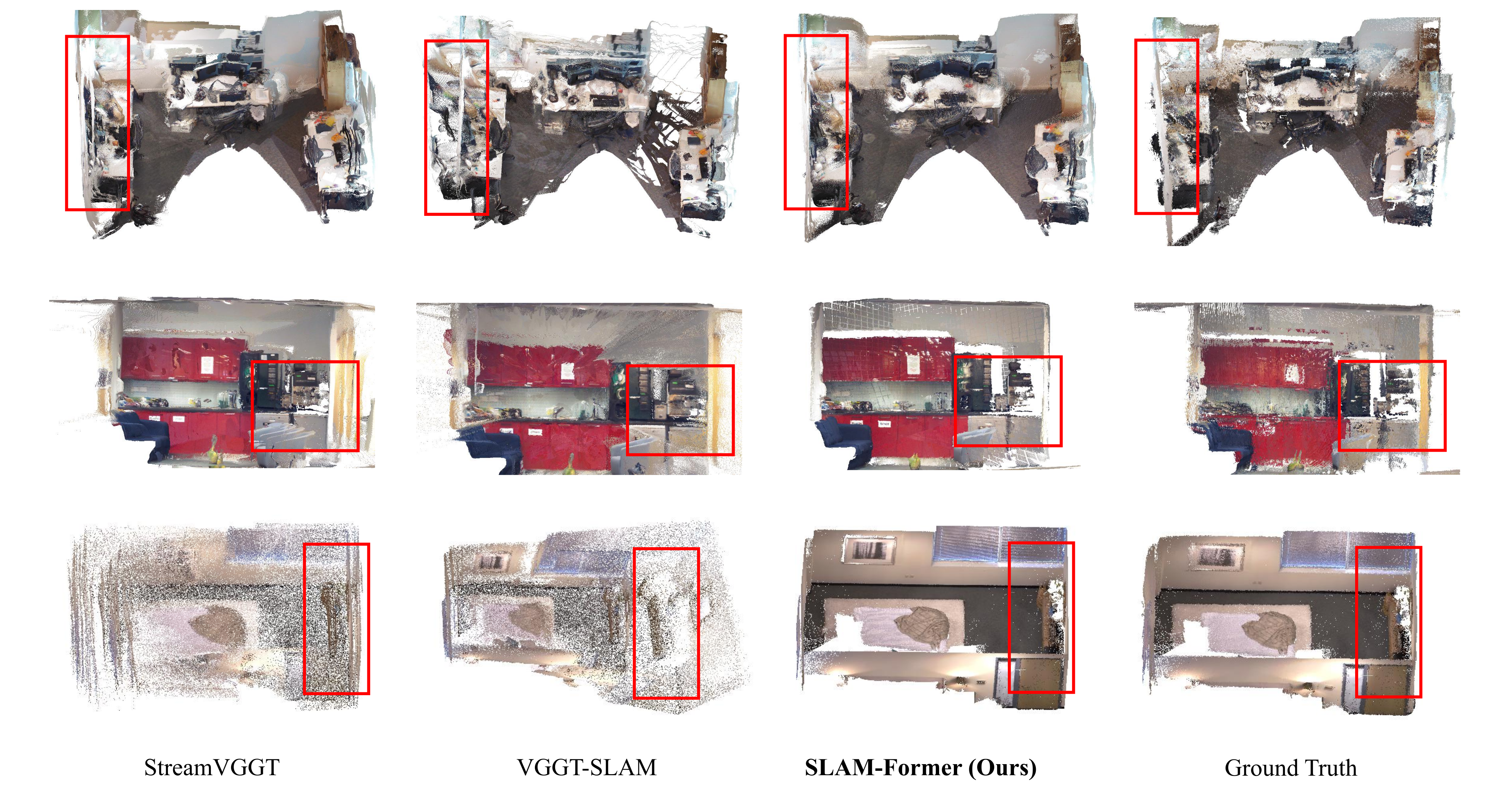
Figure 4 shows fewer duplicated or misaligned surfaces in selected office and pumpkin examples. These qualitative examples support structural consistency but do not replace the aggregate point-distance metrics.
Replica Reconstruction.
Replica’s reported average accuracy/completion is 2.09/1.56, compared with EC3R-SLAM’s 2.82/2.07 and MASt3R-SLAM’s 2.92/2.25. Table 5 does not label its units; these values should not be silently interpreted as the meter values used by Table 4. The average is best, but Room 0 favors EC3R-SLAM on both metrics.
Qualitative examples show fewer layered surfaces. Because evaluation samples a fixed number of points, apparent visual sparsity can reflect duplicated structures distributing those samples. The source refers to an additional MASt3R-SLAM comparison in Supplementary Figure C1, which is not included in this version’s 18-page PDF.
4.4 Frontend and backend co-operation
Table 6 reduces mean TUM trajectory error from 0.134 m with only the frontend to 0.039 m with the backend, a roughly 71% reduction. Every listed sequence improves, including room from 0.547 to 0.082 m. This is the most direct ablation supporting global refinement, though it combines backend correction and cache feedback rather than isolating each.
How does the backend assist the frontend?
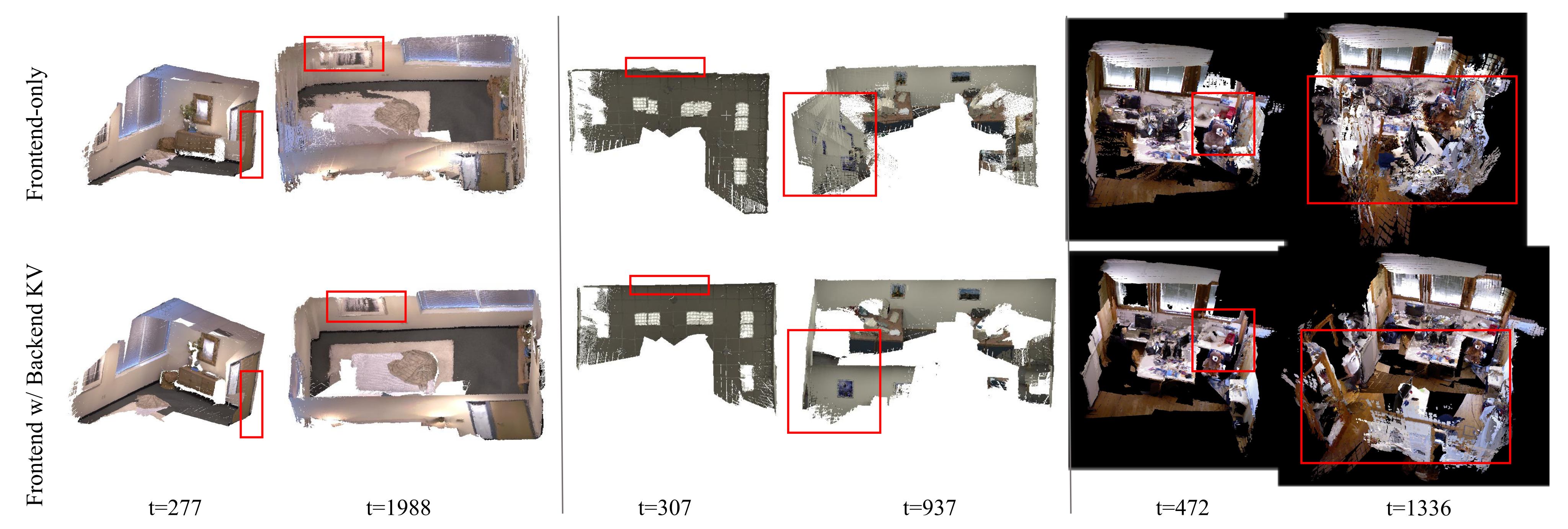
Figure 5 follows intermediate reconstructions of indoor loops. Frontend-only maps become increasingly distorted; backend-assisted maps remain more coherent in the selected examples. Cache replacement lets later observations use corrected history, providing a mechanism for reducing future drift as well as refining past output.
How does the backend benefit from the frontend?
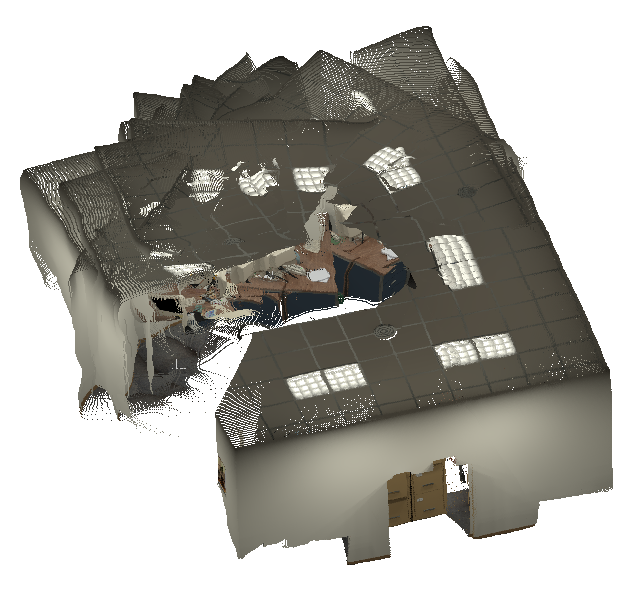
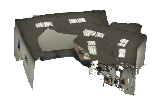
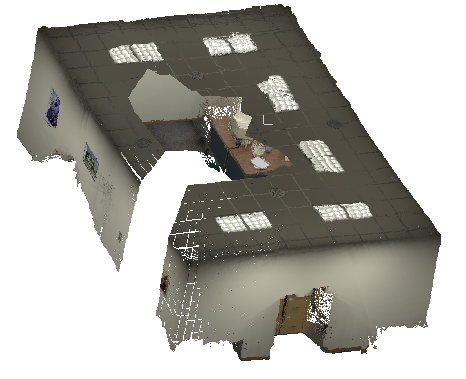
Figure 6 compares unordered-image VGGT/Pi3 reconstruction with SLAM-Former’s sequentially formed map tokens. The latter appears more coherent. This changes both the model and its processing history, so it does not isolate order information alone. The text names ICL-NUIM ofkt0, whereas the caption names ofkt1; that source inconsistency is retained rather than resolved by guessing.
4.5 Speeding up with KV Pruning
Table 7 keeps trajectory ATE at 0.042 m when retaining 12.5% of keys/values, but accuracy rises from 0.017 to 0.020 m and Chamfer from 0.026 to 0.029 m. These are about 18% and 12% increases, so “negligible” depends on the metric and application. At 6.25%, ATE grows to 0.055 m and accuracy to 0.026 m. Logarithmic and square-root cache schedules stay close to the full-cache scores.
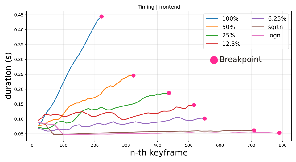
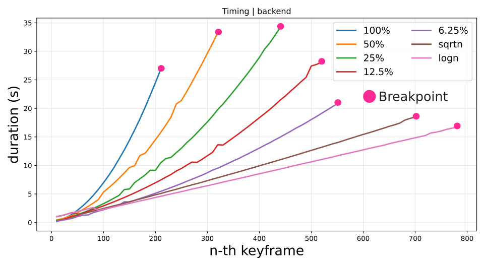
The full-cache Table 7 completeness/Chamfer values (0.036/0.026 m) differ slightly from Table 4’s 0.037/0.027 m. Figure 7 shows shorter frontend/backend runtimes and a later memory limit with pruning. Its endpoint is the memory breakpoint, not successful unlimited operation.
The plotted frontend can take tenths of a second at long histories, and backend passes can take many seconds. Thus the abstract’s real-time phrasing should be scoped to the incremental operation and tested history/settings, not read as a constant-latency guarantee for the entire growing map. Exact dynamic retention schedules and full end-to-end timing are not completely specified.
| Retained Ratio | 7-Scenes | |||
|---|---|---|---|---|
| ATE | Acc. | Complet. | Chamfer | |
| 100% | 0.042 | 0.017 | 0.036 | 0.026 |
| 50% | 0.041 | 0.017 | 0.036 | 0.027 |
| 25% | 0.042 | 0.018 | 0.037 | 0.027 |
| 12.5% | 0.042 | 0.020 | 0.038 | 0.029 |
| 6.25% | 0.055 | 0.026 | 0.042 | 0.034 |
| log KV pool | 0.042 | 0.017 | 0.037 | 0.027 |
| sqrt KV pool | 0.041 | 0.017 | 0.037 | 0.027 |
5 Conclusion
The main result is effective learned cooperation between a causal frontend and a globally revisiting backend, with shared weights and cache exchange. The benchmarks show particularly strong uncalibrated tracking and dense reconstruction, while calibrated geometric methods remain better in some settings.
Practical limits include increasing map/cache storage, periodic expensive global attention, sensitivity to learned priors and keyframe thresholds, and no explicit geometric guarantee. Dynamic scenes, prolonged tracking loss, outdoor deployment, uncertainty across training seeds and indefinite mapping are not established by these indoor benchmark results. A small-cache speedup should be weighed against metric-specific reconstruction degradation.
Acknowledgements
The work acknowledges support from the Beijing Municipal Science and Technology Program, grant Z251100008125011.