Literature
Display
← All papers

Compatibility of Multiple Control Barrier Functions for Constrained Nonlinear Systems

Max H. Cohen · Eugene Lavretsky · Aaron D. Ames

· IEEE Conference on Decision and Control (CDC 2025) ↗

Robotics4 min text · CondensedOriginal paper ↗
Contents

At a glance

Multiple safety constraints can conflict even when each is individually feasible. This paper identifies a structured case in which compatibility is guaranteed: independent outputs of a square nonlinear system, each restricted to an interval. Under a vector-relative-degree condition, paired exponential barriers yield a feasible, locally Lipschitz safety filter. A particular quadratic weight also gives a closed-form controller. Two planar-drone simulations illustrate the result.

I Introduction

A CBF turns forward invariance into an inequality on the control input. Combining several such inequalities raises three separate questions: whether any input satisfies them all, whether the selected controller is regular enough to define meaningful trajectories, and how filtering changes nominal tracking. This paper answers these questions for output box constraints, rather than arbitrary intersections of safe sets.

The construction uses the invertibility of the outputs’ decoupling matrix. It permits simultaneous constraints without requiring a separate online compatibility test. Its conclusions do not include actuator bounds: the control input is unconstrained apart from the barrier inequalities.

II Preliminaries

The analysis combines control barrier functions, relative-degree coordinates, and a feasibility condition for affine inequalities.

II-A Notation

The notation distinguishes Euclidean norms, matrix inequalities, and comparison functions. Local Lipschitz continuity is the regularity condition used for the feedback and its associated differential equation.

II-B Safety-Critical Control

For a control-affine system, a CBF defines a safe superlevel set and a linear inequality in the input. A quadratic program minimally changes a nominal command while enforcing that inequality. Standard invariance results require the barrier condition and a suitably regular feedback; a nonempty safe set alone does not establish either. [1]

Equations 1–10
𝐱˙=𝐟⁡(𝐱)+𝐠⁡(𝐱)​𝐮,\dot{\mathbf{x}}=\mathbf{f}(\mathbf{x})+\mathbf{g}(\mathbf{x})\mathbf{u}, (1)
𝒞≔{𝐱∈ℝn:h⁡(𝐱)≥0}.\mathcal{C}\coloneqq\{\mathbf{x}\in\mathbb{R}^{n}\,:\,h(\mathbf{x})\geq 0\}. (2)
𝐱˙=𝐟cl​(𝐱)≔𝐟⁡(𝐱)+𝐠⁡(𝐱)​𝐤​(𝐱).\dot{\mathbf{x}}=\mathbf{f}_{\rm{cl}}(\mathbf{x})\coloneqq\mathbf{f}(\mathbf{x})+\mathbf{g}(\mathbf{x})\mathbf{k}(\mathbf{x}). (3)
sup𝐮∈ℝm{L𝐟​h​(𝐱)+L𝐠​h​(𝐱)​𝐮}≥−α​h​(𝐱).\sup_{\mathbf{u}\in\mathbb{R}^{m}}\left\{L_{\mathbf{f}}h(\mathbf{x})+L_{\mathbf{g}}h(\mathbf{x})\mathbf{u}\right\}\geq-\alpha h(\mathbf{x}). (4)
L𝐠​h​(𝐱)=𝟎⟹L𝐟​h​(𝐱)+α​h​(𝐱)≥0,L_{\mathbf{g}}h(\mathbf{x})=\mathbf{0}\implies L_{\mathbf{f}}h(\mathbf{x})+\alpha h(\mathbf{x})\geq 0,
sr+αr​sr−1+⋯+α2​s+α1=∏i=1r(si−νi),s^{r}+\alpha_{r}s^{r-1}+\dots+\alpha_{2}s+\alpha_{1}=\prod_{i=1}^{r}(s_{i}-\nu_{i}), (5)
sup𝐮∈ℝm{L𝐟r​h​(𝐱)+L𝐠​L𝐟r−1​h​(𝐱)​𝐮}≥−𝜶⊤​𝐇​(𝐱),\sup_{\mathbf{u}\in\mathbb{R}^{m}}\left\{L_{\mathbf{f}}^{r}h(\mathbf{x})+L_{\mathbf{g}}L_{\mathbf{f}}^{r-1}h(\mathbf{x})\mathbf{u}\right\}\geq-\bm{\alpha}^{\top}\mathbf{H}(\mathbf{x}), (6)
ψ0​(𝐱)≔\displaystyle\psi_{0}(\mathbf{x})\coloneqq h⁡(𝐱)\displaystyle h(\mathbf{x}) (7)
ψi​(𝐱)≔\displaystyle\psi_{i}(\mathbf{x})\coloneqq dd​t​ψi−1​(𝐱)−νi​ψi−1​(𝐱),∀i∈{1,…,r},\displaystyle\frac{\mathrm{d}}{\mathrm{d}t}\psi_{i-1}(\mathbf{x})-\nu_{i}\psi_{i-1}(\mathbf{x}),\quad\forall i\in\{1,\dots,r\},
𝒞i={𝐱∈ℝn:ψi​(𝐱)≥0},∀i∈{0,…,r}.\mathcal{C}_{i}=\{\mathbf{x}\in\mathbb{R}^{n}\,:\,\psi_{i}(\mathbf{x})\geq 0\},\quad\forall i\in\{0,\dots,r\}. (8)
L𝐟r​h​(𝐱)+L𝐠​L𝐟r−1​h​(𝐱)​𝐤​(𝐱)≥−𝜶⊤​𝐇​(𝐱),L_{\mathbf{f}}^{r}h(\mathbf{x})+L_{\mathbf{g}}L_{\mathbf{f}}^{r-1}h(\mathbf{x})\mathbf{k}(\mathbf{x})\geq-\bm{\alpha}^{\top}\mathbf{H}(\mathbf{x}), (9)
𝐤⁡(𝐱)=arg​min𝐮∈ℝm\displaystyle\mathbf{k}(\mathbf{x})=\operatornamewithlimits{arg\,min}_{\mathbf{u}\in\mathbb{R}^{m}} 12​‖𝐮−𝐤d​(𝐱)‖𝐆⁡(𝐱)2\displaystyle\tfrac{1}{2}\|\mathbf{u}-\mathbf{k}_{\rm{d}}(\mathbf{x})\|_{\mathbf{G}(\mathbf{x})}^{2} (10)
s.t.\displaystyle\mathrm{s.t.} L𝐟r​h​(𝐱)+L𝐠​L𝐟r−1​h​(𝐱)​𝐮≥−𝜶⊤​𝐇​(𝐱)\displaystyle L_{\mathbf{f}}^{r}h(\mathbf{x})+L_{\mathbf{g}}L_{\mathbf{f}}^{r-1}h(\mathbf{x})\mathbf{u}\geq-\bm{\alpha}^{\top}\mathbf{H}(\mathbf{x})

II-C Outputs and Relative Degree

An output’s relative degree counts how many derivatives are needed before the input appears. For a square system with m inputs and m outputs, vector relative degree requires an invertible m-by-m decoupling matrix throughout the relevant domain. The derivative coordinates expose one input-dependent highest derivative for each output.

Equations 11
L𝐠​L𝐟j​yi​(𝐱)=0,L_{\mathbf{g}}L_{\mathbf{f}}^{j}y_{i}(\mathbf{x})=0,
𝐁⁡(𝐱)≔[L𝐠​L𝐟r1−1​y1​(𝐱)L𝐠​L𝐟rm−1​ym​(𝐱)]=[𝐛1​(𝐱)⊤𝐛m​(𝐱)⊤]∈ℝm×m,\mathbf{B}(\mathbf{x})\coloneqq\begin{bmatrix}L_{\mathbf{g}}L_{\mathbf{f}}^{r_{1}-1}y_{1}(\mathbf{x})\\ \vdots\\ L_{\mathbf{g}}L_{\mathbf{f}}^{r_{m}-1}y_{m}(\mathbf{x})\\ \end{bmatrix}=\begin{bmatrix}\mathbf{b}_{1}(\mathbf{x})^{\top}\\ \vdots\\ \mathbf{b}_{m}(\mathbf{x})^{\top}\\ \end{bmatrix}\in\mathbb{R}^{m\times m}, (11)

II-D Compatibility of Constraints

Compatibility means that all barrier inequalities have a common admissible input at each relevant state. Farkas’ lemma characterizes infeasibility through nonnegative multipliers. This algebraic alternative is the key tool for proving compatibility of the paired output constraints.

Equations 12–13
ci​(𝐱)+𝐝i​(𝐱)⊤​𝐮≥0,∀i∈ℐ.c_{i}(\mathbf{x})+\mathbf{d}_{i}(\mathbf{x})^{\top}\mathbf{u}\geq 0,\quad\forall i\in\mathcal{I}. (12)
∑i∈ℐλi​𝐝i​(𝐱)=𝟎⟹∑i∈ℐλi​ci​(𝐱)≥0.\sum_{i\in\mathcal{I}}\lambda_{i}\mathbf{d}_{i}(\mathbf{x})=\mathbf{0}\implies\sum_{i\in\mathcal{I}}\lambda_{i}c_{i}(\mathbf{x})\geq 0. (13)

III Compatibility of Multiple ECBFs

Each output has a strict lower and upper bound. An ECBF is built for each side using derivative coordinates and gains whose characteristic polynomial has real negative roots. The initial state must satisfy the resulting higher-order barrier conditions as well as the output bounds; starting inside the output box alone is insufficient for a high-relative-degree system.

The compatibility proof exploits independent rows of the decoupling matrix. In a potential Farkas certificate, the multipliers for an output’s lower and upper inequalities must match. The remaining expression is nonnegative because each interval has positive width, ruling out infeasibility. A lower and upper constraint for the same output cannot both be active. At most m independent constraints are active, which supports local Lipschitz continuity of the unique quadratic-program solution.

For the special cost matrix G = BᵀB, the optimization separates in the output-derivative coordinates. Theorem 3 gives explicit nonnegative multipliers and a closed-form correction, avoiding a numerical QP solve. This formula is not claimed for arbitrary positive-definite cost matrices. The preserved KKT equations and proof calculations specify the active-set cases.

Equations 14–27
[y¯1y¯m]⏟𝐲¯≤[y1​(𝐱)ym​(𝐱)]⏟𝐲⁡(𝐱)≤[y¯1y¯m]⏟𝐲¯,\underbrace{\begin{bmatrix}\underline{y}_{1}\\ \vdots\\ \underline{y}_{m}\end{bmatrix}}_{\underline{\mathbf{y}}}\leq\underbrace{\begin{bmatrix}y_{1}(\mathbf{x})\\ \vdots\\ y_{m}(\mathbf{x})\\ \end{bmatrix}}_{\mathbf{y}(\mathbf{x})}\leq\underbrace{\begin{bmatrix}\overline{y}_{1}\\ \vdots\\ \overline{y}_{m}\end{bmatrix}}_{\underline{\mathbf{y}}}, (14)
h¯i​(𝐱)=\displaystyle\underline{h}_{i}(\mathbf{x})= yi​(𝐱)−y¯i,\displaystyle y_{i}(\mathbf{x})-\underline{y}_{i}, (15)
h¯i​(𝐱)=\displaystyle\overline{h}_{i}(\mathbf{x})= y¯i−yi​(𝐱),\displaystyle\overline{y}_{i}-y_{i}(\mathbf{x}),
𝒞¯i≔\displaystyle\underline{\mathcal{C}}^{i}\coloneqq {𝐱∈ℝn:h¯i​(𝐱)≥0}={𝐱∈ℝn:yi​(𝐱)≥y¯i},\displaystyle\{\mathbf{x}\in\mathbb{R}^{n}\,:\,\underline{h}_{i}(\mathbf{x})\geq 0\}=\{\mathbf{x}\in\mathbb{R}^{n}\,:\,y_{i}(\mathbf{x})\geq\underline{y}_{i}\},
𝒞¯i≔\displaystyle\overline{\mathcal{C}}^{i}\coloneqq {𝐱∈ℝn:h¯i​(𝐱)≥0}={𝐱∈ℝn:yi​(𝐱)≤y¯i},\displaystyle\{\mathbf{x}\in\mathbb{R}^{n}\,:\,\overline{h}_{i}(\mathbf{x})\geq 0\}=\{\mathbf{x}\in\mathbb{R}^{n}\,:\,y_{i}(\mathbf{x})\leq\overline{y}_{i}\},
𝒞≔(⋂i=1m𝒞¯i)​⋂(⋂i=1m𝒞¯i).\mathcal{C}\coloneqq\left(\bigcap_{i=1}^{m}\underline{\mathcal{C}}^{i}\right)\bigcap\left(\bigcap_{i=1}^{m}\overline{\mathcal{C}}^{i}\right). (16)
𝒮≔(⋂i=1m𝒮¯i)​⋂(⋂i=1m𝒮¯i)⊂𝒞,\displaystyle\mathcal{S}\coloneqq\left(\bigcap_{i=1}^{m}\underline{\mathcal{S}}_{i}\right)\bigcap\left(\bigcap_{i=1}^{m}\overline{\mathcal{S}}_{i}\right)\subset\mathcal{C}, (17)
𝒮¯i≔⋂j=0ri𝒞¯ji𝒮¯i≔⋂j=0ri𝒞¯ji,\displaystyle\underline{\mathcal{S}}_{i}\coloneqq\bigcap_{j=0}^{r_{i}}\underline{\mathcal{C}}_{j}^{i}\quad\overline{\mathcal{S}}_{i}\coloneqq\bigcap_{j=0}^{r_{i}}\overline{\mathcal{C}}_{j}^{i}\quad,
min𝐮∈ℝm\displaystyle\min_{\mathbf{u}\in\mathbb{R}^{m}} 12​‖𝐮−𝐤d​(𝐱)‖𝐆⁡(𝐱)2\displaystyle\tfrac{1}{2}\|\mathbf{u}-\mathbf{k}_{\rm{d}}(\mathbf{x})\|_{\mathbf{G}(\mathbf{x})}^{2} (18)
s.t.\displaystyle\mathrm{s.t.} L𝐟ri​h¯i​(𝐱)+L𝐠​L𝐟ri−1​h¯i​(𝐱)​𝐮≥−𝜶i⊤​𝐇¯i​(𝐱)\displaystyle L_{\mathbf{f}}^{r_{i}}\underline{h}_{i}(\mathbf{x})+L_{\mathbf{g}}L_{\mathbf{f}}^{r_{i}-1}\underline{h}_{i}(\mathbf{x})\mathbf{u}\geq-{\bm{\alpha}}_{i}^{\top}\underline{\mathbf{H}}_{i}(\mathbf{x})
L𝐟ri​h¯i​(𝐱)+L𝐠​L𝐟ri−1​h¯i​(𝐱)​𝐮≥−𝜶i⊤​𝐇¯i​(𝐱)\displaystyle L_{\mathbf{f}}^{r_{i}}\overline{h}_{i}(\mathbf{x})+L_{\mathbf{g}}L_{\mathbf{f}}^{r_{i}-1}\overline{h}_{i}(\mathbf{x})\mathbf{u}\geq-{\bm{\alpha}}_{i}^{\top}\overline{\mathbf{H}}_{i}(\mathbf{x})
𝐇¯i​(𝐱)≔\displaystyle\underline{\mathbf{H}}_{i}(\mathbf{x})\coloneqq [h¯i​(𝐱)L𝐟​h¯i​(𝐱)…L𝐟ri−1​h¯i​(𝐱)]⊤\displaystyle\begin{bmatrix}\underline{h}_{i}(\mathbf{x})&L_{\mathbf{f}}\underline{h}_{i}(\mathbf{x})&\ldots&L_{\mathbf{f}}^{r_{i}-1}\underline{h}_{i}(\mathbf{x})\end{bmatrix}^{\top}
=\displaystyle= [yi​(𝐱)−y¯iL𝐟​yi​(𝐱)…L𝐟ri−1​yi​(𝐱)]⊤\displaystyle\begin{bmatrix}y_{i}(\mathbf{x})-\underline{y}_{i}&L_{\mathbf{f}}y_{i}(\mathbf{x})&\ldots&L_{\mathbf{f}}^{r_{i}-1}y_{i}(\mathbf{x})\end{bmatrix}^{\top}
𝐇¯i​(𝐱)≔\displaystyle\overline{\mathbf{H}}_{i}(\mathbf{x})\coloneqq [h¯i​(𝐱)L𝐟​h¯i​(𝐱)…L𝐟ri−1​h¯i​(𝐱)]⊤\displaystyle\begin{bmatrix}\overline{h}_{i}(\mathbf{x})&L_{\mathbf{f}}\overline{h}_{i}(\mathbf{x})&\ldots&L_{\mathbf{f}}^{r_{i}-1}\overline{h}_{i}(\mathbf{x})\end{bmatrix}^{\top}
=\displaystyle= [y¯i−yi​(𝐱)−L𝐟​yi​(𝐱)…−L𝐟ri−1​yi​(𝐱)]⊤.\displaystyle\begin{bmatrix}\overline{y}_{i}-y_{i}(\mathbf{x})&-L_{\mathbf{f}}y_{i}(\mathbf{x})&\ldots&-L_{\mathbf{f}}^{r_{i}-1}y_{i}(\mathbf{x})\end{bmatrix}^{\top}.
L𝐟ri​h¯i​(𝐱)=\displaystyle L_{\mathbf{f}}^{r_{i}}\underline{h}_{i}(\mathbf{x})= L𝐟r​yi​(𝐱)\displaystyle L_{\mathbf{f}}^{r}y_{i}(\mathbf{x}) (19)
L𝐟ri​h¯i​(𝐱)=\displaystyle L_{\mathbf{f}}^{r_{i}}\overline{h}_{i}(\mathbf{x})= −L𝐟r​yi​(𝐱)\displaystyle-L_{\mathbf{f}}^{r}y_{i}(\mathbf{x})
L𝐠​L𝐟ri−1​h¯i​(𝐱)=\displaystyle L_{\mathbf{g}}L_{\mathbf{f}}^{r_{i}-1}\underline{h}_{i}(\mathbf{x})= L𝐠​L𝐟ri−1​yi​(𝐱)\displaystyle L_{\mathbf{g}}L_{\mathbf{f}}^{r_{i}-1}y_{i}(\mathbf{x})
L𝐠​L𝐟ri−1​h¯i​(𝐱)=\displaystyle L_{\mathbf{g}}L_{\mathbf{f}}^{r_{i}-1}\overline{h}_{i}(\mathbf{x})= −L𝐠​L𝐟ri−1​yi​(𝐱),\displaystyle-L_{\mathbf{g}}L_{\mathbf{f}}^{r_{i}-1}y_{i}(\mathbf{x}),
min𝐮∈ℝm\displaystyle\min_{\mathbf{u}\in\mathbb{R}^{m}} 12​‖𝐮−𝐤d​(𝐱)‖𝐆⁡(𝐱)2\displaystyle\tfrac{1}{2}\|\mathbf{u}-\mathbf{k}_{\rm{d}}(\mathbf{x})\|_{\mathbf{G}(\mathbf{x})}^{2} (20)
s.t.\displaystyle\mathrm{s.t.} ai​(𝐱)+𝐛i​(𝐱)⊤​𝐮+α1i​(yi​(𝐱)−y¯i)≥0\displaystyle a_{i}(\mathbf{x})+\mathbf{b}_{i}(\mathbf{x})^{\top}\mathbf{u}+\alpha_{1}^{i}(y_{i}(\mathbf{x})-\underline{y}_{i})\geq 0
−ai​(𝐱)−𝐛i​(𝐱)⊤​𝐮−α1i​(yi​(𝐱)−y¯i)≥0,\displaystyle-a_{i}(\mathbf{x})-\mathbf{b}_{i}(\mathbf{x})^{\top}\mathbf{u}-\alpha_{1}^{i}(y_{i}(\mathbf{x})-\overline{y}_{i})\geq 0,
ai​(𝐱)≔\displaystyle a_{i}(\mathbf{x})\coloneqq L𝐟ri​yi​(𝐱)+∑j=1ri−1αj+1i​L𝐟j​yi​(𝐱).\displaystyle L_{\mathbf{f}}^{r_{i}}y_{i}(\mathbf{x})+\sum_{j=1}^{r_{i}-1}\alpha_{j+1}^{i}L_{\mathbf{f}}^{j}y_{i}(\mathbf{x}). (21)
cj​(𝐱)≔\displaystyle c_{j}(\mathbf{x})\coloneqq aj​(𝐱)+α1j​(yj​(𝐱)−y¯j)\displaystyle a_{j}(\mathbf{x})+\alpha_{1}^{j}(y_{j}(\mathbf{x})-\underline{y}_{j}) (22)
cj+1​(𝐱)≔\displaystyle c_{j+1}(\mathbf{x})\coloneqq −aj​(𝐱)−α1j​(yj​(𝐱)−y¯j)\displaystyle-a_{j}(\mathbf{x})-\alpha_{1}^{j}(y_{j}(\mathbf{x})-\overline{y}_{j})
𝐝j​(𝐱)=\displaystyle\mathbf{d}_{j}(\mathbf{x})= 𝐛j​(𝐱)\displaystyle\mathbf{b}_{j}(\mathbf{x})
𝐝j+1​(𝐱)=\displaystyle\mathbf{d}_{j+1}(\mathbf{x})= −𝐛j​(𝐱),\displaystyle-\mathbf{b}_{j}(\mathbf{x}),
∑j=12​mλj​𝐝j​(𝐱)=∑i=1m(λ¯i−λ¯i)​𝐛i​(𝐱)=∑i=1pμi​𝐛i​(𝐱),\displaystyle\sum_{j=1}^{2m}\lambda_{j}\mathbf{d}_{j}(\mathbf{x})=\sum_{i=1}^{m}(\underline{\lambda}_{i}-\overline{\lambda}_{i})\mathbf{b}_{i}(\mathbf{x})=\sum_{i=1}^{p}\mu_{i}\mathbf{b}_{i}(\mathbf{x}),
∑i=1mμi​𝐛i​(𝐱)=𝟎⇔\displaystyle\sum_{i=1}^{m}\mu_{i}\mathbf{b}_{i}(\mathbf{x})=\mathbf{0}\iff μi=0,∀i∈{1,…,m}\displaystyle\mu_{i}=0,\;\forall i\in\{1,\dots,m\} (23)
⇔\displaystyle\iff λ¯i=λ¯i,∀i∈{1,…,m}.\displaystyle\underline{\lambda}_{i}=\overline{\lambda}_{i},\;\forall i\in\{1,\dots,m\}.
∑j=12​mλj​cj​(𝐱)=\displaystyle\sum_{j=1}^{2m}\lambda_{j}c_{j}(\mathbf{x})= ∑i=1mλ¯i​[ai​(𝐱)+α1i​(yi​(𝐱)−y¯i)]\displaystyle\sum_{i=1}^{m}\underline{\lambda}_{i}\left[a_{i}(\mathbf{x})+\alpha_{1}^{i}(y_{i}(\mathbf{x})-\underline{y}_{i})\right]
−∑i=1mλ¯i[ai(𝐱)+α1j(yi(𝐱)−y¯i)]\displaystyle-\sum_{i=1}^{m}\overline{\lambda}_{i}\left[a_{i}(\mathbf{x})+\alpha_{1}^{j}(y_{i}(\mathbf{x})-\overline{y}_{i})\right]
=\displaystyle= ∑i=1mλ¯i​α1i​[y¯i−y¯i]≥0,\displaystyle\sum_{i=1}^{m}\underline{\lambda}_{i}\alpha_{1}^{i}\left[\overline{y}_{i}-\underline{y}_{i}\right]\geq 0,
cj​(𝐱)+𝐝j​(𝐱)​𝐮∗​(𝐱)=0,c_{j}(\mathbf{x})+\mathbf{d}_{j}(\mathbf{x})\mathbf{u}^{*}(\mathbf{x})=0, (24)
ai​(𝐱)+𝐛i​(𝐱)⊤​𝐮∗​(𝐱)+α1i​(yi​(𝐱)−y¯i)=\displaystyle a_{i}(\mathbf{x})+\mathbf{b}_{i}(\mathbf{x})^{\top}\mathbf{u}^{*}(\mathbf{x})+\alpha_{1}^{i}(y_{i}(\mathbf{x})-\underline{y}_{i})= 0\displaystyle 0
−ai​(𝐱)−𝐛i​(𝐱)⊤​𝐮∗​(𝐱)−α1i​(yi​(𝐱)−y¯i)=\displaystyle-a_{i}(\mathbf{x})-\mathbf{b}_{i}(\mathbf{x})^{\top}\mathbf{u}^{*}(\mathbf{x})-\alpha_{1}^{i}(y_{i}(\mathbf{x})-\overline{y}_{i})= 0.\displaystyle 0.
[cj1​(𝐱)cj|𝒜⁡(𝐱)|​(𝐱)]⏟𝐜⁡(𝐱)+[𝐝j1​(𝐱)⊤𝐝j|𝒜⁡(𝐱)|​(𝐱)⊤]⏟𝐃⁡(𝐱)=𝟎,\underbrace{\begin{bmatrix}c_{j_{1}}(\mathbf{x})\\ \vdots\\ c_{j_{|\mathcal{A}(\mathbf{x})|}}(\mathbf{x})\end{bmatrix}}_{\mathbf{c}(\mathbf{x})}+\underbrace{\begin{bmatrix}\mathbf{d}_{j_{1}}(\mathbf{x})^{\top}\\ \vdots\\ \mathbf{d}_{j_{|\mathcal{A}(\mathbf{x})|}}(\mathbf{x})^{\top}\end{bmatrix}}_{\mathbf{D}(\mathbf{x})}=\mathbf{0},
𝐲¯≤𝐲⁡(𝐱⁡(t))≤𝐲¯,∀t≥0.\underline{\mathbf{y}}\leq\mathbf{y}(\mathbf{x}(t))\leq\overline{\mathbf{y}},\quad\forall t\geq 0. (25)
L𝐟ri​h¯i​(𝐱)+L𝐠​L𝐟ri−1​h¯i​(𝐱)​𝐤​(𝐱)≥−𝜶i⊤​𝐇¯i​(𝐱),\displaystyle L_{\mathbf{f}}^{r_{i}}\underline{h}_{i}(\mathbf{x})+L_{\mathbf{g}}L_{\mathbf{f}}^{r_{i}-1}\underline{h}_{i}(\mathbf{x})\mathbf{k}(\mathbf{x})\geq-{\bm{\alpha}}_{i}^{\top}\underline{\mathbf{H}}_{i}(\mathbf{x}), (26)
L𝐟ri​h¯i​(𝐱)+L𝐠​L𝐟ri−1​h¯i​(𝐱)​𝐤​(𝐱)≥−𝜶i⊤​𝐇¯i​(𝐱),\displaystyle L_{\mathbf{f}}^{r_{i}}\overline{h}_{i}(\mathbf{x})+L_{\mathbf{g}}L_{\mathbf{f}}^{r_{i}-1}\overline{h}_{i}(\mathbf{x})\mathbf{k}(\mathbf{x})\geq-{\bm{\alpha}}_{i}^{\top}\overline{\mathbf{H}}_{i}(\mathbf{x}),
𝐮∗​(𝐱)=\displaystyle\mathbf{u}^{*}(\mathbf{x})= 𝐤d​(𝐱)+∑i=1m(λ¯i∗​(𝐱)−λ¯i∗​(𝐱))​𝐆−1​(𝐱)​𝐛i​(𝐱),\displaystyle\mathbf{k}_{\rm{d}}(\mathbf{x})+\sum_{i=1}^{m}\big(\underline{\lambda}^{*}_{i}(\mathbf{x})-\overline{\lambda}^{*}_{i}(\mathbf{x})\big)\mathbf{G}^{-1}(\mathbf{x})\mathbf{b}_{i}(\mathbf{x}), (27)
λ¯i∗​(𝐱)=\displaystyle\underline{\lambda}^{*}_{i}(\mathbf{x})= max⁡{0,−ω¯i​(𝐱)},\displaystyle\max\{0,-\underline{\omega}_{i}(\mathbf{x})\},
λ¯i∗​(𝐱)=\displaystyle\overline{\lambda}^{*}_{i}(\mathbf{x})= max⁡{0,−ω¯i​(𝐱)},\displaystyle\max\{0,-\overline{\omega}_{i}(\mathbf{x})\},
ω¯i​(𝐱)≔\displaystyle\underline{\omega}_{i}(\mathbf{x})\coloneqq ai​(𝐱)+α1i​(yi​(𝐱)−y¯i)+𝐛i​(𝐱)⊤​𝐤d​(𝐱),\displaystyle a_{i}(\mathbf{x})+\alpha_{1}^{i}(y_{i}(\mathbf{x})-\underline{y}_{i})+\mathbf{b}_{i}(\mathbf{x})^{\top}\mathbf{k}_{\rm{d}}(\mathbf{x}),
ω¯i​(𝐱)≔\displaystyle\overline{\omega}_{i}(\mathbf{x})\coloneqq −ai​(𝐱)−α1i​(yi​(𝐱)−y¯i)−𝐛i​(𝐱)⊤​𝐤d​(𝐱),\displaystyle-a_{i}(\mathbf{x})-\alpha_{1}^{i}(y_{i}(\mathbf{x})-\overline{y}_{i})-\mathbf{b}_{i}(\mathbf{x})^{\top}\mathbf{k}_{\rm{d}}(\mathbf{x}),
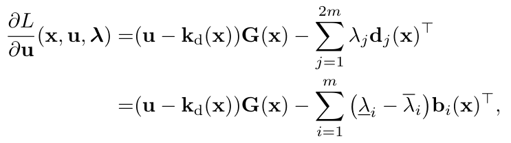
Lagrangian (28)
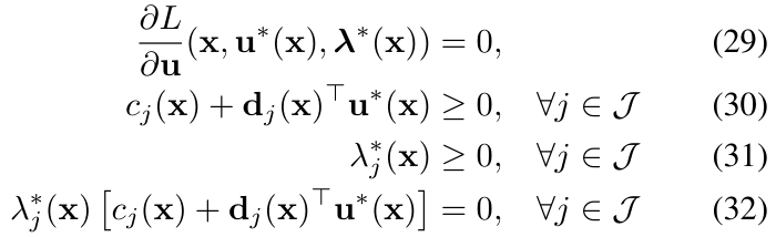
Karush–Kuhn–Tucker conditions (29–32)
Stationarity substitution
Primal feasibility inequalities
Weighted Gram identity
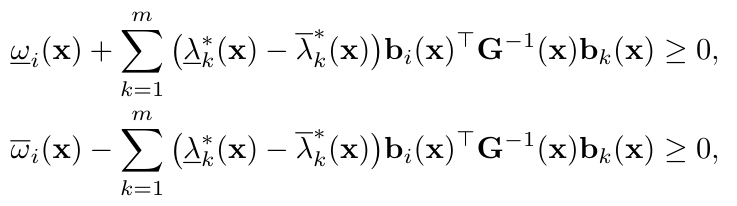
Feasibility reduction (33)
Definition of the inequality left-hand side
Cases i–iii
Contradiction for case iv
Complementary slackness

IV Stability Analysis

The safe output interval gives a bound on tracking error when the desired output is bounded. A stronger result treats the safety-filter correction as an input to a nominally stable tracking system. Under the stated Lyapunov, compactness, regularity, and reference assumptions, the error obeys an ISS bound determined by the intervention magnitude.

This quantifies degradation of nominal performance; it does not promise exact tracking of an unsafe reference. Safety and tracking remain distinct objectives, and bounded output coordinates alone need not bound every internal state.

Equations 34–43
𝐞⁡(𝐱,t)≔𝐲⁡(𝐱)−𝐲d​(t),\mathbf{e}(\mathbf{x},t)\coloneqq\mathbf{y}(\mathbf{x})-\mathbf{y}_{\rm{d}}(t), (34)
ρ​‖𝐞⁡(𝐱,t)‖2≤V⁡(𝐱,t),\rho\|\mathbf{e}(\mathbf{x},t)\|^{2}\leq V(\mathbf{x},t), (35)
∂V∂t​(𝐱,t)+∂V∂𝐱​(𝐱,t)​[𝐟⁡(𝐱)+𝐠⁡(𝐱)​𝐤d​(𝐱,t)]\displaystyle\frac{\partial V}{\partial t}(\mathbf{x},t)+\frac{\partial V}{\partial\mathbf{x}}(\mathbf{x},t)\big[\mathbf{f}(\mathbf{x})+\mathbf{g}(\mathbf{x})\mathbf{k}_{\rm{d}}(\mathbf{x},t)\big] (36)
≤−γ​V​(𝐱,t)−σ​‖∂V∂𝐱​(𝐱,t)​𝐠​(𝐱)‖2,\displaystyle\leq-\gamma V(\mathbf{x},t)-\sigma\left\|\frac{\partial V}{\partial\mathbf{x}}(\mathbf{x},t)\mathbf{g}(\mathbf{x})\right\|^{2},
‖𝐞⁡(𝐱⁡(t),t)‖≤β⁡(V⁡(𝐱⁡(0),0),t)+ι⁡(‖𝐤cbf​(𝐱⁡(t),t)‖∞),\|\mathbf{e}(\mathbf{x}(t),t)\|\leq\beta(V(\mathbf{x}(0),0),t)+\iota(\|\mathbf{k}_{\rm{cbf}}(\mathbf{x}(t),t)\|_{\infty}), (37)
𝐤cbf​(𝐱,t)≔∑i=1m(λ¯i​(𝐱,t)−λ¯i​(𝐱,t))​𝐆−1​(𝐱)​𝐛i​(𝐱),\mathbf{k}_{\rm{cbf}}(\mathbf{x},t)\coloneqq\sum_{i=1}^{m}(\underline{\lambda}_{i}(\mathbf{x},t)-\overline{\lambda}_{i}(\mathbf{x},t))\mathbf{G}^{-1}(\mathbf{x})\mathbf{b}_{i}(\mathbf{x}), (38)
V˙​(𝐱,t)=\displaystyle\dot{V}(\mathbf{x},t)= ∂V∂t​(𝐱,t)+∂V∂𝐱​(𝐱,t)​[𝐟⁡(𝐱)+𝐠⁡(𝐱)​𝐤d​(𝐱,t)]\displaystyle\frac{\partial V}{\partial t}(\mathbf{x},t)+\frac{\partial V}{\partial\mathbf{x}}(\mathbf{x},t)\big[\mathbf{f}(\mathbf{x})+\mathbf{g}(\mathbf{x})\mathbf{k}_{\rm{d}}(\mathbf{x},t)\big]
+∂V∂𝐱​(𝐱,t)​𝐠​(𝐱)​𝐤cbf​(𝐱,t).\displaystyle+\frac{\partial V}{\partial\mathbf{x}}(\mathbf{x},t)\mathbf{g}(\mathbf{x})\mathbf{k}_{\rm{cbf}}(\mathbf{x},t).
V˙​(𝐱,t)≤\displaystyle\dot{V}(\mathbf{x},t)\leq −γ​V​(𝐱,t)−σ​‖∂V∂𝐱​(𝐱,t)​𝐠​(𝐱)‖2\displaystyle-\gamma V(\mathbf{x},t)-\sigma\left\|\frac{\partial V}{\partial\mathbf{x}}(\mathbf{x},t)\mathbf{g}(\mathbf{x})\right\|^{2} (39)
+‖∂V∂𝐱​(𝐱,t)​𝐠​(𝐱)​𝐤cbf​(𝐱,t)‖,\displaystyle+\left\|\frac{\partial V}{\partial\mathbf{x}}(\mathbf{x},t)\mathbf{g}(\mathbf{x})\mathbf{k}_{\rm{cbf}}(\mathbf{x},t)\right\|,
V˙​(𝐱,t)≤\displaystyle\dot{V}(\mathbf{x},t)\leq −γ​V​(𝐱,t)−σ​‖∂V∂𝐱​(𝐱,t)​𝐠​(𝐱)‖2\displaystyle-\gamma V(\mathbf{x},t)-\sigma\left\|\frac{\partial V}{\partial\mathbf{x}}(\mathbf{x},t)\mathbf{g}(\mathbf{x})\right\|^{2} (40)
+‖∂V∂𝐱(𝐱,t)𝐠(𝐱)‖⋅∥𝐤cbf(𝐱,t)∥.\displaystyle+\left\|\frac{\partial V}{\partial\mathbf{x}}(\mathbf{x},t)\mathbf{g}(\mathbf{x})\right\|\cdot\|\mathbf{k}_{\rm{cbf}}(\mathbf{x},t)\|.
V˙​(𝐱,t)≤−γ​V​(𝐱,t)+‖𝐤cbf​(𝐱,t)‖24​σ.\dot{V}(\mathbf{x},t)\leq-\gamma V(\mathbf{x},t)+\frac{\|\mathbf{k}_{\rm{cbf}}(\mathbf{x},t)\|^{2}}{4\sigma}. (41)
V˙​(𝐱,t)≤−γ​V​(𝐱,t)+‖𝐤cbf​(𝐱⁡(t),t)‖∞24​σ.\displaystyle\dot{V}(\mathbf{x},t)\leq-\gamma V(\mathbf{x},t)+\frac{\|\mathbf{k}_{\rm{cbf}}(\mathbf{x}(t),t)\|_{\infty}^{2}}{4\sigma}. (42)
V⁡(𝐱⁡(t),t)≤V⁡(𝐱⁡(0),0)​e−γ​t+‖𝐤cbf​(𝐱⁡(t),t)‖∞24​γ​σ,V(\mathbf{x}(t),t)\leq V(\mathbf{x}(0),0)e^{-\gamma t}+\frac{\|\mathbf{k}_{\rm{cbf}}(\mathbf{x}(t),t)\|_{\infty}^{2}}{4\gamma\sigma}, (43)

V Numerical Examples

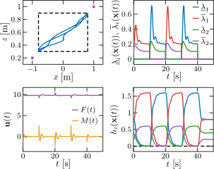
Both examples use a simulated planar quadrotor. They demonstrate the structured compatibility result and how the filter changes commands near several active boundaries.

V-A Planar Drone

The full six-state drone uses thrust and moment to constrain height and attitude. The selected outputs have relative degree two, with a decoupling matrix that is nonsingular when the attitude stays strictly between −π/2 and π/2. The barrier gains are (1, 2), and the quadratic weight is BᵀB.

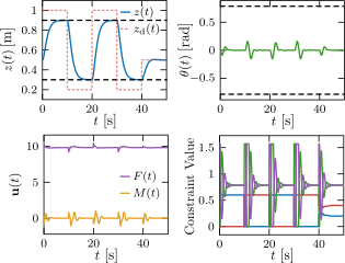
The nominal position controller requests setpoints outside the allowed output range. The safety filter keeps the constrained outputs within bounds while sacrificing the incompatible tracking objective. Figure 1 includes the resulting trajectories and barrier behavior; this is simulation evidence, without additional actuator-limit guarantees.

Equations 44
𝐟⁡(𝐱)=[x˙z˙θ˙0−g0],𝐠⁡(𝐱)=[000000−sin⁡(θ)0cos⁡(θ)001],\mathbf{f}(\mathbf{x})=\begin{bmatrix}\dot{x}\\ \dot{z}\\ \dot{\theta}\\ 0\\ -g\\ 0\end{bmatrix},\quad\mathbf{g}(\mathbf{x})=\begin{bmatrix}0&0\\ 0&0\\ 0&0\\ -\sin(\theta)&0\\ \cos(\theta)&0\\ 0&1\end{bmatrix}, (44)
𝐁⁡(𝐱)=[cos⁡(θ)001],\mathbf{B}(\mathbf{x})=\begin{bmatrix}\cos(\theta)&0\\ 0&1\end{bmatrix},
𝒞={𝐱∈ℝn:zmin≤z≤zmax,θmin≤θ≤θmax},\mathcal{C}=\{\mathbf{x}\in\mathbb{R}^{n}\,:\,z_{\min}\leq z\leq z_{\max},\,\theta_{\min}\leq\theta\leq\theta_{\max}\},
Original figure
Figure 1: Closed-loop trajectories of the drone example from Sec. V-A showing the drone’s vertical position (top left), orientation (top right), inputs (bottom left), and ECBF constraints (bottom right).

V-B More Complex Constraints via Reduced-Order Models

A reduced double-integrator model constrains horizontal and vertical position to a rectangle. Several boundaries can become active together at a corner. The filter maintains the model’s constraints and redirects unsafe reference tracking.

Applying this reduced-order command to the physical drone relies on a sufficiently accurate tracking controller and the assumptions of the cited reduced-order safety framework. [29], [30] The example does not establish unconditional safety of arbitrary full-order tracking dynamics.

Equations 45–46
𝐳˙=[x˙z˙0−g]+[00001001]​𝐯,\dot{\mathbf{z}}=\begin{bmatrix}\dot{x}\\ \dot{z}\\ 0\\ -g\end{bmatrix}+\begin{bmatrix}0&0\\ 0&0\\ 1&0\\ 0&1\end{bmatrix}\mathbf{v}, (45)
𝐳(t)∈𝒞={𝐳∈ℝ4:xmin≤x≤xmax,zmin≤z≤zmax}\mathbf{z}(t)\in\mathcal{C}=\{\mathbf{z}\in\mathbb{R}^{4}\,:\,x_{\min}\leq x\leq x_{\max},z_{\min}\leq z\leq z_{\max}\}
F=\displaystyle F= [−sin⁡(θ)cos⁡(θ)]†​𝐤𝐳​(x,z,x˙,z˙),\displaystyle\begin{bmatrix}-\sin(\theta)\\ \cos(\theta)\end{bmatrix}^{\dagger}\mathbf{k}_{\mathbf{z}}(x,z,\dot{x},\dot{z}), (46)
θd=\displaystyle\theta_{\rm{d}}= atan2⁡(𝐤𝐳,1​(x,z,x˙,z˙),𝐤𝐳,2​(x,z,x˙,z˙)),\displaystyle\operatorname{atan2}\left(\mathbf{k}_{\mathbf{z},1}(x,z,\dot{x},\dot{z}),\mathbf{k}_{\mathbf{z},2}(x,z,\dot{x},\dot{z})\right),
Original figure
Figure 2: Closed-loop trajectories of the drone example from Sec. V-B showing the drone’s (x,z)(x,z) position (top left), the Lagrange multipliers associated with the closed-form QP controller from (27) (top right), the control inputs (bottom left), and the ECBFs (bottom right).

VI Conclusions

Output box constraints with a nonsingular vector-relative-degree structure admit mutually compatible ECBFs, a regular safety filter, and, with a matched cost, an explicit solution. The practical scope is limited by that structure, the required initial higher-order conditions, and unrestricted control authority. Future work includes more general constraints and extensions beyond the present assumptions.

Acknowledgments

The authors thank Heather Hussain for discussions.

Concept demonstration

Open image ↗